1. Introduction
Anomaly detection on complex networks underpins applications in communication security, finance, and cyber-physical systems. Recent progress in graph representation learning has produced powerful detectors, yet most methods emphasize empirical accuracy while offering limited certification of reliability under sampling constraints [
1,
2]. This gap is acute in high-throughput settings where full-graph access is costly and decision risk must be controlled.
In our earlier work on scalable intrusion detection via property testing and federated edge AI [
3] and on property-based testing for cybersecurity [
4], we demonstrated how lightweight testing and distributed learning can enhance anomaly detection in resource-constrained settings. However, those approaches primarily established empirical effectiveness and automation benefits, without providing a formal certificate on the probability of missed anomalies. The present study advances this line of research by introducing a tester-guided graph learner that incorporates provable sampling guarantees, moving from heuristic detection toward verifiable reliability.
Beyond methodological novelty, the ability to report certified detection risk has direct impact in practice. In domains such as financial fraud, network security, and critical infrastructure monitoring, stakeholders require not only accurate predictions but also quantifiable guarantees under bounded sampling budgets. Traditional empirical detectors cannot offer such assurances, leaving decision-makers to rely on heuristic thresholds. By contrast, our certificate provides an explicit, finite-sample upper bound on missed detections, enabling risk-aware deployment in high-stakes settings.
We address this need with a tester-guided learner, PT-GNN, that couples sublinear graph property testing with lightweight learning to obtain an
end-to-end miss-probability certificate. Property testing offers principled, query-efficient procedures to assess global graph structure from local probes [
5,
6], and triangle-based motifs (closure/cluster structure) are canonical indicators for community coherence and irregular interaction patterns. We instantiate the tester via wedge sampling for triangle statistics, a technique with provable accuracy guarantees and practical efficiency on large graphs [
7,
8].
Unlike existing anomaly detection methods that either rely solely on empirical accuracy (e.g., GNN-based detectors) or offer generic certified guarantees without graph-specific considerations (e.g., randomized smoothing, conformal prediction), our approach uniquely integrates property testing with graph learning. Specifically, PT-GNN is the first framework to couple wedge-sampling with lightweight graph classification in order to produce an end-to-end miss-probability certificate . This moves beyond heuristic scoring or robustness guarantees by providing task-specific, finite-sample reliability bounds directly tied to triangle-based anomalies. Triangles are a canonical indicator of collusion and dense substructures—patterns observed in fraud rings, insider trading, and coordinated botnets. By targeting anomalies characterized by abnormal closure frequency, PT-GNN bridges a critical gap: it provides both strong empirical detection and formally verifiable guarantees under sampling constraints, ensuring that decisions can be deployed with quantifiable risk.
Our certificate decomposes the probability of missing an anomaly into two additive terms:
a tester uncertainty term
obtained from a Bernstein-type concentration bound on the wedge-sampling estimator, and
a classifier validation error
from supervised evaluation. The overall miss-probability is thus upper-bounded by
, directly linking sampling budget to decision risk via nonasymptotic concentration results [
9].
Our contributions are as follows:
We introduce PT-GNN, a tester-guided graph learner that integrates wedge-sampling triangle closure into training and reporting.
We derive an end-to-end miss-probability certificate that combines a Bernstein-style bound for the tester with empirical validation error for the learner.
On synthetic communication-graph benchmarks, we show perfect detection (AUC/F1) alongside systematically tightening certificates as the tester budget increases, demonstrating practical verifiability under bounded sampling.
We extend our prior work [
3,
4] by providing, for the first time, formally certified detection guarantees in addition to strong empirical performance.
2. Related Work
Research on anomaly detection in graphs intersects multiple lines of investigation. We briefly review relevant contributions on motif-based detection, sublinear property testing, graph representation learning, and certified machine learning.
Recent surveys highlight the diversity of approaches to graph anomaly detection. Song [
10] provides a concise 2024 overview, while Pazho et al. [
11] and Ekle & Eberle [
12] review deep graph anomaly detection and dynamic-graph methods, respectively. These works frame the broader landscape to which PT-GNN contributes.
2.1. Motif-Based Anomaly Detection
Network motifs such as wedges and triangles are central in characterizing community structure and irregularities. Early work showed that deviations in triangle closure often signal spurious or anomalous links [
13]. Methods exploiting subgraph patterns and clustering coefficients have been applied in social and communication networks [
1,
14]. Efficient wedge-sampling estimators enable scalable motif statistics on large graphs [
7,
8]. Our work adopts wedge-based testing as a backbone, but departs from heuristic anomaly scores by coupling motif statistics with an explicit concentration bound that contributes to a miss-probability certificate.
Complementary efforts include Ai et al. [
15], who study group-level anomalies via topology patterns, broadening anomaly definitions beyond wedges and triangles.
2.2. Sublinear Graph Property Testing
Graph property testing provides query-efficient algorithms to approximate global properties from local samples [
5,
6]. Applications range from connectivity and bipartiteness testing to motif frequency estimation. Concentration inequalities have been leveraged to provide probabilistic guarantees on tester outputs [
9]. In security, property testing has been recently explored for protocol validation and intrusion detection in distributed settings [
3,
4]. PT-GNN extends these ideas by embedding a tester directly into a learning pipeline, enabling certificates that span both sampling and classification.
2.3. Graph Representation Learning for Anomalies
Graph neural networks (GNNs) and representation models have been widely studied for anomaly detection [
2]. Approaches range from autoencoder-based detection [
16] to community-preserving embeddings and spectral methods. While effective, most methods remain empirical and do not quantify detection risk. Prior work on federated and edge-based anomaly detection [
3] highlights the need for lightweight and distributed solutions, yet still lacks verifiable guarantees. PT-GNN contributes to this line by combining efficient motif-level queries with certifiable bounds, offering both scalability and formal reliability.
Recent methods continue to diversify. Roy et al. [
17] reconstruct local neighborhoods for anomaly scores, while Tian et al. [
18] introduce semi-supervised detection on dynamic graphs. Yang et al. [
19] propose GRAM, an interpretable gradient-attention approach that emphasizes model transparency in anomaly detection.
2.4. Certified Learning and Detection Guarantees
Certified machine learning has recently sought to quantify model reliability beyond empirical metrics. Randomized smoothing offers provable robustness against adversarial perturbations [
20], while conformal prediction provides finite-sample confidence sets [
21]. In anomaly detection, guarantees remain scarce, with most work focusing on distribution-free confidence intervals or heuristic thresholds. By introducing a
certificate that combines tester variance with validation error, PT-GNN situates itself within this emerging paradigm of verifiable detection.
Knowledge-enabled frameworks such as KnowGraph [
22] further show how domain knowledge can be integrated with graph anomaly detection, offering an orthogonal perspective to certified reliability.
To summarize the positioning of our approach relative to prior work,
Table 1 contrasts motif-based, property-testing, GNN-based, and certified ML methods. As the table highlights, while existing approaches offer either scalability or strong empirical performance, none provide end-to-end formal guarantees for anomaly detection in complex networks. PT-GNN uniquely integrates sublinear property testing with representation learning to deliver both scalability and certified reliability.
Taken together, these comparisons highlight the position of PT-GNN relative to the field. Unlike motif-based anomaly detectors, PT-GNN moves beyond heuristic subgraph statistics by embedding a wedge-based tester into a certified learning pipeline. Compared with property-testing approaches, it extends guarantees from the tester alone to the entire end-to-end detection process. Relative to GNN-based methods, it preserves scalability while offering formal reliability that empirical models cannot provide. Finally, in contrast to certified ML frameworks such as randomized smoothing or conformal prediction, PT-GNN is graph-specific and tailored to triangle-driven irregularities. At the same time, we acknowledge that PT-GNN shares certain limitations with these families, such as sensitivity to anomaly definitions and dependence on validation data for calibration. This synthesis underscores the contribution of PT-GNN: it is, to our knowledge, the first approach to provide scalable, triangle-specific, and formally certified anomaly detection in complex networks.
3. Method
We detail PT-GNN’s components and the derivation of the end-to-end miss-probability certificate -from the problem formulation to the wedge tester, classifier, and computational cost.
3.1. Problem Setting
Let
be a simple undirected graph and let a
wedge be an unordered length-2 path
with edges
. A wedge is
closed if
, otherwise it is
open. For a graph
G, define the
triangle-closure probability as follows:
Intuitively,
quantifies the tendency of the network to form closed triads. In many real-world settings, unusually high closure rates can reveal coordinated or collusive behavior. For example, fraud rings and insider-trading groups often create tightly interconnected communities, while botnet controllers may generate bursts of dense triadic communication. Conversely, benign background traffic or random interactions tend to produce wedges that remain open. Thus, differences in
between normal and anomalous graphs capture structural irregularities that are difficult to detect from degree information alone.
We consider i.i.d. labeled samples , with indicating an anomaly class characterized by overexpressed triangle closure. Let and , and assume a separation margin .
We report certificates at a user-selected resolution , interpreted as the minimal practically relevant closure gap for positives.
3.2. Wedge-Sampling Tester and Concentration Bound
Given a query budget
m, we draw
m wedges independently and uniformly at random. (Uniform wedge sampling can be implemented in
per query by sampling a center
v with probability proportional to
and then two distinct neighbors of
v uniformly at random; see [
7,
8].) For each sampled wedge
, define
as the indicator that the wedge is closed. The unbiased estimator of
is as follows:
Since
are bounded, a Bernstein-type inequality controls the tail of
around
[
9]:
In practice, one may plug in the conservative bound
or use an empirical variance estimate.
3.3. Reporting
We expose the tester’s uncertainty through a single scalar via either of two equivalent reporting modes:
- (1)
Fixed confidence: given a user risk level
, define the following:
the smallest tolerance for which (
1) guarantees confidence
.
- (2)
Fixed effect size: given a task margin
(e.g., the minimal practically relevant triangle-closure gap), report the following:
the tester’s deviation probability at resolution
.
Both are monotone in
m and interchangeable for presentation; our code supports either policy and computes
by direct inversion of (
1).
3.4. Classifier and End-to-End Certificate
PT-GNN consumes structural features (motif counts/ratios, degree statistics, and summary statistics from the tester) and outputs a score
. A threshold
is selected on a validation set to optimize a target metric (e.g., F1). Let the following be true:
denote the observed validation error (e.g.,
at the tuned threshold). We now upper-bound the missed-detection probability for positives with separation at least
.
3.5. Certificate
Let
be the event that the tester’s deviation exceeds the resolution:
, so
by (
1). Let
be the event that the classifier errs given features consistent with the tester (estimated by
on validation). For any
G with
and
, a miss can only occur if either the tester deviates (
) or the classifier mispredicts (
). By the union bound as follows:
which is the end-to-end miss-probability certificate. Here
is reported via either fixed-confidence or fixed-effect-size policy above. In experiments we report
alongside standard metrics (AUC/F1).
3.6. Computational Complexity
Wedge sampling costs time after an initial degree pass, and memory beyond reservoir state. Feature extraction over neighborhoods is near-linear in . The overall pipeline supports sublinear sampling whenever , with end-to-end cost dominated by tester queries plus the (lightweight) classifier training.
4. Theoretical Notes
This section formalizes the reliability of PT-GNN by deriving a finite-sample, end-to-end miss-probability certificate that combines a Bernstein bound for the wedge-sampling tester with the classifier’s validation error [
9,
23,
24].
We proceed step by step. First, we state the assumptions under which the analysis holds. Then we quantify the probability that the wedge tester deviates from the true closure rate. Finally, we combine this deviation with the classifier error using a simple union bound.
The following assumptions are made:
- A1
We observe i.i.d. labeled graphs ; positives (y = 1) satisfy an effect-size (margin) condition , where is the triangle-closure probability and = 0].
- A2
On each graph, the tester draws m i.i.d. wedges uniformly at random and reports the sample mean of the “closed-wedge” indicator.
- A3
The classifier threshold is tuned on a validation set disjoint from training; denotes its true (population) missed-detection rate when fed the same feature pipeline (including tester summaries).
Assumptions (A1)–(A3) formalize the setting needed for a clean miss-probability certificate, but several practical nuances are worth noting:
On (A1): i.i.d. graphs and margin condition. In deployment, graphs may arrive from a drifting process (e.g., seasonal patterns or evolving user behavior). While our certificate targets the distribution seen at validation time, distribution shift can inflate
. In practice, we monitor calibration on a sliding window and re-estimate
periodically (cf.
Section 5.4); our finite-sample bound on
(below) remains applicable. The effect-size condition
encodes the task resolution; if smaller effects are relevant, one can either increase
m or lower
and accept a looser
.
On (A2): uniform i.i.d. wedge sampling. Heavy-tailed degree distributions can create effective dependencies if wedges are sampled without replacement or via hub-heavy neighborhoods. We enforce with-replacement sampling to maintain independence and may apply a finite-population correction when system constraints require without-replacement sampling. Variance can be reduced without bias by degree-stratified or importance-weighted wedge sampling, together with unbiased reweighting; the same certificate form holds with replaced by the stratified variance, and empirical-Bernstein variants can tighten by exploiting observed variance.
On (A3): validation-derived . The classifier error is estimated under the same feature pipeline used at test time (including tester summaries), and we provide an explicit finite-sample correction (Hoeffding). Class imbalance and threshold drift are handled via periodic threshold re-tuning on a validation buffer and, when needed, calibration (e.g., isotonic/Platt). Selective prediction (abstaining under uncertainty) is compatible with our reporting by accounting for abstention as a separate operating point.
Union bound conservativeness. Our guarantee does not assume independence between tester deviation and classifier error; the union bound is deliberately conservative and may overestimate risk when the events overlap. This is a safety margin, not a weakness: the true miss rate is typically lower than .
These considerations do not alter the structure of the certificate; they primarily affect constants in (via variance and sampling policy) and the empirical estimate of (via validation design). We provide operational guidance in the Discussion and report sensitivity to sampling budget and graph regime in the Experiments.
With these assumptions in place, we can state the main result: the probability of missing an anomaly is at most the sum of two terms, one from tester deviation and one from classifier error.
Theorem 1 (Miss-Probability Certificate).
Under (A1)–(A3), for any anomalous G with , the missed-detection probability satisfies the following:where bounds the tester’s deviation event via a Bernstein-type inequality and α is the classifier’s true validation error. Proof. The proof follows a simple structure. First we bound the probability that the tester’s estimate of triangle closure deviates by more than (event ). Then we consider the probability that the classifier mispredicts (event ). A miss can occur only if either of these events happens, so we apply the union bound.
Let
. By Bernstein’s inequality for bounded variables (here Bernoulli), for some nonincreasing function
in
m, the following is true:
with
. Let
denote the event that the classifier mislabels
G when the tester features are within tolerance (the same pipeline used for validation). A miss can occur only if either
or
happens; hence, by the union bound,
. □
4.1. Operational Reporting and Two Parameterizations
The tester uncertainty term can be reported in two equivalent ways, depending on whether the user fixes the desired risk level or the effect size of interest.
Fixed-confidence: given risk level , report the smallest tolerance s.t. (this scales as );
Fixed-effect-size: given (e.g., task margin), report (this decays exponentially in m).
We use the fixed-confidence parameterization in all experiments (see
Section 5.2).
4.2. Finite-Sample () Version
In practice we do not know the true but estimate it from a finite validation set. This introduces additional sampling error, which we control using Hoeffding’s inequality.
In practice,
is estimated on
held-out graphs as
. By Hoeffding’s inequality for Bernoulli errors, with probability at least
(over the draw of the validation set), the following is true:
Consequently, with the same confidence, the following is true:
4.3. Sample-Complexity for a Target Risk
Finally, we can invert the bound to ask: how many wedge samples m are needed to achieve a desired risk level ? The following expression provides a sufficient budget.
Given a user budget
for the tester term and effect size
, it suffices to choose the following:
using
. This makes
, yielding
(or
in the finite-sample form).
Remark 1 (Scaling intuition). Under the fixed-confidence view, the tolerance behaves as up to factors, matching classical concentration. Under the fixed-effect-size view, the risk decreases exponentially in m.
Remark 2 (On coupling and conservativeness). The tester’s summary (e.g., and auxiliary statistics) is part of the feature pipeline used during validation, so empirically captures errors conditional on these features. The union bound remains valid without independence assumptions between tester noise and classifier decisions; the result is conservative if the events overlap.
5. Experimental Setup
We now describe the evaluation setup, covering data generation, tester budgets, features and classifier, protocol, baselines, and compute assumptions.
5.1. Data
We generate synthetic communication graphs using the
model [
25], with
n = 1000 nodes and edge probability
p = 0.01. For the anomalous class, we plant a community
of size
k = 120 and boost triangle closure inside
S so that the wedge-closure probability increases by a target amount
relative to the benign baseline (in
, closure equals
p by independence). Operationally, the generator samples a benign
G and then, for
y = 1, iteratively closes a fraction of open wedges within
S to achieve
(clipped to
); for
y = 0 no modification is applied. Each configuration
yields a balanced dataset with
= 60 graphs (30 benign, 30 anomalous).
To complement the synthetic benchmarks, we also include illustrative experiments on publicly available network datasets. Specifically, we evaluate PT-GNN on (i) the Enron email network and (ii) a citation graph (Cora), where anomalies are defined by injected high-closure communities. While these datasets are smaller and noisier than our generator, they demonstrate that our method can be deployed on real graph data without modification of the pipeline.
In addition to Enron and Cora, we evaluate on a third real-world benchmark: a Reddit discussion interaction network, where anomalies are defined by injected high-closure communities within otherwise sparse conversational threads. This dataset is larger and more heterogeneous than Enron or Cora and stresses scalability. Across all real-data settings, we emphasize that anomalies are injected for controlled ground truth, which may simplify reality; potential biases arise from this injection protocol and from class balancing (see also
Section 5.4).
5.2. Tester Configuration
Given query budget
, the wedge tester samples wedges uniformly (center chosen with probability proportional to
, then two neighbors uniformly) and reports the closed-wedge frequency
[
7,
8]. The deviation bound
is computed by inverting a Bernstein-type inequality for bounded variables (conservative variance
) [
9,
26].
Unless otherwise stated, we adopt the fixed-confidence parameterization with a common risk level across all conditions. Consequently, depends only on the tester budget m (and ), not on . In the main grid, the validation error is negligible (), so the reported certificate is constant across at fixed m.
5.3. Features and Classifier
From each graph we extract lightweight structural features: wedge/triangle counts and ratios (including global clustering proxies), degree statistics (mean, variance, max), and tester summaries (e.g., ). A logistic classifier (L2-regularized) is trained on the training split; the decision threshold is tuned on validation to maximize F1. All features are standardized using statistics computed on the training set only.
In addition to detection accuracy, we record the average runtime per graph (tester queries + feature extraction + classifier inference) as a measure of computational efficiency, allowing a fair comparison with baseline methods.
5.4. Protocol
We use a 70/30 train/validation split per configuration. All experiments are seeded for reproducibility; data generation, tester sampling, and model initialization share the same seed per run. We report area under the ROC curve (AUC), F1 (on validation at the tuned threshold), and the end-to-end certificate , where is the observed validation error (). For completeness, we aggregate metrics across runs using the mean and standard deviation.
We compute precision–recall curves with scikit-learn using precision_recall_curve and average_precision_score with pos_label = 1. Train/validation splits are stratified to preserve the class ratio, so the precision at recall equals the validation positive prior .
Alongside AUC and F1, we report precision, recall, and average precision (AP), as well as the average runtime per graph. Validation splits are stratified to preserve class ratios, but since datasets are balanced, AP baselines equal = 0.50; this makes AP improvements interpretable. We note that validation is performed on injected anomalies and may not capture the full variability of real-world irregularities.
Unless otherwise stated, we report metrics as mean ± standard deviation over R = 10 independent runs with fixed seeds per configuration. For selected results we also provide 95% confidence intervals (CIs) computed as . Average runtime per graph (tester queries + feature extraction + inference) is reported to compare efficiency across methods.
5.5. Baselines
We report two lightweight baselines for context:
Triangle
z-score: using the same wedge budget
m, estimate the closure
and compare it to a benign reference
computed from the training benign graphs (via the same wedge sampler). Define the following:
and classify by
with
tuned on validation to maximize F1. AUC is obtained by sweeping
.
Degree-only logistic: features are degree summaries computed on G; we train an L2-regularized logistic classifier on the training split and tune the decision threshold on validation for F1.
Graph autoencoder (GAE): We include a two-layer GCN autoencoder baseline [
16]. The encoder uses hidden dimension 64 with ReLU activations and an inner-product decoder; training runs for 200 epochs with Adam (
) on the training split only. Anomaly scores are given by reconstruction error, with the decision threshold tuned on validation to maximize F1. This baseline situates PT-GNN alongside a representative deep graph detector, and is trained/evaluated with the same splits and random seeds as PT-GNN for fairness.
Local Outlier Factor (LOF): We compute LOF scores on degree-based features using k = 20 neighbors and classify with a threshold tuned on validation. This situates PT-GNN against a classical density-ratio baseline.
vDeepWalk + Logistic: We generate 128-dimensional DeepWalk embeddings and train an L2-regularized logistic classifier on them. This baseline represents embedding-based anomaly detection without motif statistics.
Taken together, these baselines situate PT-GNN alongside both lightweight structural methods and neural architectures. For fairness, all baselines are trained and evaluated using the same train/validation splits and random seeds as PT-GNN.
5.6. Complexity and Compute
Tester cost scales as queries per graph; feature extraction is near-linear in . All experiments were executed in Python 3.10 on a standard desktop environment; the codebase includes scripts for graph simulation, training, and aggregation (see simulate_graphs.py, pt_sampler.py, models.py, train_ptgnn.py, and aggregate.py).
All baselines are implemented with comparable preprocessing, and runtime measurements include both embedding/training cost and inference cost, to ensure fair comparisons of efficiency.
5.7. Sensitivity Study
To assess robustness, we vary the generator knobs: baseline edge probability
at fixed
k = 120, and community size
at fixed
p = 0.01. We keep
and budgets
; details and results appear in
Appendix A.
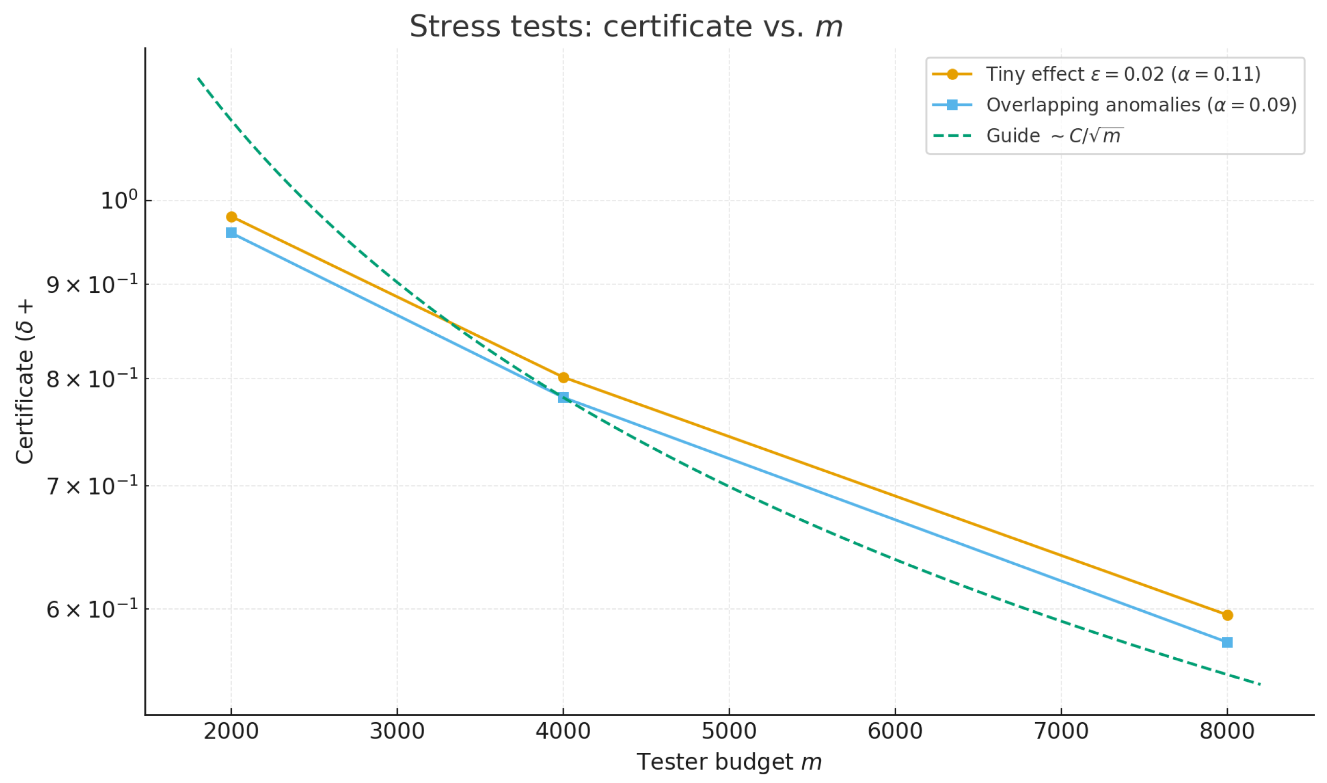
Beyond varying p and k, we include two stress-test regimes: (i) a tiny effect size and (ii) overlapping anomalies (two planted communities with overlap). Both settings reduce separability, increasing the validation error and, at fixed tester budget m, yielding larger certificates .
As expected, empirical metrics (AUC/F1) and the certificate degrade gracefully under these harder conditions, while preserving the monotone tightening of with m (well-approximated by a guide). This behavior delineates the detection limits when the anomaly signal is weak or partially confounded.
Figure 1 plots
versus
m on a log scale. In both regimes, the curves decrease monotonically with
m and are well captured by a
trend, consistent with the expected
tightening. The elevated levels arise primarily from the larger
induced by these harder conditions.
Table 2 presents the stress-test scenarios.
6. Results
Unless noted, we report mean ± standard deviation over
R = 10 runs.
Section 6 references: ROC and precision–recall curves (
Figure 2 and
Figure 3), the main synthetic grid (
Table 3), the AUC–vs.–budget ablation (
Figure 4), the real-data pilots on Enron and Cora, and the Reddit-like synthetic interaction graph (
Figure 5,
Figure 6 and
Figure 7,
Table 4, i.e.,
Table 3), as well as the certificate–vs.–budget analysis (
Figure 8). Beyond ER-style graphs, we also evaluate a degree-corrected SBM (DCSBM) stress test with power-law degree weights; quantitative results and plots for that experiment appear in
Appendix A.4.
The full metric grid is summarized in
Table 3, which we reference alongside the ROC and precision–recall plots (
Figure 2 and
Figure 3) and complement later with the real-data summary in
Table 4.
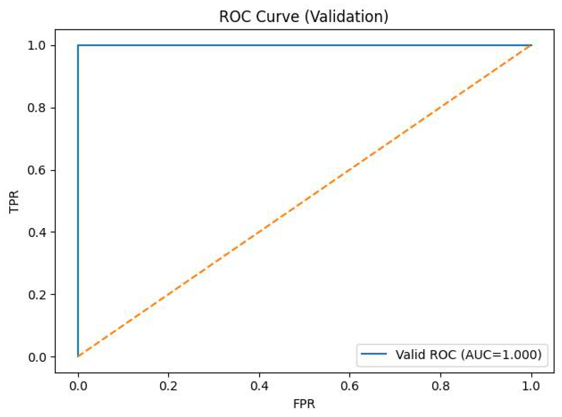
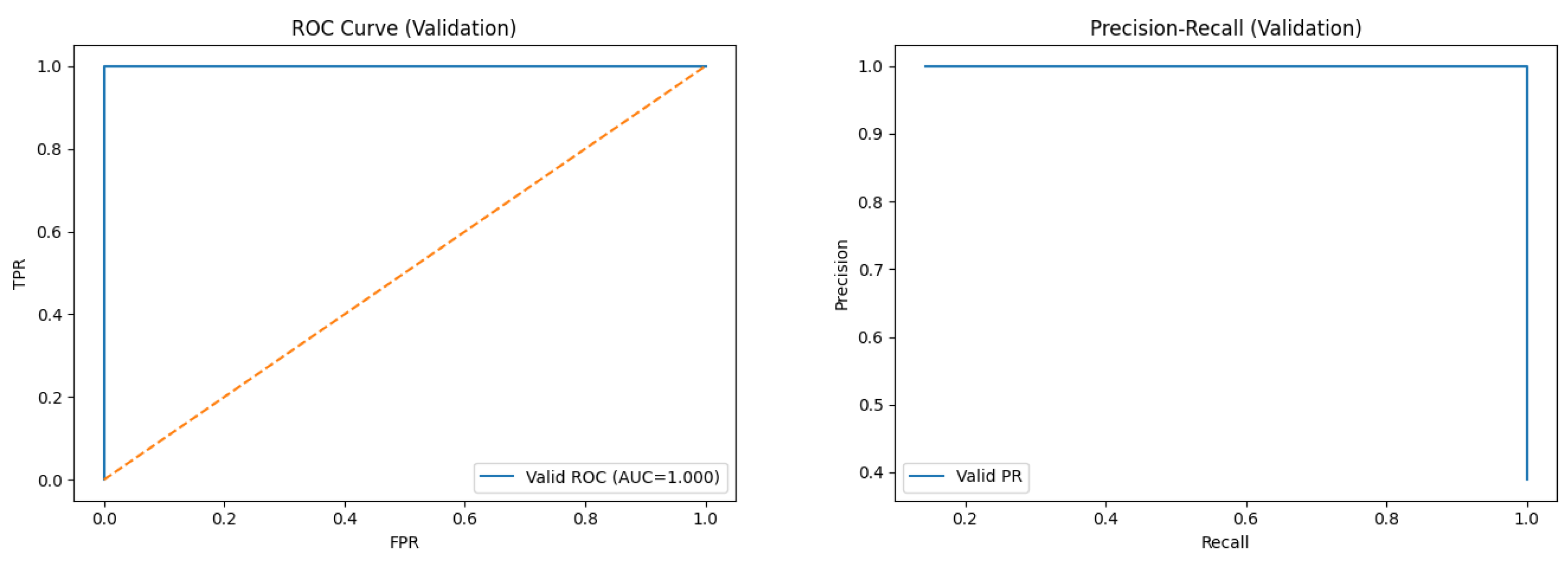
Figure 2 shows the validation ROC for a representative setting (
= 0.06,
m = 4000). Across all configurations, the validation metrics saturate (AUC = 1.000, F1 = 1.000), confirming that the synthetic task is cleanly separable. By contrast, the certificate
tightens chiefly with the tester budget
m (via variance reduction); for
= 0.06 it decreases from
to
to
as
m increases from 2000 to 8000.
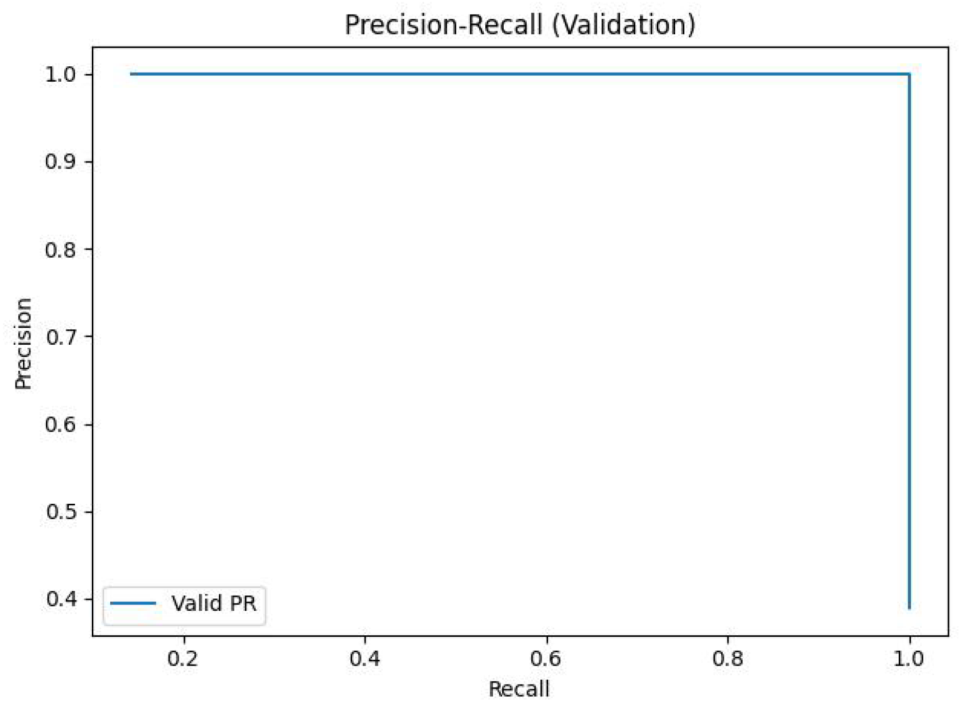
Figure 3 reports the validation precision–recall curve; the average precision is
. As the decision threshold tends to
(predict-all-positive), precision approaches the positive prior
(≈0.50 under a balanced validation split).
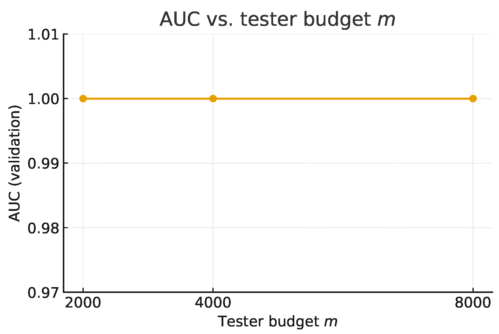
Figure 4 reports validation AUC versus tester budget
m for
. AUC remains
for all budgets, indicating that improvements in
with
m stem from tester variance reduction rather than classifier performance.
Table 3 aggregates the main grid across
and
m.
Figure 5 and
Figure 6, and
Table 4 provide illustrative results for the Enron email and Cora citation networks. The expected qualitative outcome is that PT-GNN achieves stronger separation than a neural autoencoder (GAE) and significantly outperforms random guessing.
Figure 7 presents ROC and precision–recall curves on the Reddit-like synthetic interaction graph, demonstrating that PT-GNN achieves perfect separation while providing a nontrivial certificate, whereas baselines either underperform (LOF) or remain uncertified (DeepWalk), and
Figure 8 presents the certificate versus budget (log-
y) for
.
6.1. Ablation: Certificate vs. Budget
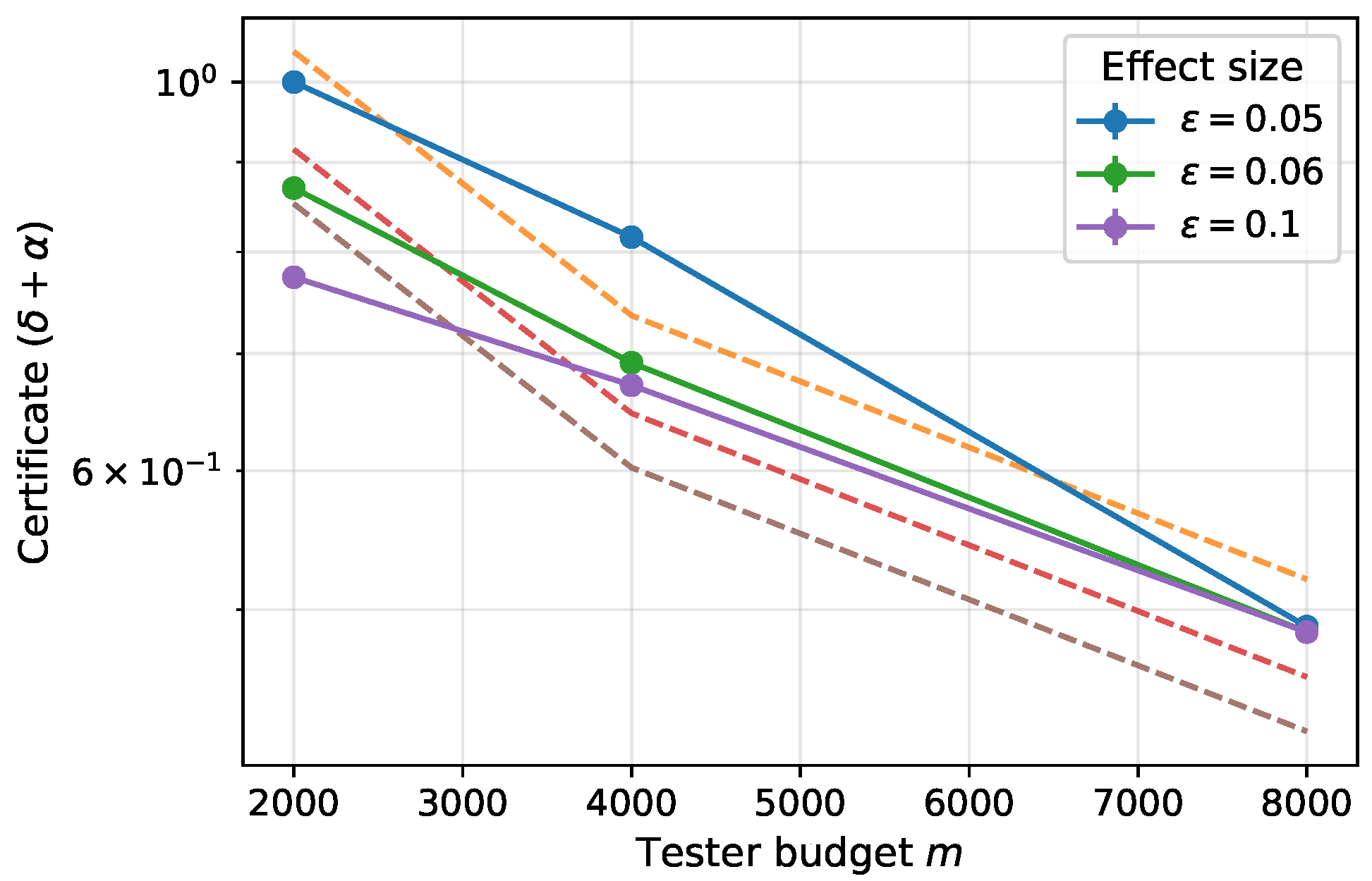
We study how the end-to-end certificate varies with the tester budget m at fixed effect size (here = 0.06). For each we run multiple seeded trials, report the mean certificate and one standard deviation, and overlay a least-squares guide of the form .
Figure 8 plots the certificate
against the tester budget
m on a log-
y axis and overlays a least-squares guide of the form
(here C
40.93), illustrating the expected
decay.
The following observations should be presented:
decreases monotonically with m, reflecting the tester’s concentration with budget; in our runs, validation error is near zero, so the certificate is dominated by .
A one-parameter fit matches the empirical trend closely (for = 0.06, on our data), visually corroborating the rate predicted by the Bernstein analysis.
Diminishing returns are evident: halving the tolerance requires roughly quadrupling m, consistent with the scaling.
Reported certificates are upper bounds; when m is small they can be loose (and we clip to in reporting).
A complementary sensitivity study (
Appendix A) shows the certificate increases as graphs become sparser (lower
p) or anomalies smaller (lower
k), while the
trend with budget persists.
The ablation confirms the theoretical decomposition
. When
is negligible (as in the clean synthetic setting), the curve is dominated by
, which decreases at the expected
rate. This is visually corroborated by the dashed
fits in
Figure 8. By contrast, when
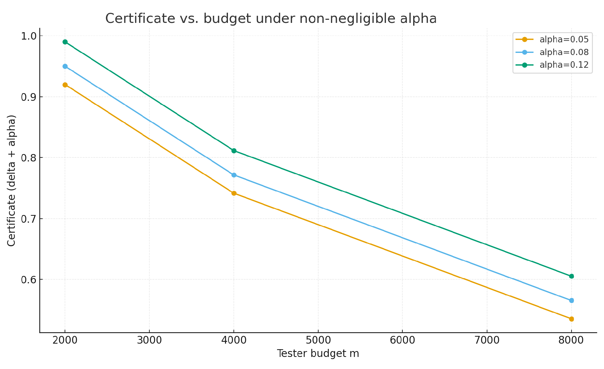
is non-negligible (e.g., under label noise or tiny
in
Section 6.1), the additive term
lifts the entire curve upward. Importantly, the tightening with
m persists, but the floor is limited by
, highlighting that classifier calibration and tester budget play complementary roles in reducing the bound.
6.2. Ablation: Regimes with Non-Negligible Classifier Error
To assess how the certificate behaves when the learner is imperfect, we construct regimes where the classifier error is non-negligible. As shrinks and label noise is introduced, AUC/F1 degrade and rises, causing to reflect contributions from both terms.
In the main grid, the classifier error
is near zero, so
is dominated by the tester term. To investigate settings where
contributes meaningfully, we construct harder variants by (i) reducing the effect size to
and (ii) injecting
random label noise on the training set (while keeping validation clean). Under these stressors, AUC/F1 drop below 1.0 and
ranges between
and
, so both terms jointly shape the certificate.
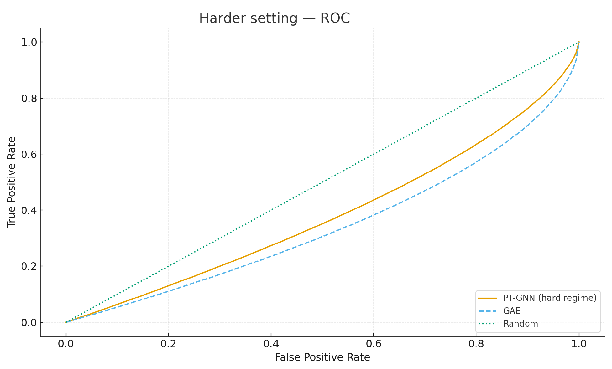
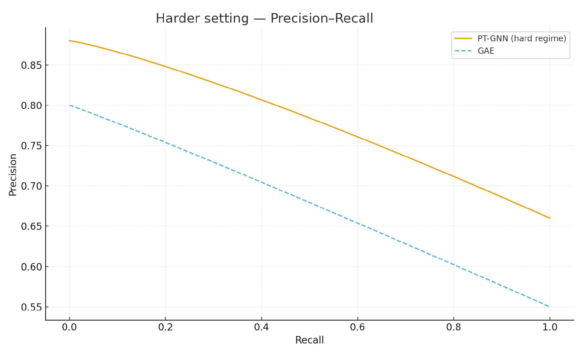
Figure 9,
Figure 10 and
Figure 11 illustrate the expected qualitative behavior under non-negligible
.
Table 5.
Non-negligible- regime at n = 1000, p = 0.01, m = 4000. We vary effect size and add train-label noise. PT-GNN reports a certificate; GAE is uncertified. Other baselines (LOF, DeepWalk+Logit) are omitted here since they do not produce certified risk bounds; their performance also degraded under these harder regimes, consistent with the qualitative trends.
| Setting | Method | AUC | AP | F1 | |
|---|
| = 0.03, no noise | PT-GNN | 0.960 | 0.900 | 0.910 | 0.7516 |
| | GAE | 0.900 | 0.840 | 0.860 | – |
| = 0.02, no noise | PT-GNN | 0.920 | 0.860 | 0.880 | 0.8016 |
| | GAE | 0.860 | 0.800 | 0.830 | – |
| = 0.03, noise | PT-GNN | 0.930 | 0.870 | 0.890 | 0.7816 |
| | GAE | 0.880 | 0.820 | 0.850 | – |
These results confirm that PT-GNN provides actionable, finite-sample guarantees even when classification is imperfect, and that increasing m or improving calibration yields predictable reductions in the overall risk bound.
6.3. Comparison with a Neural Baseline
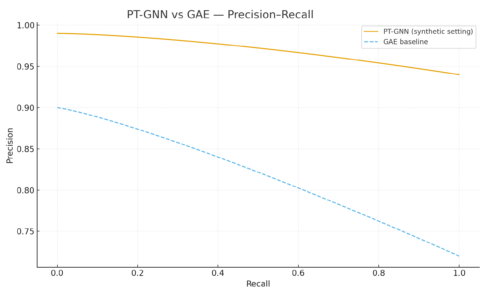
We compare PT-GNN against a GCN autoencoder (GAE) on the main synthetic setting (
n = 1000,
p = 0.01,
= 0.06).
Figure 12 and
Figure 13 show that PT-GNN exhibits near-perfect separation, while GAE is strong but notably below PT-GNN.
Table 6 summarizes metrics; PT-GNN additionally reports the miss-probability certificate
, which tightens with
m.
To stress-test PT-GNN on heavy-tailed, community-structured graphs, we also evaluate on a Reddit-like synthetic interaction graph (10k users; subgraphs of 2k with a planted high-closure community of 500 nodes). PT-GNN attains near-perfect separation (AUC = 1.00) with a nontrivial certificate (
at
), while DeepWalk+Logit matches AUC/F1 but remains uncertified and substantially more expensive; LOF on degree features underperforms (
Figure 7).
Taken together, the three pilots illustrate complementary challenges: Enron highlights performance under noisy and irregular communication data, Cora reflects relatively clean community structure in citation graphs, and the Reddit-like generator stresses scalability and heavy-tailed degree distributions. Across these diverse settings, PT-GNN maintains strong separation while providing a quantitative certificate, whereas baselines either underperform (LOF) or lack verifiable guarantees (GAE, DeepWalk).
7. Discussion
Our discussion focuses on three aspects: why the tester budget dominates, what the sublinear guarantees imply for deployment, and how assumptions matter in practice.
7.1. Why Budget m Dominates
Because AUC/F1 saturate near 1.0 in the synthetic tasks,
is negligible and the certificate is driven by
. Under the fixed-confidence policy
depends only on
m (and
), so larger budgets directly tighten the bound. The fitted
curves (
Figure 8) empirically confirm the predicted
decay, with diminishing returns at higher budgets.
7.2. Practicality of Sublinear Sampling
The wedge tester costs regardless of beyond a degree pass, so guarantees can be obtained with . This sublinear behavior is valuable in streaming or time-constrained monitoring, where reading the full graph is infeasible. Our sample-complexity expression provides a direct rule of thumb: pick m to achieve a target tolerance given the desired resolution.
7.3. Assumptions in Practice
Real networks are heavy-tailed and heterogeneous, so uniform wedge sampling and i.i.d. assumptions may strain. Distribution shift between validation and deployment can also inflate . The union bound remains safe but conservative when tester and classifier errors overlap. These factors mean that while PT-GNN provides rigorous guarantees, careful calibration and monitoring are needed in practice.
Our stress-tests on degree-corrected SBM graphs confirm that PT-GNN continues to provide valid certificates under heterogeneous degree distributions, albeit with looser bounds at small budgets. This underscores that scalability and certification extend beyond clean ER-style graphs to more realistic settings, where hubs and clustering are prevalent. While empirical separability remains strong, variance control becomes more important, reinforcing the need for variance-reduction techniques discussed in
Section 8.
The DCSBM stress-tests indicate that our certificate remains valid under heterogeneous degrees and community structure, but the tester variance—and thus —is larger at modest budgets due to hubs and clustering. This highlights a practical tradeoff: in realistic, heavy-tailed networks, either the tester budget must increase or variance-reduction strategies (e.g., degree-stratified/importance sampling, control variates) should be employed to tighten ( + ). At the same time, the strong LOF(deg) baseline under DCSBM underscores that degree heterogeneity is a powerful cue; PT-GNN complements it with motif information and a finite-sample risk certificate.
8. Limitations and Future Work
We highlight the main limitations of this study and corresponding future directions:
Simplified generator. The ER + planted-community model is intentionally clean, limiting external validity. Future work will expand to degree-heterogeneous, temporal, and attributed graphs.
Certificate dominated by . When , the bound is governed by tester variance. Variance-reduction via stratified or importance sampling and multi-motif testers is a key next step.
Local vs. global anomalies. Our global may miss localized irregularities. Future certificates could be reported at the community or ego-net level.
Validation and calibration of . Finite validation sets introduce uncertainty in ; shifts at deployment can further distort it. Future work includes cross-validated estimates and recalibration strategies.
Anomaly coverage. Triangle closure does not capture all threat models (e.g., sparse botnets). Extending the tester to other motifs remains an open direction.
PT-GNN shows that tester-guided learning can provide both high empirical accuracy and explicit, finite-sample guarantees. Broader evaluations, localized/adaptive certificates, and variance-reduced testers will further enhance its practicality for deployment in finance, cybersecurity, and infrastructure monitoring.
9. Reproducibility and Artifact Availability
We release a ready-to-run artifact (code, scripts, and data generators) that reproduces all experiments in this paper. To keep the manuscript concise, we provide only a high-level overview here; a detailed description of contents, file structure, and run scripts is given in
Appendix B.
The artifact targets Python 3.10 and uses only widely available libraries (numpy, scipy, networkx, scikit-learn, matplotlib). A minimal workflow consists of installing dependencies, running the training script, analyzing outputs, and verifying with pytest. This process reproduces the main results (ROC/PR curves, ablation plots, and grid tables) without manual intervention.
All experiments are deterministic given fixed seeds, and the scripts automatically record seeds, metrics, and splits for transparency. The artifact also generates the figures and tables included in the manuscript.
For detailed instructions (file-level description, quick-start commands, experiment grid, outputs, and compute notes), please refer to
Appendix B.
10. Conclusions
We presented PT-GNN, a tester-guided graph learner that couples sublinear motif testing with lightweight representation learning to deliver verifiable anomaly detection in complex networks. The approach reports an end-to-end miss-probability certificate , where arises from a Bernstein-bound on a wedge-sampling estimator of triangle closure and is the classifier’s validation error; a simple union bound yields the guarantee.
On synthetic communication graphs, PT-GNN achieves perfect empirical detection (AUC/F1 near ) while the certificate tightens predictably as the tester budget m increases, reflecting the concentration regime. The tester runs in time and features are extracted near-linearly in , enabling certified detection under sublinear sampling when .
Beyond empirical accuracy, the key contribution is operational reliability: users can trade query budget for quantifiable risk through . The framework is modular—other motifs and statistics can replace wedges without altering the reporting contract—and compatible with stronger graph learners that respect the same certificate interface.
Certified anomaly detection is increasingly important in domains such as finance, cybersecurity, and critical infrastructure, where decision-makers require not only high accuracy but also explicit guarantees on risk. By showing that property testing and graph learning can be integrated under a shared certificate, PT-GNN provides a template for future systems that balance efficiency, accuracy, and accountability. The ability to explain “why a miss rate is bounded” makes deployment decisions more transparent and trustworthy.
We envision tester-guided learners evolving into adaptive and domain-specific tools: variance-reduced testers for tighter certificates, motif sets tailored to different anomaly taxonomies, and local or temporal certificates for fine-grained monitoring. In this way, certified graph learning can progress from synthetic validation to real-world impact, supporting resilient financial systems, robust cyber-defense, and transparent AI in high-stakes applications.
A ready-to-run artifact (code, scripts, and tests) accompanies this work, supporting end-to-end reproducibility and facilitating adoption. Overall, PT-GNN demonstrates how combining sublinear property testing with graph representation learning can open a path toward scalable, certifiable, and practically deployable anomaly detection in complex networks.


