Strawberry Ripeness Detection Using Deep Learning Models

Abstract

In agriculture, the timely and accurate assessment of fruit ripeness is crucial to optimizing harvest planning and reduce waste. In this article, we explore the integration of two cutting-edge deep learning models, YOLOv9 and Swin Transformer, to develop a complex model for detecting strawberry ripeness. Trained and tested on a specially curated dataset, our model achieves a mean precision (mAP) of 87.3% by using the metric intersection over union (IoU) at a threshold of 0.5. This outperforms the model using YOLOv9 alone, which achieves an mAP of 86.1%. Our model also demonstrated improved precision and recall, with precision rising to 85.3% and recall rising to 84.0%, reflecting its ability to accurately and consistently detect different stages of strawberry ripeness.

1. Introduction

With global population growth, climate change, and the need for sustainable practices, the agricultural sector is facing unprecedented challenges that are in dire need of innovative solutions. Strawberries are highly perishable, sensitive to environmental conditions, and require precise harvest timing to ensure optimal quality and yield.

Fortunately, the use of AI and deep learning in agriculture is becoming more common. YOLOv9 is well known for its real-time target detection capabilities, while Swin Transformer excels at processing image data, especially for tasks requiring detailed visual understanding [1,2]. By integrating these two techniques for strawberry ripeness detection, we aim to significantly improve the accuracy and efficiency of detection, reduce reliance on manual labor, minimize human error, and make more accurate and timely harvest decisions.

The main objective of this article is how to effectively integrate and apply YOLOv9 and Swin Transformer technologies for strawberry ripeness detection, so the main research question of this article is as follows: How can we effectively combine YOLOv9 and Swin Transformer for strawberry ripeness detection? To solve this research question, we split it into the following questions:

• How can the integrated YOLOv9 and Swin Transformer model be trained and validated?
• What role does the Swin Transformer play in enhancing the accuracy of ripeness detection, and how does it complement the object detection capabilities of YOLOv9?
• How do we evaluate the model and prove that our improvements to the model are effective?

The core concept of this project is to utilize the complementary advantages of YOLOv9 and Swin Transformer to develop a robust, efficient, and highly accurate strawberry ripeness detection system. We train the dataset to obtain the best results and evaluate the model thoroughly.

This article is structured as follows: Section 2 reviews some of the related studies. Section 3 provides an in-depth discussion of the models and methods used in this research. Section 4 presents the results of the research. Section 5 concludes the article.

2. Related Work

Deep learning and computer vision have emerged as powerful tools in the field of agriculture, offering innovative solutions to various challenges faced in the industry. Various papers [3,4,5,6,7] present the status and applications of deep learning and computer vision in agriculture.

The effectiveness of using pretrained deep neural networks (DNNs) on agricultural datasets was explored to improve weed identification accuracy in precision agriculture [8].

The study by Sharma et al. [9] proposed the exceptional efficacy of convolutional neural networks (CNNs) in analyzing plant disease images. The faster R-CNN model they devised achieved a detection rate of 99.39% for chili plants, highlighting the potential of deep learning models to revolutionize agricultural disease management.

A method [10] was proposed to automatically detect unripe tomatoes by using a faster region-based convolutional neural network (faster R-CNN) and a ResNet-101 model to learn from the COCO dataset through transfer learning. The method performed well on immature and occluded tomatoes that are difficult to detect through traditional image analysis methods.

A CNN model [11] was introduced for the automated, lossless classification of mulberry maturity. The method improved the accuracy and efficiency of the sorting process by automatically classifying fruit into different ripeness categories based on visual cues.

Pardede et al. used the transfer learning ability of VGG-16 models for fruit ripeness detection. Their study [12] highlights the effectiveness of deep learning relative to traditional machine learning for this task, with a particular emphasis on the important role of regularization techniques in improving model performance.

A powerful CNN model was proposed by Momeny et al. [13] to detect citrus black spot disease and evaluate fruit ripeness through deep learning. One of their key innovations is the use of a learning augmentation strategy that generates new data from noisy and recovered images to enhance model training. Momeny et al. utilized Bayesian algorithm-optimized noise parameters to create noisy images and then took use of convolutional autoencoders to restore these images, effectively augmenting the training data.

We also studied research much more similar to ours.

Wang et al. [14] designed a model for strawberry detection and ripeness classification using the YOLOv8 model and image processing methods. Their research proved the feasibility and advantages of the YOLO model in researching strawberry ripeness detection.

Yang et al. [15] proposed a model combining YOLOv8 and LW-Swin Transformer. They used this model to detect the ripeness of strawberries. Their results showed that the combination of transformer and YOLO models outperformed the YOLO model.

In conclusion, it is very feasible to use deep learning for agricultural aspects, especially for fruit ripening detection. The potential of deep learning for fruit ripening detection represents an important step forward in agricultural technology, with the potential to not only reduce labor costs but also improve efficiency and reduce waste.

3. Materials and Methods

In this section, we outline the research methodology used for the development and evaluation of a deep learning-based system for the dynamic detection of strawberry ripeness through video analysis. The integration of YOLOv9 and Swin Transformer forms the core of our approach, and we leverage their capabilities to achieve real-time, accurate ripeness detection.

3.1. Research Design

3.1.1. Overview of the Proposed Model

In this article, we propose a strawberry ripeness detection method based on the YOLOv9 network and Swin Transformer. The method can automatically detect the position of strawberries from a video with multiple frames and track movement trajectory to mark the strawberries and predict their ripeness. This method will be a great convenience for growing and picking strawberries.

We trained a hybrid model by combining YOLOv9 and Swin Transformer, which enhanced the ability of this model to generalize and rely on modeling capabilities at a distance, resulting in better overall performance.

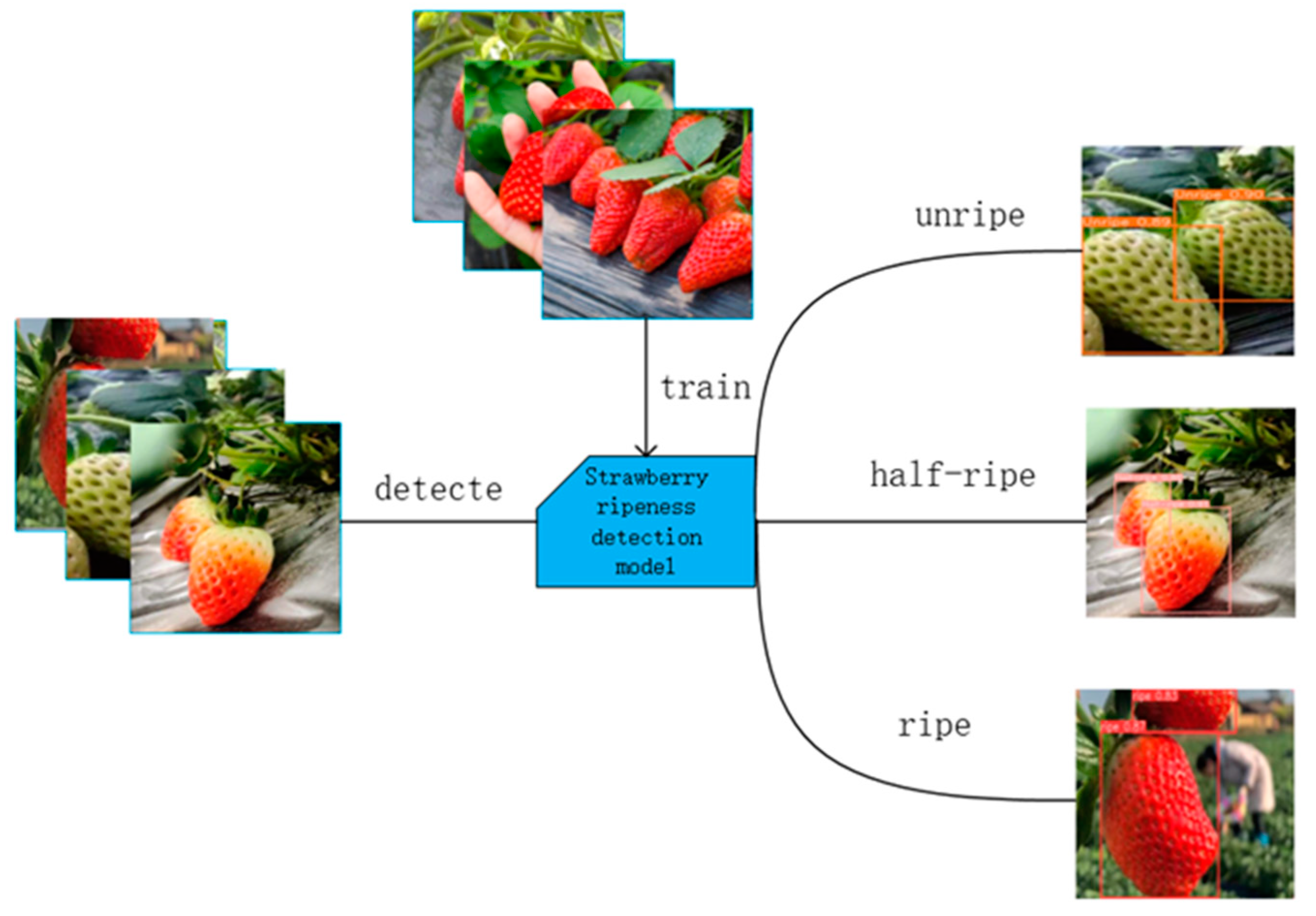
The overall structure of the strawberry ripeness detection model is shown in Figure 1. Firstly, the YOLOv9 model is trained by using the pre-prepared dataset. This model is improved by combining it with Swin Transformer, which can better extract the target feature information. Then, the video is processed by using a fusion network of YOLOv9 and Swin Transformer to detect strawberry ripeness with high accuracy. This model classifies the strawberries as “Unripe”, “Half-ripe”, and “Ripe”, outputting detection frames and feature vectors for each frame of the given video.

3.1.2. Research Design of the YOLOv9 Model

YOLOv9 introduces Programmable Gradient Information (PGI), which preserves important data throughout the depth of the proposed network, ensuring more reliable gradient generation and thus improving model convergence and performance. Meanwhile, YOLOv9 designs a new lightweight network structure based on gradient path planning: a generalized efficient layer aggregation network (GELAN). By using only conventional convolution, a GELAN achieves higher parameter utilization than deeply differentiable convolutional designs based on state-of-the-art techniques, while demonstrating the great advantages of being lightweight, fast, and accurate [16].

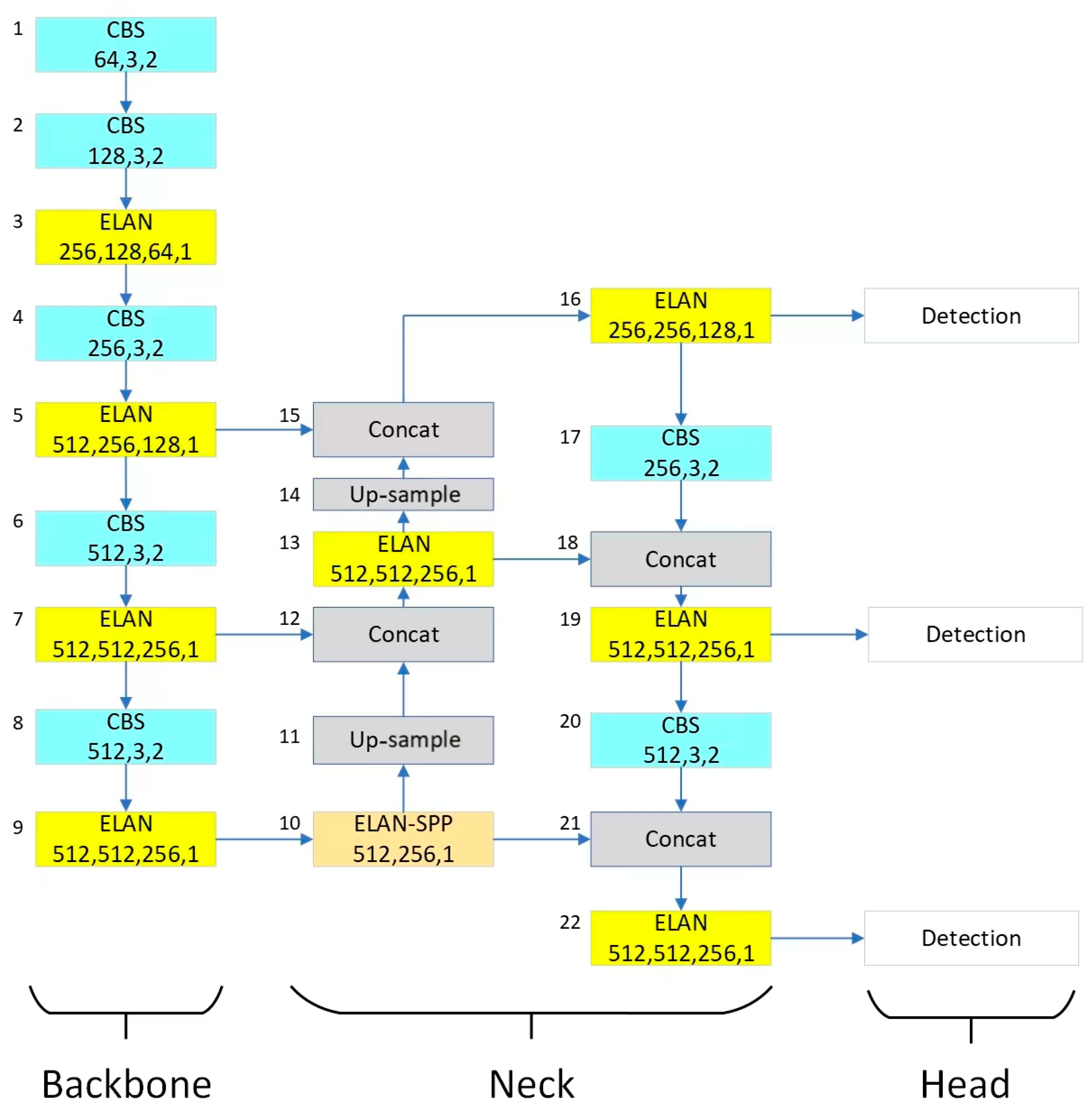
Figure 2 illustrates the convolutional neural network architecture of the YOLOv9 model. This model is divided into three main parts: Backbone, Neck, and Head. The Backbone is the main feature extraction part of this model. It consists of multiple convolutional layers that are responsible for extracting useful features from the input image. The Backbone consists of multiple layers that progressively reduce the spatial dimensions and increase the number of channels through different depth and step configurations, which helps in capturing features at different levels of abstraction in the image.

The Neck is the part that connects the Backbone and Head, which serves to perform feature fusion and realignment for object recognition. This part consists of upsampling and concat operations, which combine high-level, smaller-feature maps with low-level, larger-feature maps, thus preserving spatial information at different scales. This helps to detect objects at different scales of the image. The Head is the last part of the model and is responsible for object detection based on the features coming from the Backbone and Neck.

3.1.3. Research Design of Swin Transformer

Swin Transformer (Shifted Window Transformer) is a deep learning model based on transformers. Swin Transformer overcomes the problems of computational inefficiency and difficulty in handling high-resolution images which are found in traditional transformer models [17].

Figure 3 shows the structure of the Swin Transformer. At the beginning, the image is divided into multiple small blocks; each small block is usually a small square. These patches are flattened into vectors and passed into the model for processing. The model adopts a layered design and consists of four stages; each stage will reduce the resolution of the input feature map. The four stages build feature maps of varying sizes. The first stage goes through a Linear Embedding layer, and the next three stages go through a Patch Merging layer for downsampling. Swin Transformer Blocks are piled one after the other on each level.

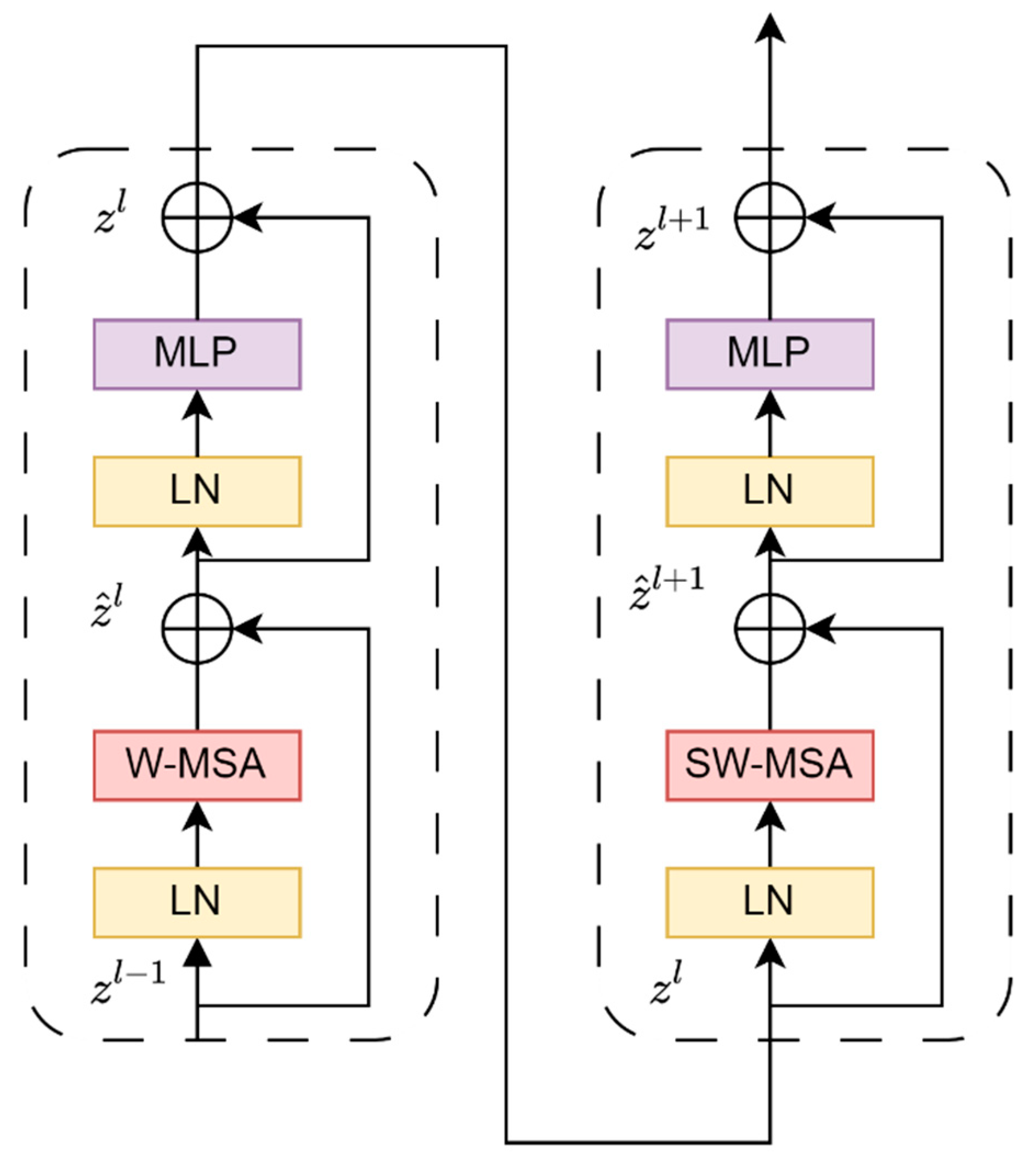
The transformer block has two structures, as shown in Figure 4. One structure makes use of the W-MSA structure, while the other uses the SW-MSA structure. A W-MSA structure and an SW-MSA structure are employed in pairs when utilizing these two structures.

As shown in Figure 5, assume that the input to Patch Merging is a 4 × 4 size single-channel feature map. Patch Merging will divide each 2 × 2 adjacent pixel into a patch, and then divide the same position in each patch. The same color pixels are put together to obtain four feature maps. These four feature maps are concat spliced in the depth direction, and then passed through a LayerNorm layer. Finally, a fully connected layer is used to make a linear change in the depth direction of the feature map, changing the depth of the feature map from C to C/2. In other words, after passing the Patch Merging layer, the height and width of the feature map will be halved, and the depth will be doubled.

Another important improvement of Swin Transformer is the window-based self-attention layer, which is abbreviated as W-MSA (Windows Multi-head Self-Attention). As shown in Figure 6, the left side is the ordinary Multi-head Self-Attention (MSA) module. Each pixel in the feature map needs to be calculated with all other pixels during the self-attention calculation process. When using the Windows Multi-head Self-Attention (W-MSA) module, first divide the feature map into windows according to the size of M × M (e.g., M = 2 in Figure 6), and then perform self-attention inside each window individually.

While using the W-MSA module, self-attention calculation will only be performed within each window, so information cannot be transferred between windows. To solve this problem, Swin Transformer introduces Shifted Windows Multi-head Self-Attention (SW-MSA).

In this article, we built the strawberry ripeness detection model based on YOLOv9. We propose a method to replace the backbone network in YOLOv9 with Swin Transformer. This hybrid model combines the fast and efficient detection capabilities of YOLOv9 with the powerful and flexible feature representation of Swin Transformer, designed to enhance the system’s ability to accurately identify and classify strawberry ripeness from video input.

In the hybrid model, Swin Transformer acts as a powerful feature extractor by capturing the details and variations in strawberry appearance. These details and changes mark different stages of maturity. Swin Transformer ensures that global and local features are effectively captured and used for prediction. This is particularly useful for detecting strawberries under varying lighting, occlusion, and background complexity conditions.

3.2. Data Preparation

In this article, we collected various strawberry images, videos, and datasets to ensure the quality and accuracy of our models. For the dataset, we used pre-processing techniques such as image cropping, resizing, and labeling to ensure that the dataset was processed into the form required by the model.

We downloaded test videos of strawberry plantations from the Internet and performed image extraction on the videos. We used a Python (version: 3.13) script to assist us in extracting images. This script allowed us to split the video into images at set intervals. This was helpful for reducing data redundancy. Additionally, we downloaded strawberry images from the Internet to increase robustness.

As shown in Figure 7, we collected a total of 722 strawberry images. In addition, we also downloaded the open source strawberry image dataset of the StrawDI team and selected images that met our requirements [18]. Finally, we collected a total of 2000 strawberry images from different regions and under different lighting and weather conditions, which helped to enhance model diversity.

In this article, we used EISeg (version 1.1.1) to label the collected strawberry images. Figure 8 illustrates the results after labeling. EISeg (Efficient and Interactive Segmentation) is an efficient interactive image segmentation tool, mainly used in geospatial analysis, remote sensing image processing, medical image processing, and other fields. EISeg provides a method with which to achieve precise segmentation with minimal user interaction, greatly improving the efficiency and accuracy of image segmentation [19].

Data splitting is a fundamental method in machine learning for training models and evaluating model performance. It involves dividing the dataset into separate subsets to provide an honest assessment of the performance of proposed models using unseen data. The three main subsets commonly used are the training dataset, validation dataset, and test dataset. The training set is the largest part of the dataset used to train the model. The validation set is employed to provide an unbiased assessment of the model which fits on the training dataset when adjusting the model’s hyperparameters. After the model has been trained and validated, the test set is used for an unbiased evaluation of the final model. Correct data splitting can avoid model overfitting problems and significantly improve the validity and reliability of model evaluation.

In this article, we also split the data. We make use of 80% of the dataset for training, 10% for validation, and 10% for testing. Figure 9 clearly illustrates the dataset splitting.

3.3. Evaluation Methods

Evaluation is a critical step for computer vision models, one which helps to measure model performance and guide future improvements. In deep learning, all evaluation methods are based on a confusion matrix.

Table 1. Confusion matrix.

	Positive	Negative
True	TP	TN
False	FP	FN

shows the confusion matrix. In Table 1, True Positive (TP) means that the true category of the sample is a positive sample and the model predicts it as a positive sample; therefore, the prediction is correct. True Negative (TN) means that the true category of the sample is a negative example and the model predicts it as a negative example; therefore, the prediction is correct. False Positive (FP) is a sample whose true category is a negative sample, but the model predicts it as a positive sample; and therefore, the prediction is wrong. False Negative (FN) means that the true category of the sample is a positive example, but the model predicts that it as a negative example, and so the prediction is wrong [20].

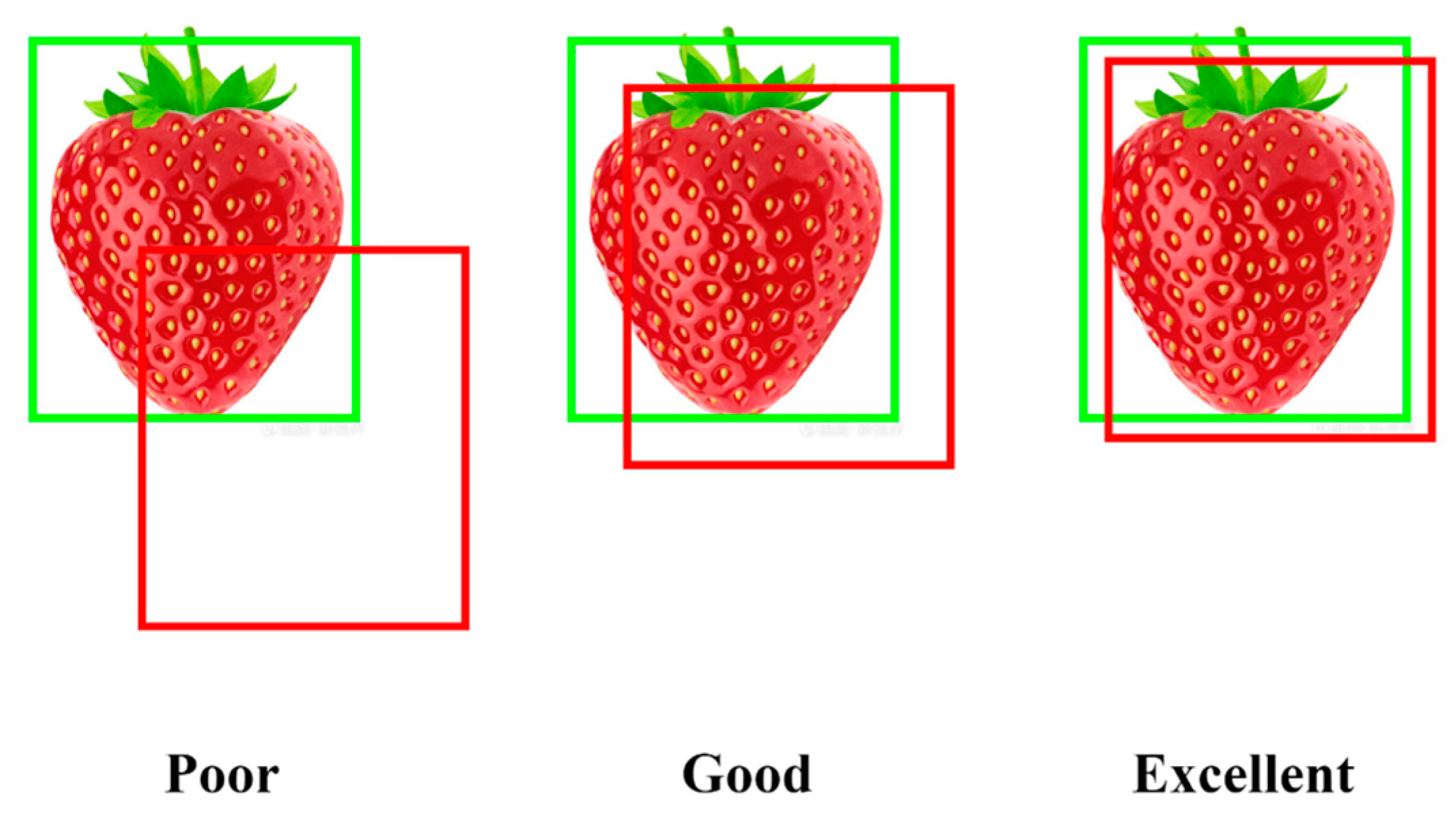
IoU (intersection over union) is a general evaluation index in the field of computer vision, especially in tasks such as target detection and image segmentation. IoU mainly reflects the degree of overlap between the predicted bounding box and the ground truth bounding box. As shown in Figure 10, the green box is the truth bounding box, which is the box marked while labeling the dataset. The red box is the predicted bounding box, which is the one predicted by the trained model. IoU is the result of dividing the overlapping part of two areas by the area of union of the two areas [21].

$$\mathrm{I}\mathrm{o}\mathrm{U}={\displaystyle \frac{\mathrm{A}\mathrm{r}\mathrm{e}\mathrm{a} \mathrm{o}\mathrm{f} \mathrm{O}\mathrm{v}\mathrm{e}\mathrm{r}\mathrm{l}\mathrm{a}\mathrm{p}}{\mathrm{A}\mathrm{r}\mathrm{e}\mathrm{a} \mathrm{o}\mathrm{f} \mathrm{U}\mathrm{n}\mathrm{i}\mathrm{o}\mathrm{n}}}$$

(1)

Precision is an indicator in evaluating the performance of a classification model. It measures the proportion of items that the model correctly identifies as positive out of all items that the model identifies as positive [22].

$$\mathrm{P}\mathrm{r}\mathrm{e}\mathrm{c}\mathrm{i}\mathrm{s}\mathrm{i}\mathrm{o}\mathrm{n}={\displaystyle \frac{\mathrm{T}\mathrm{P}}{\mathrm{T}\mathrm{P}+\mathrm{F}\mathrm{P}}}$$

(2)

Although precision is an important metric, it does not provide a complete view of model performance on its own. Therefore, precision is often combined with recall

$$\mathrm{R}\mathrm{e}\mathrm{c}\mathrm{a}\mathrm{l}\mathrm{l}={\displaystyle \frac{\mathrm{T}\mathrm{P}}{\mathrm{T}\mathrm{P}+\mathrm{F}\mathrm{N}}}$$

(3)

where mAP (mean average precision) is an indicator to widely evaluate model performance in computer vision tasks, especially in the fields of target detection and image retrieval. The mAP provides a single performance metric to evaluate the overall effectiveness of the model by comprehensively considering the precision and recall of the model under different categories and different detection difficulties. By plotting the curve of precision versus recall and calculating the area under the curve (AUC), the AP value of a single category is obtained. The mAP value is the average of the AP values of all categories. The higher the value, the better the performance of the model. The mathematical expressions are shown in Equations (4) and (5). In this article, the prediction results are divided into three classes, namely, k = 3

$$\mathrm{A}\mathrm{P}={\int }_0^1\mathrm{p}\left(\mathrm{r}\right)\mathrm{d}\mathrm{r}$$

(4)

$$\mathrm{m}\mathrm{A}\mathrm{P}={\displaystyle \frac{{\sum }_{\mathrm{i}=1}^{\mathrm{k}}\mathrm{A}{\mathrm{P}}_{\mathrm{i}}}{\mathrm{k}}}$$

(5)

where mAP@IoU represents the mAP value calculated under a specific IoU threshold. For example, mAP@0.5 means that the result is considered correct only when IoU ≥ 0.5. mAP@0.5 is a very popular evaluation metric because it considers the recognition accuracy and positioning accuracy of the model. mAP@[0.5:0.95] is also an evaluation indicator, which calculates the average of all mAP values with IoU from 0.5 to 0.95 (in steps of 0.05). This approach is more rigorous as it considers a range of different IoU thresholds, providing a more comprehensive perspective on model performance.

4. Results

4.1. Performance of Strawberry Ripeness Detection Model

Figure 11 shows the results of our model based on the validation dataset. In the same validation dataset, our model can detect most strawberries of different sizes, orientations, environments, and degrees of ripeness.

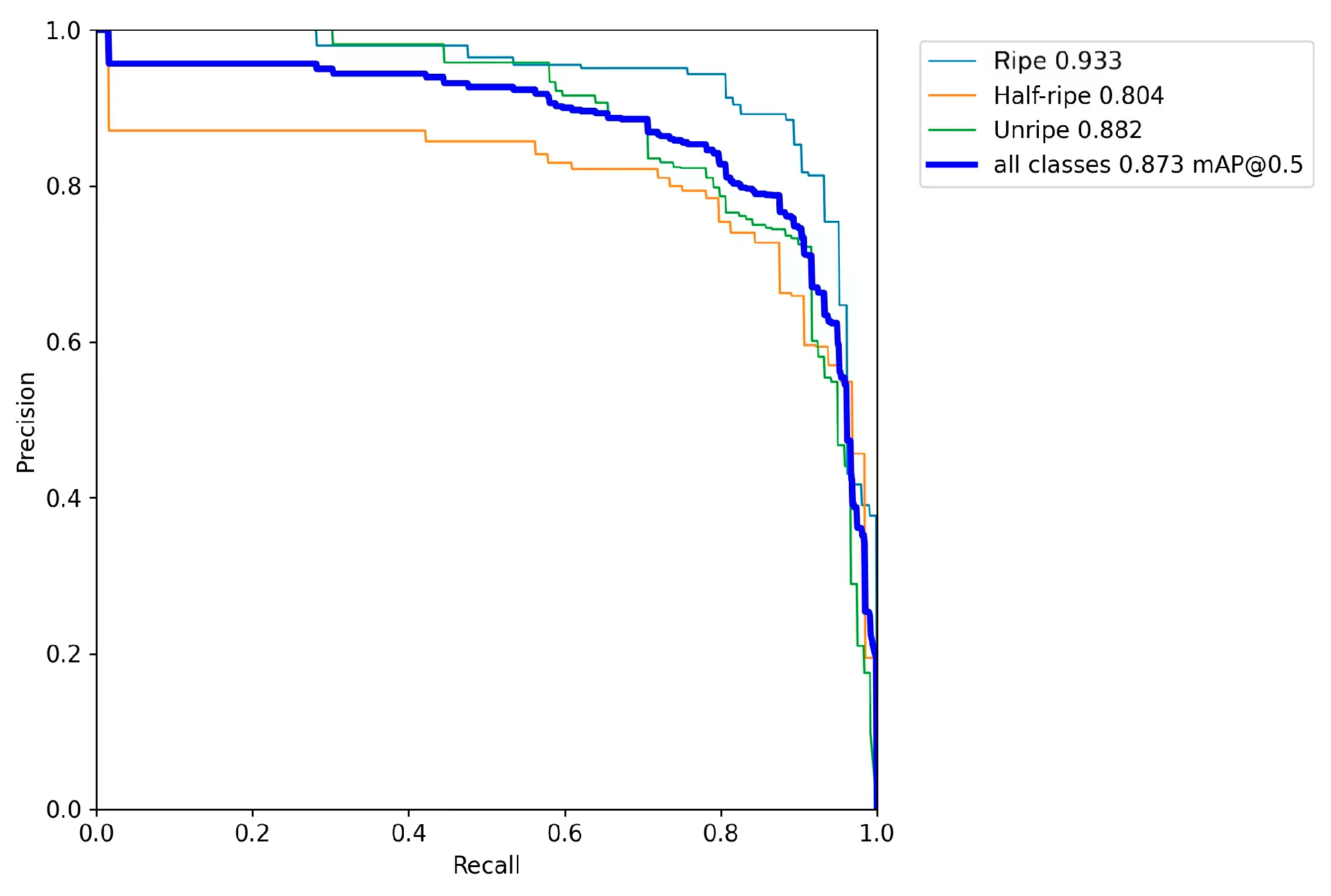
To evaluate the performance of our model, we plotted the precision–recall (PR) curves for both the YOLOv9+Swin Transformer model and the YOLOv9 model, as shown in Figure 12 and Figure 13. The PR curve demonstrates the trade-off between precision and recall, with the thin lines representing the PR curves for each category and the thick line representing the average PR curve across all categories. The area under the PR curve (AUC) provides a measure of model performance [23]:

• For “ripe” strawberries, the AUC increased from 0.925 to 0.933;
• For “half-ripe” strawberries, the AUC increased from 0.789 to 0.804;
• For “unripe” strawberries, the AUC increased from 0.868 to 0.882;
• The overall AUC of mAP@0.5 improved from 0.861 to 0.873.

These improvements demonstrate that the YOLOv9+Swin Transformer model outperforms the YOLOv9 model in all ripeness categories, with higher precision and recall values.

The evaluation metrics for the proposed model are shown in Figure 14. The high and stable precision and recall values indicate that the model performs well. The mAP@0.5 and mAP@[0.5:0.95] values continue to increase, reflecting the model’s robustness under different levels of detection stringency. Overall, the model shows improvement over time in all aspects: bounding box prediction, object presence confidence, and classification.

From

Table 2. Comparison of strawberry ripeness detection models.

Model	Precision	Recall	mAP@0.5	mAP@[0.5:0.95]
YOLOv9	0.777	0.800	0.861	0.610
YOLOv8	0.774	0.749	0.823	0.552
YOLOv8+Swin Transformer	0.815	0.831	0.861	0.613
YOLOv9+Swin Transformer	0.853	0.840	0.873	0.627

, we can analyze the performance of different versions of the YOLO model in terms of precision, recall, and mAP. The YOLOv9+Swin Transformer model has the highest precision, reaching 0.853. In comparison, the precision of the original YOLOv8 and YOLOv9 is slightly lower, with YOLOv9 being 0.777 and YOLOv8 being 0.774. YOLOv9+Swin Transformer reaches 0.840 in recall, higher than the other three models. YOLOv9+Swin Transformer also has the highest mAP@0.5, reaching 0.873. On the more stringent mAP@[0.5:0.95], YOLOv9+Swin Transformer also showed the best performance, reaching 0.627. In summary, the YOLOv9+Swin Transformer model we proposed performs optimally on all major performance indicators. This further demonstrates that our method combining YOLOv9 and Swin Transformer is able to improve the performance of the strawberry detection model.

All in all, our strawberry ripeness detection model can accurately detect the ripeness of strawberries. All the indicators of the model are very good, and our improvements to the model have proven to be very effective.

4.2. Comparison of YOLOv10 Model

YOLOv10 introduces a new approach to real-time target detection. Addressing the shortcomings of previous versions of YOLO in terms of post-processing and model architecture, YOLOv10 achieves state-of-the-art performance while significantly reducing computational overhead [1]. We also tested our dataset on the YOLOv10 model. The results are shown in

Table 3. Comparison of YOLOv10 model.

Model	Precision	Recall	mAP@0.5	mAP@[0.5:0.95]
YOLOv9	0.777	0.800	0.861	0.610
YOLOv10	0.817	0.789	0.871	0.620
YOLOv9+Swin Transformer	0.853	0.840	0.873	0.627

.

While YOLOv10 shows an improved performance compared to YOLOv9, the combination of YOLOv9 with Swin Transformer still achieves the highest scores. This suggests that while the enhancements introduced in YOLOv10 are beneficial, the integration with Swin Transformer provides the best results for real-time target detection. Notably, YOLOv10 also significantly reduces training time, suggesting potential for further improvements by combining YOLOv10 with transformer models to balance efficiency and accuracy.

5. Conclusions and Future Work

5.1. Analysis and Discussions

In summary, the model of YOLOv9 and Swin Transformer effectively improves the accuracy and reliability of strawberry ripeness detection. Indicators such as precision, recall, and mAP all show that the hybrid model of YOLOv9 and Swin Transformer has better detection results for strawberries of various ripeness levels.

As shown in the previous sections, our experimental results show that the hybrid model of YOLOv9 and Swin Transformer performs better than the YOLOv9 model. The key factors enabling these advances include the following:

Firstly, Swin Transformer can capture detailed and subtle features of strawberries, which greatly improves detection rates. This works particularly well in complex scenes where strawberries appear under various lighting and occlusion conditions.

Secondly, the architecture of YOLOv9, especially the integration of Programmable Gradient Information (PGI) and its lightweight and powerful network structure (GELAN), can locate strawberries quickly and accurately within video frames.

5.2. Conclusions

In this research project, we successfully demonstrated the integration of YOLOv9 and Swin Transformer models to detect strawberry ripeness with high accuracy. The hybrid model achieved a mean average precision (mAP) at an IoU of 0.5 of 87.3%, surpassing the performance of traditional models using YOLOv9 alone, which registered an mAP of 86.1%. The precision and recall are better. This improvement underscores the effectiveness of combining these advanced deep learning technologies to enhance precision in agricultural applications. The ability of this proposed model to accurately categorize strawberries into unripe, half-ripe, and ripe stages can significantly aid in optimizing harvest times, thus reducing waste and increasing yield quality.

5.3. Limitations

While the results are promising, our research has several limitations:

Firstly, though the dataset includes images of strawberries from a variety of conditions, they are primarily of one variety. This limitation may affect the applicability of the model to different varieties of strawberries, such as strawberries that are white when ripe.

Secondly, our model has good performance. However, the performance of this proposed model in actual strawberry planting may be affected by external factors such as lighting and camera clarity.

Finally, the strawberry dataset we have proposed is limited in size and variety, and using more datasets may further improve model performance.

5.4. Future Work

Our future research will be to solidify the findings of this article and address its limitations.

Firstly, we will collect and integrate data from a wider range of climates and geographic regions to improve the model’s robustness and applicability in different agricultural settings.

Secondly, we will improve the model according to different varieties of strawberries to improve the general applicability of our model in relation to various varieties of strawberries.

Thirdly, we will combine visual data with input from environmental sensors (e.g., humidity, temperature), which can improve the accuracy of maturity detection under different environmental conditions.

Finally, we will try to train a model that combines YOLOv10 and transformer to achieve improved detection results while being more lightweight.

References

- Wang, A.; Chen, H.; Liu, L.; Chen, K.; Lin, Z.; Han, J.; Ding, G. YOLOv10: Real-Time End-to-End Object Detection. arXiv 2024, arXiv:2405.14458. [Google Scholar]
- Liu, Z.; Lin, Y.; Cao, Y.; Hu, H.; Wei, Y.; Zhang, Z.; Lin, S.; Guo, B. Swin transformer: Hierarchical vision transformer using shifted windows. In Proceedings of the IEEE/CVF International Conference on Computer Vision, Montreal, BC, Canada, 11–17 October 2021; pp. 10012–10022. [Google Scholar]
- Dhanya, V.G.; Subeesh, A.; Kushwaha, N.L.; Vishwakarma, D.K.; Kumar, T.N.; Ritika, G.; Singh, A.N. Deep learning based computer vision approaches for smart agricultural applications. Artif. Intell. Agric. 2022, 6, 211–229. [Google Scholar] [CrossRef]
- Fracarolli, J.A.; Pavarin, F.F.A.; Castro, W.; Blasco, J. Computer vision applied to food and agricultural products. Rev. Ciência Agronômica 2020, 51, e20207749. [Google Scholar] [CrossRef]
- Ghazal, S.; Munir, A.; Qureshi, W.S. Computer vision in smart agriculture and precision farming: Techniques and applications. Artif. Intell. Agric. 2024, 13, 64–83. [Google Scholar] [CrossRef]
- Kamilaris, A.; Prenafeta-Boldú, F.X. Deep learning in agriculture: A survey. Comput. Electron. Agric. 2018, 147, 70–90. [Google Scholar] [CrossRef]
- Bharman, P.; Saad, S.A.; Khan, S.; Jahan, I.; Ray, M.; Biswas, M. Deep learning in agriculture: A review. Asian J. Res. Comput. Sci. 2022, 13, 28–47. [Google Scholar] [CrossRef]
- Espejo-Garcia, B.; Mylonas, N.; Athanasakos, L.; Fountas, S.; Vasilakoglou, I. Towards weeds identification assistance through transfer learning. Comput. Electron. Agric. 2020, 171, 105306. [Google Scholar] [CrossRef]
- Sharma, R.; Kukreja, V.; Bordoloi, D. Deep learning meets agriculture: A faster RCNN based approach to pepper leaf blight disease detection and multi-classification. In Proceedings of the 2023 4th International Conference for Emerging Technology (INCET), Belgaum, India, 26–28 May 2023; pp. 1–5. [Google Scholar]
- Mu, Y.; Chen, T.S.; Ninomiya, S.; Guo, W. Intact detection of highly occluded immature tomatoes on plants using deep learning techniques. Sensors 2020, 20, 2984. [Google Scholar] [CrossRef] [PubMed]
- Ashtiani, S.-H.M.; Javanmardi, S.; Jahanbanifard, M.; Martynenko, A.; Verbeek, F.J. Detection of mulberry ripeness stages using deep learning models. IEEE Access 2021, 9, 100380–100394. [Google Scholar] [CrossRef]
- Pardede, J.; Sitohang, B.; Akbar, S.; Khodra, M.L. Implementation of transfer learning using VGG16 on fruit ripeness detection. Int. J. Intell. Syst. Appl. 2021, 13, 52–61. [Google Scholar] [CrossRef]
- Momeny, M.; Jahanbakhshi, A.; Neshat, A.A.; Hadipour-Rokni, R.; Zhang, Y.-D.; Ampatzidis, Y. Detection of citrus black spot disease and ripeness level in orange fruit using learning-to-augment incorporated deep networks. Ecol. Inform. 2022, 71, 101829. [Google Scholar] [CrossRef]
- Wang, C.; Wang, H.; Han, Q.; Zhang, Z.; Kong, D.; Zou, X. Strawberry Detection and Ripeness Classification Using YOLOv8+ Model and Image Processing Method. Agriculture 2024, 14, 751. [Google Scholar] [CrossRef]
- Yang, S.; Wang, W.; Gao, S.; Deng, Z. Strawberry ripeness detection based on YOLOv8 algorithm fused with LW-Swin Transformer. Comput. Electron. Agric. 2023, 215, 108360. [Google Scholar] [CrossRef]
- Bakirci, M.; Bayraktar, I. YOLOv9-Enabled Vehicle Detection for Urban Security and Forensics Applications. In Proceedings of the 2024 12th International Symposium on Digital Forensics and Security (ISDFS), San Antonio, TX, USA, 29–30 April 2024; pp. 1–6. [Google Scholar]
- Liu, Z.; Ning, J.; Cao, Y.; Wei, Y.; Zhang, Z.; Lin, S.; Hu, H. Video Swin Transformer. In Proceedings of the IEEE/CVF Conference on Computer Vision and Pattern Recognition (CVPR), New Orleans, LA, USA, 18–24 June 2022; pp. 3192–3201. [Google Scholar]
- Pérez-Borrero, I.; Marín-Santos, D.; Gegúndez-Arias, M.E.; Cortés-Ancos, E. A fast and accurate deep learning method for straw-berry instance segmentation. Comput. Electron. Agric. 2020, 178, 105736. [Google Scholar] [CrossRef]
- Xian, M.; Xu, F.; Cheng, H.D.; Zhang, Y.; Ding, J. EISeg: Effective interactive segmentation. In Proceedings of the International Conference on Pat-tern Recognition (ICPR), Cancun, Mexico, 4–8 December 2016; pp. 1982–1987. [Google Scholar]
- Caelen, O. A Bayesian interpretation of the confusion matrix. Ann. Math. Artif. Intell. 2017, 81, 429–450. [Google Scholar] [CrossRef]
- Everingham, M.; Van Gool, L.; Williams, C.K.I.; Winn, J.; Zisserman, A. The Pascal Visual Object Classes (VOC) Challenge. Int. J. Comput. Vis. 2010, 88, 303–338. [Google Scholar] [CrossRef]
- Buckland, M.; Gey, F. The relationship between Recall and Precision. J. Am. Soc. Inf. Sci. 1994, 45, 12–19. [Google Scholar] [CrossRef]
- Davis, J.; Goadrich, M. The relationship between Precision-Recall and ROC curves. In Proceedings of the 23rd International Conference on Machine Learning (ICML), Pittsburgh, PA, USA, 25–29 June 2006; ACM Press: New York, NY, USA, 2006; pp. 233–240. [Google Scholar]