Improving Machine Learning Predictive Capacity for Supply Chain Optimization through Domain Adversarial Neural Networks

Abstract

In today’s dynamic business environment, the accurate prediction of sales orders plays a critical role in optimizing Supply Chain Management (SCM) and enhancing operational efficiency. In a rapidly changing, Fast-Moving Consumer Goods (FMCG) business, it is essential to analyze the sales of the products and accordingly plan the supply. Due to low data volume and complexity, traditional forecasting methods struggle to capture intricate patterns. Domain Adversarial Neural Networks (DANNs) offer a promising solution by integrating transfer learning techniques to improve prediction accuracy across diverse datasets. This study presents a new sales order prediction framework that combines DANN-based feature extraction and various machine learning models. The DANN method generalizes the data, maintaining the data behavior’s originality. The approach addresses challenges like limited data availability and high variability in sales behavior. Using the transfer learning approach, the DANN model is trained on the training data, and this pre-trained DANN model extracts relevant features from unknown products. In contrast, Machine Learning (ML) algorithms are used to build predictive models based on it. The hyperparameter tuning of ensemble models such as Decision Tree (DT) and Random Forest (RF) is also performed. Models like the DT and RF Regressor perform better than Linear Regression and Support Vector Regressor. Notably, even without hyperparameter tuning, the Extreme Gradient Boost (XGBoost) Regressor model outperforms all the other models. This comprehensive analysis highlights the comparative benefits of various models and establishes the superiority of XGBoost in predicting sales orders effectively.

1. Introduction

Forecasting-based supply chain optimization is necessary for organizations seeking to boost effectiveness and production, minimize expenses, and improve their overall performance. Forecasting helps organizations predict changes in an entity’s market and optimize their supply chain operations by analyzing them with an understanding of future demand patterns [1]. Organizations can manage inventory levels, improve production schedules, and reduce inventory shortages by accurately forecasting demand. With an organized approach, supply chain disruption risks like supplier delays and unexpected demands can be minimized [2,3]. Forecasting also promotes better use of resources, waste reduction, and sustainability. Businesses can gain a competitive edge by promoting flexibility and adjusting to varying market conditions by using historical data and advanced analytics approaches to improve the accuracy and dependability of forecasting models. A Fast-Moving Consumer Goods (FMCG) company needs to analyze data, predict or forecast demand, and adapt the planning framework for better demand forecasts and enhanced sales.

Data scarcity (Insufficient information) is a significant challenge in a supply chain field due to scattered systems, inconsistent standards, limited connectivity, and security concerns [4]. Companies need to improve visibility and accuracy by collecting, organizing, and analyzing data from internal and external sources to address this. Standardizing data formats and consolidating information from various sources are crucial for optimizing operations. Using cutting-edge technologies like blockchain, RFID tags, and Internet of Things (IoT) sensors can create new data streams and enable real-time tracking, enhancing supply chain transparency and efficiency. Investing in these capabilities promotes innovation, efficiency, and competitiveness in the supply chain field, where demand prediction can impact decision-making.

The data-driven forecasting of demand for a product is crucial for understanding the relationships between production, distribution, and sales elements, enabling FMCG businesses to optimize operational efficiency, enhance customer satisfaction, and drive down costs. Here in this study, the SupplyGraph dataset is utilized to predict sales. In this dataset, high variability in data distribution makes it difficult to predict the target variable. Machine Learning (ML) models often struggle to predict accurately in scenarios with high data variability and small population sizes. This is due to the limited amount of data available for training, which can introduce complexities in understanding the nature of data by the model [5]. This results in poor generalization and an inability to predict outcomes in real-world scenarios. The limited sample size may not accurately represent the full spectrum of variability in the data. To address these inefficiencies, careful consideration of data collection strategies, feature engineering techniques, and model selection is required. Feature engineering and better model selection are implemented to overcome this challenge.

Tackling the fluctuations in datasets is essential, and it can be achieved through the Domain-Adversarial Neural Network (DANN) model used here. DANN is a model architecture that uses a domain adaptation approach to achieve data augmentation and generalization. It comprises a feature extractor, a label predictor, and a domain classifier. The feature extractor learns to extract features from input data, which are then used by the label predictor and domain classifier. The label predictor predicts the target variable, while the domain classifier classifies the data origin. DANN optimizes the feature extractor to minimize prediction error, aligning feature representations across domains. This results in more robust and generalizable representations, improving performance in product sales prediction and logistics planning tasks. DANN indirectly augments the dataset by enabling better generalization to unseen data from diverse domains.

Variability in data, which can frequently come due to product categories, customers, production, and demand, can create problems that are difficult for traditional forecasting models to analyze correctly. Organizations may overcome these obstacles and gain better generalization across several domains by adding domain labels to the forecasting task using the DANN model. In this proposed approach, a DANN is used to generalize and understand the data better, resulting in better forecasting. Using transfer learning, the strategically combined weights of the training data are used to test data to forecast the selected products. By concatenating the weights and transfer learning approach, the DANN model blends time series information with domain labels, allowing the model to learn the complicated relationships between these features and labels. Using this method, the model may identify patterns or variations unique to a particular domain within the dataset.

Through data generalization using a DANN model, the ML model’s capacity to predict outcomes precisely aimed to improve. Organizations should ensure their forecasting models can handle data variances and new domains more by utilizing the DANN framework, especially in real-world settings where datasets are naturally varied and dynamic. Using the ML models that were trained on a particular dataset mostly has trouble generalizing to new variable data or domains. This proposed approach reduces this and implements similar knowledge on a selected SupplyGraph dataset.

The contribution of this paper is listed as follows -

• Implementing DANN for data generalization on small data with high variation.
• Enhancing the capability of the ML model to forecast the sales.
• Utilizing the transfer learning approach on a dataset to predict the sales of different products (different target variables).
• Implication of result for supply chain optimization using the sales prediction.

Further in this paper, in Section 2, the research background and previous related work are analyzed and discussed. In Section 3, the description of the dataset is conducted thoroughly with the proposed methodology and its components. In Section 4, the performance is evaluated, and the results are discussed briefly with comparison. Section 5 concludes the paper with a conclusion and future scope.

2. Related Work

Many researchers used different Machine Learning/Deep Learning (ML/DL) models in the SCM of the food and beverages industry [6,7,8], operation management [9], healthcare [10], e-commerce [11], automobile [12], fashion and apparel retail industry [13,14], electronics [15] and consumer goods [16].

The ML/DL models are applied in various sectors for price prediction, predicting demand and supply, scheduling predictive maintenance, improving quality, logistics optimization, analyzing sentiment of client/customer and effective inventory management. In [17], the author utilizes the BERT transformer, Gated Recurrent Unit (GRU) and the Bayesian Network for customer sentiment analysis, demand forecasting, and price prediction. These models also help to handle high dimensional and large datasets with a better understanding of their customer base and market dynamics. This research [18] explores the use of Blockchain (BC) in Supply Chain Management (SC) to enhance transparency and integrity where ML techniques aim to improve product distribution, traceability, partner cooperation, and financing access, thus enhancing the business sector performance in the supply chain.

2.1. Datasets in Supply Chain

Supply chain research faces challenges due to limited dataset availability due to strict security measures by large, medium, and small-scale organizations, and getting clearance for study can be difficult because privacy and security are given the highest priority. In a notable study by [19], a dataset was proposed for sales demand forecasting in supply chain planning but lacked diversity in feature inclusion and failed to offer a sufficiently large dataset. In [20] presented an openly accessible dataset focused on unstructured data for supply chain planning. However, this dataset lacked temporal or time series data, which are crucial for accurate demand forecasts, as they primarily comprise customer ratings and sentiment analysis from social media.

Researchers emphasize the importance of temporal datasets for accurate sales demand prediction and strategic decision-making. Time series data provide a systematic order of observations, enabling models to capture patterns, trends, and seasonality influencing demand over time. This enhances model understanding and empowers stakeholders to make informed decisions based on fundamental demand drivers. Specialized evaluation metrics ensure accurate assessment. In a recent time, Siniosoglou et al. [21] proposed a supply chain dataset tailored for logistics planning in the dairy industry was proposed. However, the FMCG sector demands agile supply chain planning and demand forecasting. The SupplyGraph dataset introduced by [22] addresses this gap by involving FMCG companies in Bangladesh and providing temporal data for sales prediction. Given FMCG products’ rapid turnover and dynamic nature, precise demand forecasting is paramount to optimizing sales strategies and supply chain logistics. By analyzing demand patterns, FMCG companies can adjust sales volumes accordingly, ensuring efficient supply chain management and logistics handling. This dataset is considered here for a study; more about the dataset can be seen in Section 3.

2.2. Models in a High Variable and Limited Data Framework

The proposed [23] retentive multimodal scale-variable anomaly detection framework having small data for liquid rocket engine systems shows computational complexity and reliance on quality training data; the need for fine-tuning may limit its effectiveness. The Viewpoint Adaptation Ensemble Contrastive Learning (VAECL) framework is proposed [24] for vessel type recognition in the maritime industry where minimal data are present, utilizing techniques like a deep generative model the generation of augmented data is conducted and transfer learning to unknown data prediction. The ensemble approach is used for recognition. Both frameworks surface data collection, annotation challenges, and potential limitations like computational complexity and performance variability under diverse environmental conditions. The complexity of a system can hinder its adaptability to dynamic environments, making it crucial to address these limitations for its effectiveness in real-world applications.

The study [25] introduces a time series forecasting method that integrates domain discrepancy regularization into an existing model. This method addresses the challenges of fluctuating data distributions and temporal dependencies in domain generalization. Experiments show it consistently outperforms traditional and deep learning models, highlighting its relevance for improving domain generalization for small time series data. The paper [26] proposes a method for long-term prediction using generalized distillation, effective on synthetic and real-world data, mainly when tasks are complex and require improvement.

The paper [27] presents an approach to time series forecasting, addressing the complexity of data in finance, meteorology, and industrial production having non-stationary data. It uses Generalized Autoregressive Conditional Heteroskedasticity (GARCH) for volatility learning, Complete Ensemble Empirical Mode Decomposition with Adaptive Noise (CEEMDAN) for data decomposition, and Graph Convolutional Networks (GCN) for feature learning. The model enhances predictive accuracy and stability. Similarly, Javeri et al. [28] presents an Augmented-Neural-Network method that uses statistical models to improve neural network performance in time-series forecasting. Combining this method with Automated Machine Learning techniques improves forecasting accuracy for a COVID-19 dataset.

The study [29] explores the generalization capabilities of fully connected neural networks trained for time series forecasting, using input and weight metrics to quantify their ability to generalize to unseen data. It also discusses controlling network generalization using learning rate, batch size, and number of training iterations. The study [30] explores using data from a pool of time series to train a generalized regression neural network for individual series forecasting, showing promising experimental results but needing improvement in complexity.

Supply chain research faces significant challenges due to limited dataset availability, as organizations prioritize security and privacy. Notable datasets for sales demand forecasting, such as those by [19,20], often lack feature diversity and crucial temporal data, highlighting a gap in the comprehensive and timely data necessary for accurate demand prediction. While recent industry-specific datasets like the logistics planning dataset for the dairy industry by [21] and the SupplyGraph dataset for FMCG companies by [22] have shown promise, there is still a significant need for more robust and diverse datasets. Machine learning models, including retentive multimodal frameworks [23] and ensemble learning approaches [24], address some of these challenges but often struggle with small and variable data. Techniques like time series forecasting [25] and augmented-neural networks [28] improve predictive accuracy, yet methods integrating domain discrepancy regularization [25] and volatility learning models [27] are still developing to enhance forecasting stability and performance. This underscores a research gap in developing more comprehensive datasets and advanced models to optimize supply chain management effectively.

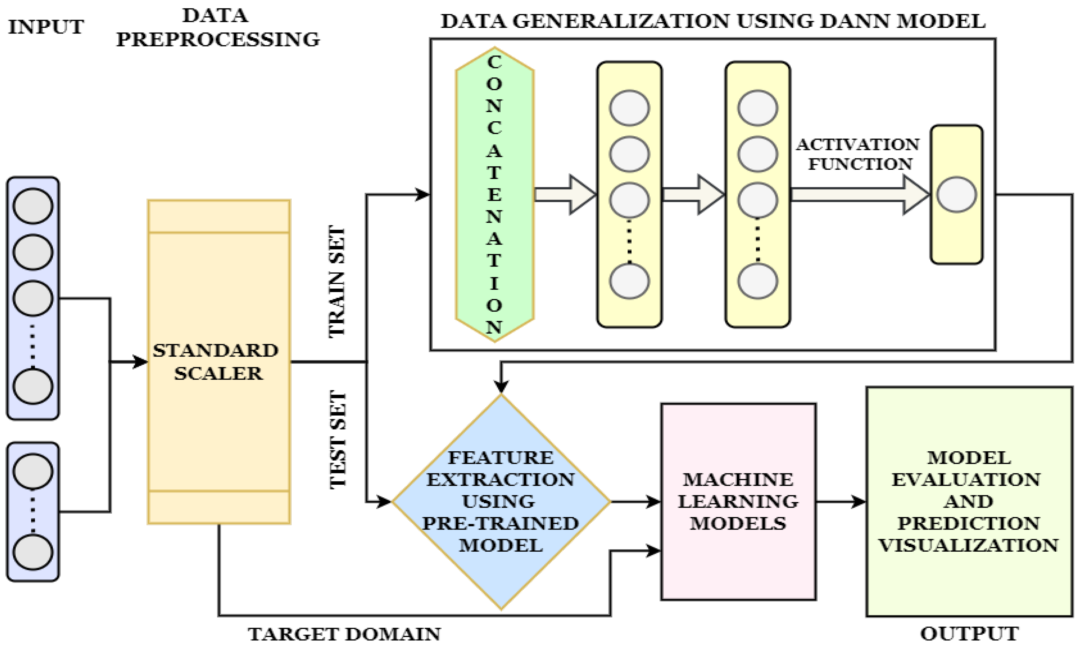
3. Proposed Methodology

According to the related work, ML and ensemble learning models struggle with limited samples and high variability. The supply chain management of the FMCG dataset from Bangladesh, described in Section 3.1, is analyzed for statistical and stationarity characteristics in Section 3.2. The data is then preprocessed and generalized using the DANN model, ensuring that the output data retains properties similar to the original dataset. A pre-trained model achieves demand prediction for products in the test set with state-of-the-art ML models, effectively implementing a transfer learning approach. The block diagram of the proposed methodology is shown in Figure 1. Section 3.3 covers data processing, while Section 3.4 describes the DANN model’s generalization process, ensuring the augmented data resemble the original data, as evidenced in the results section. Section 3.5 discusses various ML models used for analysis, with the testing dataset processed based on the DANN-augmented training input, demonstrating the implementation of transfer learning. The pipeline and flow of methodology can be seen from Algorithm 1; note that the step does not represent the subsection of the proposed methodology.

Algorithm 1 Pipeline of Proposed Methodology

1: Step 1: Analysis of the Dataset   2:     1.1 Load the dataset.   3:     1.2 Explore the dataset to understand its structure and characteristics.   4:     1.3 Identify any patterns, missing values, and outliers.   5:     1.4 Analyze the stationarity of the data using statistical tests (KPSS test).   6: Step 2: Dataset Preprocessing   7:     2.1 Handle missing values and outliers.   8:     2.2 Normalize or standardize the dataset.   9:     2.3 Split the dataset into training and testing sets. 10: Step 3: DANN Implementation on the Training Dataset 11:     3.1 Initialize the DANN model with feature extractor and domain discriminator. 12:     3.2 Train the DANN model on the training dataset. 13:     3.3 Minimize the mean squared error loss between predicted and actual values while adapting to domain shifts. 14: Step 4: Utilizing Training Dataset Weights 15:     4.1 Extract weights from the trained DANN model. 16:     4.2 Apply these weights to subsequent DANN layers. 17:     4.3 Use the generalized weights for implementation. 18: Step 5: Implement ML Models with Testing Set 19:     5.1 Input the scaled target domain into various ML models (Linear Regression, SVR, Decision Tree Regressor, Random Forest, XGBoost Regressor). 20:     5.2 Use the DANN-trained weights to enhance the predictions of these ML models, demonstrating transfer learning on test data. 21: Step 6: Calculate Performance of Models 22:     6.1 Evaluate the performance of each model on the test data. 23:     6.2 Calculate metrics such as Mean Absolute Error ($MAE$), Mean Squared Error ($MSE$), Root Mean Squared Error ($RMSE$), Mean Absolute Percentage Error ($MAPE$), and $R^{2}Score$ ($R^2$). 24:     6.3 Compare the performance of different models to identify the best-performing one.

3.1. Dataset Description

The research authors presented the SupplyGraph dataset [22], which included temporal and graphical data for 41 products. The researchers collected this dataset from FMCG companies operating in Bangladesh, explicitly emphasizing the temporal element. The 41 products in the dataset are grouped into five product groups, and then each group is further broken into smaller sub-groups. It is important to note that the dataset does not contain explicit product names; instead, product IDs issued to each group and subgroup are used to identify the products.

The collected dataset [22] spans from 1 January 2023, to 9 August 2023, and resulted in 221 entries. Researchers arranged every CSV file of this span, with 41 distinct columns indicating the corresponding Product IDs. There are eight CSV files, namely Delivery to Distributor, Factory Issue, Production, and Sales Order, each having two files of the respective count of units and weights. The sales order files provide information on overall product demand. It means that it shows distributor-requested amounts pending approval from the accounts department. On the other hand, Delivery to Distributors keeps track of products shipped by orders, significantly impacting business income. Factory Issue, on the other hand, refers to the total amount of goods shipped from production sites, along with distribution and storage warehouse shares. Production measures the amount of product produced while considering sales orders, client demand, vehicle fill rate, and urgency of delivery.

The product categorization system consists of five groups: A, S, P, M, and E, having subgroups which can be seen in Figure 2. Product group S has four distinct subgroups, including SOS, SOP, SO, and SE, having seven, one, four and three products, respectively. Product group P has three subgroups, including POV, POP, and POPF, encompassing four, six and one products. Product group A has five subgroups, including AT, ATN, ATWWP, ATPPCH, and ATPA, having one, two, two and one products, respectively. MAR, MASR, MAHS, MAPA, MAC, and MAP. Product group M has six subgroups, including MAR, MASR, MAHS, MAPA, MAC, and MAP, that consist of two, one, one, one, one and one products, respectively. Finally, product group E has an EEA subgroup with two products. The initial alphabet shows a group, whereas a further alphabet shows a sub-group of its respective product unit in a factory. For example, this is a product id ‘AT5X5K’ where A is a group and further alphabets like T show their subgroup, which can also be seen from Figure 2 as ‘AT’ subgroup, after which in product ID their unique ID is followed. So, similar for other subgroups is also to be considered. This structured classification helps efficiently organize and manage the diverse range of products within each group and subgroup used to identify the products.

3.2. Data Handling and Analysis

To optimize data organization and enable the adoption of our suggested methodology, the data are organized into 41 CSV files, each containing the temporal data for all eight attributes previously included in a different CSV file. To conduct this, the columns from eight CSV files were divided according to product, which resulted in the creation of 41 CSV files organized for each corresponding good. The dataset’s organization facilitates easy access and analysis, enabling researchers to successfully implement their suggested technique and obtain valuable information on supply chain dynamics and product performance using a transfer learning approach for forecasting.

Figure 3 shows a product’s maximum value range for eight features across 41 products. Some products have low or no values, so they are considered for dropping. Twelve products are dropped, resulting in 29 features. These products are considered in Figure 4, excluding the dropped products. Figure 4 shows the standard deviation of the products for all eight features, indicating the high variability in the dataset distribution.

To analyze non-stationarity in the data, we utilized the KPSS test, because it is particularly effective for detecting stationarity in the presence of a unit root. A unit root indicates that the time series is non-stationary, meaning its mean and variance can change over time, making it unpredictable and difficult to model. Given that our dataset is small and exhibits high variability, the KPSS test is especially useful. It checks for the null hypothesis of stationarity, providing a different perspective compared to tests like the Dickey–Fuller and Phillips–Perron tests, which test for the null hypothesis of a unit root (non-stationarity). This complementary approach helps ensure a more robust analysis of the data’s stationarity characteristics.

Non-Stationary Testing of the Dataset

A statistical test called the Kwiatkowski–Phillips–Schmidt–Shin (KPSS) test assesses if a set of time series data is stationary. When statistical parameters like mean, variance, and autocovariance do not change over time, a time series is said to be stationary. The purpose of the KPSS test is to identify that a given time series possesses non-stationarity, which is frequently indicated by having pattern breaks or is stationary around a stable trend. The KPSS test is implemented according to Equations (1) and (2). The null hypothesis suggests the data in a respective product ID are stationary, meaning their properties remain constant over time. The alternative hypothesis suggests the series is non-stationary, with mean, variance, or autocovariance changes. These hypotheses allow the statistical tests to assess the series’s stationarity, providing knowledge about its dynamics and patterns. Evaluate the nature of the dataset, the KPSS test is used here for the features in a dataset. This allows checking features’ stationary or non-stationary behavior as this dataset contains high variability.

$$y_t=\alpha +\beta t+{\epsilon }_t$$

(1)

$$p\text{-}\mathrm{value}={\displaystyle \frac{SSR}{{\sigma }^2}}$$

(2)

where $y_t$ is the time series data at time t, $\alpha$ is the intercept term, $\beta$ is the coefficient of the time trend, t is time and ${\epsilon }_t$ is the error term, p-value contains KPSS test value, ${\sigma }^2$ is the variance and $SSR$ is the sum of the square of residuals whose formula can be seen in Equation (3).

$$SSR=\sum _{t=1}^T{\widehat{\epsilon }}_t^2$$

(3)

where $SSR$ is the Sum of Squared Residuals, ${\widehat{\epsilon }}_t$ represents the residual (difference between the observed value and the predicted value) at time t, and T is the total number of observations in the time series.

To perform the KPSS test, the estimated regression model’s sum of squared residuals ($SSR$) is evaluated. Then, using variance and $SSR$ the p-values are computed and compared with critical values, based on the selected significance level. If the calculated test statistic is above the critical value, the null hypothesis of stationarity is rejected, hence offering evidence against stationarity around a deterministic trend. On the other hand, if the test statistic is less than the critical value, stationarity should be applied to keep the null hypothesis from being rejected. Here, the essential values used are taken as 0.05. All the results of the features in a single product are aggregated, and the value is noted in a KPSS result column in

Table 1. KPSS Results for all the selected Product ID.

Sr. No.	Product ID	Stationarity	KPSS Result (p-Value)	Sr. No.	Product ID	Stationarity	KPSS Result (p-Value)
1	AT5X5K	NS	0.0419	16	POV001L24P	NS	0.01
2	ATN01K24P	S	0.1	17	POV002L09P	S	0.1
3	ATN02K12P	S	0.1	18	POV005L04P	S	0.1
4	ATWWP001K24P	NS	0.046	19	POV500M24P	S	0.0993
5	ATWWP002K12P	S	0.1	20	SE200G24P	NS	0.01
6	MAR01K24P	S	0.1	21	SE500G24P	NS	0.019
7	MAR02K12P	NS	0.049	22	SOP001L12P	NS	0.025
8	MASR025K	S	0.1	23	SOS001L12P	NS	0.01
9	POP001L12P.1	S	0.1	24	SOS002L09P	NS	0.022
10	POP001L12P	S	0.089	25	SOS003L04P	NS	0.0254
11	POP002L09P	S	0.074	26	SOS005L04P	NS	0.01
12	POP005L04P	NS	0.048	27	SOS008L02P	NS	0.01
13	POP500M24P	S	0.826	28	SOS250M48P	Non-Stationary	0.025
14	POPF01L12P	NS	0.036	29	SOS500M24P	NS	0.05
15	MAHS025K	NS	0.029

NS (Nonstationary); S (Stationary).

. The table only consists of the selected features.

3.3. Data Preprocessing

The dataset is small, with 221 rows, emphasizing the need to consider standard deviation and limited data analysis. Processing such a dataset is challenging; our proposed methodology addresses this and aims to improve predictions. As discussed in Section 3.2, some products have low or no values; they are considered for dropping, which can be analysed and seen from Figure 3. Twelve products are dropped, resulting in 29 products. The standard scaling on all features individually is performed. The sales order feature is used as the target variable. The random division of the dataset into training and test sets ensures adequate variability for assessment. The selected dataset, discussed in Section 3.1 and Section 3.2, is split into training (62%) and test (38%) sets, with 18 CSV files for training and 11 for testing, based on observed variability and characteristics.

Standard scaling is essential for practical model training and generalization in selected datasets with limited samples and high variability, particularly using methods such as DANN. It fits feature distributions across domains and reduces the effect of variability by normalizing features to a constant mean and standard deviation. By reducing domain differences and promoting meaningful representation learning, this alignment helps the model perform better on unseen data. Ensuring that the DANN model’s output data maintain characteristics from the original dataset, standard scaling helps provide practical model training and accurate generalization to new data. Every data point contributes when working with small datasets, and standard scaling improves the utility of each observation made during training. This enhances the performance of machine learning models and the quality of augmented or generalized data. The formula for standard scaling can be seen in Equation (4).

$$Z={\displaystyle \frac{x-\mu }{\sigma }}$$

(4)

where $\mu$ is the mean (average) of the data set, x is the individual data point being standardized, $\sigma$ is the standard deviation of the data set, which measures the amount of variation or dispersion of the data points from the mean and the Z is a z-score, which indicates how many standard deviations a data point x is from the mean $\mu$.

3.4. Domain Adversarial Neural Network

A DANN is a type of neural network architecture developed to address machine learning problems related to domain adaptation. It aims to gather invariant data representations across different domains, enabling efficient knowledge transfer from a distributed source domain to another. For this, DANN utilizes a domain discriminator and a feature extractor. The feature extractor can extract valuable features by manipulating the domain discriminator to perceive no difference between the source and target domains. This is made achievable through a crucial component named the gradient reversal layer, which encourages the feature extractor to learn domain-invariant representations by reversing the gradients during back-propagation, which is achieved by minimizing the Mean Squared Error ($MSE$) loss in this proposed scenario.

There are two layers in this feature extractor of the model. The initial layer comprises 64 neurons, and the following layer shall consist of 32 neurons. ReLU activation functions are utilized in both layers to input the non-linearity and understand the model better. The model uses an adversarial training framework to minimize the mean squared error loss between the predicted and actual target values throughout training. A single neuron with a linear activation function to not complicate, which generates regression predictions, is often referred to as the output layer of the DANN model. The augmented data from all source domains are concatenated into a single array along the columns axis, pooling domain knowledge from all source domains after the DANN model is trained for each source domain, and the target training data are assisted using the weights of trained model for the proper understanding. The scaled target domain is directly inputted into the different ML models to predict the output demand of the unseen product.

The mathematical model of the hidden layer and output layer of the DANN model for data generalization can be seen from Equations (5)–(7).

$$H_a=f_{ReLU}(W_a.X+B_a)$$

(5)

$$H_b=f_{ReLU}(W_b.H_a+B_b)$$

(6)

$$Y_{generalized}=f_{Linear}(W_{output}.H_b+B_{output})$$

(7)

where, $H_a$, $H_b$ are the hidden layers, $W_a$, $W_b$, and $W_{output}$ are the weights associated with the respective layers. $B_a$, $B_b$, and $B_{output}$ are the bias associated with the respective layers. $Y_{generalized}$ is the generalized output of the DANN model.

In the output layer, linear activation maintains the direct correlation between the final output and the learned features, improving understanding and accurately demonstrating the model’s generalization capabilities. Predicting continuous values in regression problems is especially helpful. Additionally, while dealing with the saturation problem that comes with nonlinear activation functions, linear activation guarantees steady, fast, and practical training; however, for learning complex representations of the data in a DANN model, the feature extractor in a DANN model via nonlinear ReLU activation function in hidden layers; formula for ReLU and linear activation function can be found from the Equation (8) and Equation (9), respectively. For DANN models to be successful in domain adaptation tasks, the model must have this non-linearity to generalize well across domains and adjust to changes in the domain. Therefore, nonlinear activation functions like ReLU allow the model to learn complicated patterns and adapt to domain shifts successfully. In contrast, linear activation in the output layer can benefit regression tasks.

$$f_{ReLU}=max(0,x)$$

(8)

$$f_{Linear}=x$$

(9)

where $f_{ReLU}$ and $f_{Linear}$ are the ReLU and Linear activation functions for the associated value of x.

The study applied DANN on training datasets for generalization due to DANNs’ effectiveness in domain adaptation, minimizing domain-specific biases, and improving predictive accuracy without the complexity of LSTM and GRU. The training data were used to assess the DANN model’s augmented ability. The focus was on the practical application of DANN in optimizing supply chain operations, leveraging its unique capabilities to address domain shifts and enhance generalization. Using other adversarial models would increase complexity and cost. This DANN model will be used and embedded with ML models to predict the products in test data that were not considered in train data.

3.5. Machine Learning Models

The transfer learning approach for newer domains is tested on testing data using the generalized dataset weight-based assisted inputs on different ML models.

3.5.1. Linear Regression Model

Linear regression is a common technique used in machine learning to model the relationship between independent and dependent variables. It is typically used in forecasting scenarios and assumes that the variables have a linear relationship with each other [31]. Linear regression aims to identify the best coefficients that minimize the difference between the actual and expected values. Before using linear regression, it is essential to validate its assumptions, which include linearity, uniformity, error independence, and residual normality. Despite its simplicity, linear regression is a powerful statistical tool that provides interpretable results and a helpful baseline for complex model comparisons. Additionally, it offers testing instruments for evaluating model assumptions.

3.5.2. Support Vector Regressor Model

The Support Vector Regressor (SVR) [32] is a regression approach to predict continuous results in complex or nonlinear relationships between target variables and predictors. The hyperplane that maximizes the margin between data points and the hyperplane that best fits the training data is determined in a high-dimensional space. Support vectors, a subset of training data, are used to determine this hyperplane. SVR controls a margin of error, defined by an epsilon parameter, and minimizes the error between the expected and actual values. One of the advantages of SVR is that it is sensitive to outliers and capable of handling high-dimensional data. SVR includes different kernel functions such as radial, polynomial, and linear to capture various types of relationships between the variables.

3.5.3. Decision Tree Regressor Model

Decision Tree Regressor (DTR) is a regression technique that models the relationship between predictors and a continuous target variable using a tree-like structure. This model is important because it divides the feature space sequentially into smaller areas, each corresponding to a decision node in the tree. This approach uses a criterion, like reducing the variance of the target variable inside each partition, to choose the feature and split point that best divides the data. Decision trees are simple and easy to understand, making them helpful in figuring out the underlying patterns in the data [33].

Model efficiency and overfitting are reduced by parameters such as the criteria, max depth, min samples split, min samples leaf, and max features, which control the minimum number of samples needed for node splitting, leaf formation, and the maximum number of features considered for each split. To optimize these parameters and achieve a balance between model complexity and generalization ability, hyperparameter tuning becomes essential [34]. Decision Tree Regressor model can be operated optimally on unobserved data by fine-tuning the parameters. This will allow the model to adjust its behavior to the unique features of the dataset and produce the best possible predicted performance. Trimming, ensemble approaches, and limiting tree depth are commonly employed to overcome an overfitting problem.

3.5.4. Random Forest Regressor Model

The Random Forest Regressor model is a very effective method for producing accurate predictions for regression tasks. This is due to its ability to combine multiple decision trees to create dependable and precise predictions. The model also promotes diversity and reduces overfitting by constructing each decision tree using a random subset of the training data and a random subset of features. It is essential to adjust the model’s hyperparameters to achieve optimal performance. Parameters such as the number of trees ($n_{estimators}$) and the maximum depth of each tree ($ma{x}_{depth}$) play a crucial role in balancing the variance and bias of the model. Other parameters such as $mi{n}_{samples\_split}$, $mi{n}_{samples\_leaf}$, and $ma{x}_{features}$ also contribute to the performance of the model by controlling node splitting, leaf formation, and the number of features taken into account for each split. Fine-tuning these parameters using methods like grid search or random search can help the model adapt to the unique features of the dataset, maximizing predicted accuracy while limiting overfitting [34].

3.5.5. Extreme Gradient Boost XGBoost Regressor Model

An ensemble learning approach, the XGBoost Regressor model is used for regression problems due to its exceptional performance. It gradually builds an ensemble of weak decision trees, using regularization techniques to keep the model simple and optimizing a differentiable loss function to minimize errors at each stage. Optimizing the model’s hyperparameters is crucial for the best possible prediction performance. Two important parameters are the number of boosting rounds ($n_{estimators}$), which determines the number of weak learners in the ensemble, and the learning rate, which controls the step size during gradient descent.

3.6. Performance Parameters of Model

When evaluating the performance of an ML and DANN model, various metrics such as Mean Squared Error ($MSE$), Mean Absolute Error ($MAE$), $R^2$ Score, and Root Mean Squared Error ($RMSE$) can be used. $MSE$ measures the average squared difference between the actual and predicted values, while $MAE$ computes the average absolute difference between them. $R^2$ Score quantifies the proportion of the dependent variable’s variance that can be predicted from the variance of the independent variables, and a higher value indicates better model performance. $RMSE$ is the square root of the $MSE$ and measures the average magnitude of the errors in the same units as the target variable, making it easier to interpret. The formula for $MSE$, $RMSE$, $MAE$ and $R^2$ Score can be seen in Equations (10)–(13), respectively.

$$MSE={\displaystyle \frac{1}{n}}\sum _{i=1}^n{(y_i-{\widehat{y}}_i)}^2$$

(10)

$$RMSE=\sqrt{{\displaystyle \frac{1}{n}}\sum _{i=1}^n{(y_i-{\widehat{y}}_i)}^2}$$

(11)

$$MAE={\displaystyle \frac{1}{n}}\sum _{i=1}^n|y_i-{\widehat{y}}_i|$$

(12)

$$R^2=1-{\displaystyle \frac{{\sum }_{i=1}^n{(y_i-{\widehat{y}}_i)}^2}{{\sum }_{i=1}^n{(y_i-\overline{y})}^2}}$$

(13)

where n represents the number of samples, $y_i$ denotes the actual target value of the ith sample, ${\widehat{y}}_i$ represents the predicted target value of the ith sample, and $\overline{y}$ represents the mean of the actual target values.

4. Results and Discussion

The study focuses on supply chain management and predictive modeling, specifically examining the effectiveness of DANN with limited sample and high-variability datasets. It evaluates the performance of machine learning models like Linear Regression, RF, DTR, XGBoost and SVR when enhanced with DANN-trained weights for demand forecasting in the fast-moving consumer goods sector. Temporal data from the SupplyGraph dataset are integrated to improve demand prediction accuracy. DANN is trained and evaluated on the training data to assess its augmenting and generalizing capabilities. The hypotheses suggest that DANN enhances the generalization capabilities of these models, resulting in superior predictive performance in supply chain applications. Section 4.1 discusses the DANN model’s ability, Section 4.2 provides a comparative analysis of the ML models’ performance, and Section 4.3 discusses the implications of this study.

4.1. Results of DANN Model for Data Generalization

The DANN model framework utilizes products in the training dataset that can be seen in

Table 2. Performance evaluation of the DANN model on train set for data generalization and training weight construction.

Sr. No.	Product ID	$\mathit{M}\mathit{S}\mathit{E}$	$\mathit{R}\mathit{M}\mathit{S}\mathit{E}$	${\mathit{R}}^2$ Score	$\mathit{M}\mathit{A}\mathit{E}$	$\mathit{M}\mathit{A}\mathit{P}\mathit{E}$
1	AT5X5K	0.014	0.118	0.985	0.078	0.28
2	ATN01K24P	0.01	0.102	0.989	0.077	0.24
3	ATN02K12P	0.027	0.164	0.972	0.096	0.72
4	MAR01K24P	0.011	0.104	0.988	0.082	0.34
5	MAR02K12P	0.012	0.109	0.987	0.076	0.24
6	POP001L12P.1	0.008	0.089	0.991	0.06	0.44
7	POP001L12P	0.022	0.148	0.977	0.084	0.58
8	POP002L09P	0.016	0.126	0.983	0.094	0.345
9	POPF01L12P	0.012	0.109	0.987	0.074	0.335
10	POV001L24P	0.028	0.167	0.971	0.107	0.32
11	SE200G24P	0.015	0.122	0.984	0.08	0.265
12	SE500G24P	0.015	0.122	0.984	0.089	0.328
13	SOP001L12P	0.0107	0.103	0.989	0.085	0.226
14	SOS001L12P	0.008	0.089	0.991	0.073	0.38
15	SOS008L02P	0.011	0.105	0.988	0.078	0.24
16	SOS002L09P	0.04	0.197	0.956	0.13	0.49
17	SOS003L04P	0.017	0.13	0.982	0.102	0.38
18	SOS005L04P	0.008	0.089	0.991	0.073	0.18

to learn the underlying patterns in the sales order data. Through the training process, the model retrieves weights that will be further used to optimize forecasting performance. In Figure 5, the effectiveness of the DANN framework in generalizing the sales order data for a specific product ID, SOS001L12P, is visualized. Notably, this product exhibits a higher standard deviation of sales orders than others, as evident from Figure 4.

The performance of the DANN model in generalizing the data is further assessed through various evaluation metrics presented in Table 2. These metrics include $MSE$, $MAPE$, $RMSE$, $MAE$ and $R^2$ Score. Lower $MSE$, $MAPE$, and $RMSE$ values indicate that the model’s predictions closely match the actual sales order values. In contrast, a higher R² Score signifies a better fit of the model to the data, capturing a more significant proportion of the variance in sales orders. The results in Table 2 demonstrate that the DANN model has performed well, as indicated by the lower values of $MSE$, $MAPE$, and $RMSE$, along with a higher R² Score. These metrics collectively indicate the model’s ability to effectively generalize the sales order data while maintaining the original behavior, as shown in Figure 5. Thus, the DANN framework successfully captures the variability in sales orders, facilitating accurate predictions and maintaining the originality for product SOS001L12P. After analyzing the results, it can be seen that the DANN model is better for product SOS001L12P and all the products in the train set. The evaluation metrics in Table 2 indicate that the model has performed well, demonstrating its ability to generalize sales order data across all products.

4.2. Comparative Study of Outcomes of Various Machine Learning Models

It has been observed that the DANN framework performs better for generalizing and predicting the sales order of products with a sufficient standard deviation. Even for products without historical data, the DANN model can accurately predict sales orders by using the patterns it learned from the data of other products in the train set. However, in some cases, using Deep Learning (DL) models can enhance the complexity and processing demands. Although DL models can offer competitive performance in predicting sales orders for unknown FMCG products, they may not always be practical due to their high processing demands. Incorporating ML models for testing frameworks can be a better alternative to achieve better results in sales order prediction.

The ML model is trained on the dataset and then applied to the testing data, which may contain unknown or distinct products from the training set through transfer learning. The DANN model and the trained weights are utilized in this approach for feature extraction. Using a more straightforward ML learning framework, businesses can generate precise sales estimates for unknown products without incurring the expenses associated with DL architectures. Companies must be able to adjust and generalize when predicting sales for various newer product portfolios. Even though these models are more straightforward, they can still provide accurate predictions, especially when trained with enough data and relevant features.

Based on the transfer learning approach, the DANN model extracts features using the weights from the train set. These extracted features are then further processed using various ML models incorporating a standard scaled target domain to make predictions. Several ML models, including Linear Regression, Support Vector Regressor, Decision Tree Regressor, Random Forest Regressor, and XGB Regressor, are used, and their evaluation capabilities are analyzed for forecasting sales in a limited and highly variable dataset.

Table 3. Performance evaluation of ML models [Linear Regression, SVR (Linear Kernel), SVR (RBF Kernel) and XGBoost Regressor] on the test set for sales order prediction.

Model	Product ID	Performance Metrics
		$\mathit{M}\mathit{S}\mathit{E}$	$\mathit{R}\mathit{M}\mathit{S}\mathit{E}$	${\mathit{R}}^{\mathit{2}}$ Score	$\mathit{M}\mathit{A}\mathit{E}$	$\mathit{M}\mathit{A}\mathit{P}\mathit{E}$
Linear Regression	ATWWP001K24P	0.014	0.121	0.985	0.085	0.526
	ATWWP002K12P	0.011	0.109	0.988	0.075	0.572
	MAHS025K	0.012	0.11	0.987	0.072	0.253
	MASR025K	0.036	0.18	0.963	0.143	0.41
	POP005L04P	0.039	0.198	0.96	0.147	0.57
	POP500M24P	0.125	0.353	0.874	0.25	0.74
	POV002L09P	0.042	0.205	0.957	0.161	0.72
	POV005L04P	0.03	0.175	0.969	0.136	0.613
	POV500M24P	0.025	0.16	0.974	0.124	0.6
	SOS250M48P	0.06	0.245	0.939	0.175	0.523
	SOS500M24P	0.081	0.284	0.918	0.223	0.575
SVR (Linear kernel)	ATWWP001K24P	0.018	0.136	0.98	0.106	0.56
	ATWWP002K12P	0.015	0.12	0.984	0.085	0.58
	MAHS025K	0.012	0.11	0.987	0.074	0.254
	MASR025K	0.038	0.19	0.969	0.14	0.4
	POP005L04P	0.04	0.2	0.959	0.147	0.52
	POP500M24P	0.127	0.35	0.87	0.25	0.81
	POV002L09P	0.045	0.21	0.954	0.163	0.68
	POV005L04P	0.032	0.17	0.967	0.135	0.54
	POV500M24P	0.026	0.16	0.973	0.127	0.65
	SOS250M48P	0.061	0.24	0.938	0.16	0.55
	SOS500M24P	0.082	0.28	0.917	0.22	0.57
SVR (RBF kernel)	ATWWP001K24P	0.023	0.152	0.976	0.11	0.69
	ATWWP002K12P	0.112	0.335	0.887	0.11	0.55
	MAHS025K	0.053	0.23	0.966	0.107	0.26
	MASR025K	0.142	0.377	0.857	0.14	0.34
	POP005L04P	0.078	0.28	0.921	0.131	0.5
	POP500M24P	0.06	0.26	0.932	0.17	0.76
	POV002L09P	0.034	0.18	0.965	0.11	0.31
	POV005L04P	0.031	0.17	0.968	0.1	0.34
	POV500M24P	0.029	0.17	0.97	0.1	0.64
	SOS250M48P	0.063	0.25	0.936	0.142	0.39
	SOS500M24P	0.046	0.214	0.953	0.14	0.49
XGBoost Regressor	ATWWP001K24P	1.17 × ${10}^{-6}$	0.001	0.999	7.5 × ${10}^{-4}$	0.003
	ATWWP002K12P	9.31 × ${10}^{-7}$	9.6 × ${10}^{-4}$	0.999	5.8 × ${10}^{-4}$	0.0031
	MAHS025K	5.65 × ${10}^{-7}$	7.5 × ${10}^{-4}$	0.999	4.8 × ${10}^{-4}$	0.0025
	MASR025K	1.14 × ${10}^{-7}$	0.001	0.999	7.32 × ${10}^{-4}$	0.0059
	POP005L04P	9.17 × ${10}^{-7}$	9.5 × ${10}^{-4}$	0.999	6.4 × ${10}^{-4}$	0.0039
	POP500M24P	1.25 × ${10}^{-6}$	0.0011	0.999	8 × ${10}^{-4}$	0.017
	POV002L09P	9.55 × ${10}^{-7}$	9.7 × ${10}^{-4}$	0.999	7.1 × ${10}^{-4}$	0.0028
	POV005L04P	1.59 × ${10}^{-6}$	1.26 × ${10}^{-3}$	0.999	8.7 × ${10}^{-4}$	0.0048
	POV500M24P	1.36 × ${10}^{-6}$	0.0011	0.999	8.4 × ${10}^{-4}$	0.0044
	SOS250M48P	1.1 × ${10}^{-6}$	0.001	0.999	7 × ${10}^{-4}$	0.0027
	SOS500M24P	9 × ${10}^{-7}$	9.5 × ${10}^{-4}$	0.999	6.8 × ${10}^{-4}$	0.0036

displays the performance metrics values for Linear Regression, SVR, and XGB Regressor to predict sales orders. Figure 6 showcases the graphical relationship between these ML models’ expected and actual sales order values. This graph includes the required, ideal predictions and the experimentally predicted data distribution for different ML models, making it easier to compare them through visualization.

The Linear Regression model performed well in predicting the dataset. However, the variation in data does not impact the prediction models. For the ATWWP001K24P product, the linear regression and SVR with a linear kernel model prediction graphically can be seen in Figure 6a and Figure 6b, respectively. The linear regression and SVR performance metrics with a linear kernel show comparatively better results, though they still need to reduce and enhance the parameters. Using an SVR with an RBF kernel, the prediction does not show a better result than the Linear Regression and SVR with a linear kernel. Prediction using an SVR with an RBF kernel model can be seen in Figure 6c. The performance evaluation for the polynomial kernel was also analyzed, but it showed poor results. This ATWWP001K24P product shows R² Score of 0.89; it does not perform relatively better for other models. That is why the polynomial kernel is dropped to consider for comparison. From this graph and analysis for all the products, it is found that there are comparatively and sufficiently high biases impacting the forecasting performance metrics. RMSE can be reduced further by using a different ML model with a hierarchical and better knowledge-extracting and analysis model using DTR and ensemble learning approaches.

Using a DTR and RF regressor model for prediction, the values of performance parameters can be seen in

Table 4. Performance evaluation of DTR and RF models on test set for sales order prediction for the best-tuned hyperparameters.

Model	Product ID	Best Hyperparameters 1	Performance Metrics
			$\mathit{M}\mathit{S}\mathit{E}$	$\mathit{R}\mathit{M}\mathit{S}\mathit{E}$	${\mathit{R}}^{\mathit{2}}$ Score	$\mathit{M}\mathit{A}\mathit{E}$	$\mathit{M}\mathit{A}\mathit{P}\mathit{E}$
DTR	ATWWP001K24P	[8; 2; 4]	0.011	0.108	0.988	0.048	0.19
	ATWWP002K12P	[7; 3; 4]	0.014	0.12	0.985	0.045	0.283
	MAHS025K	[8; 1; 6]	0.005	0.076	0.994	0.032	0.118
	MASR025K	[5; 1; 2]	0.015	0.123	0.984	0.087	0.55
	POP005L04P	[7; 1; 3]	0.006	0.079	0.993	0.044	0.395
	POP500M24P	[6; 3; 6]	0.04	0.204	0.958	0.132	0.83
	POV002L09P	[6; 2; 4]	0.016	0.129	0.983	0.094	0.59
	POV005L04P	[6; 4; 4]	0.021	0.147	0.978	0.088	0.386
	POV500M24P	[6; 2; 3]	0.008	0.092	0.991	0.067	0.29
	SOS250M48P	[6; 3; 4]	0.025	0.16	0.974	0.079	0.42
	SOS500M24P	[5; 3; 5]	0.063	0.252	0.936	0.171	0.81
RF	ATWWP001K24P	[8; 1; 2; 100]	0.005	0.072	0.994	0.03	0.13
	ATWWP002K12P	[5; 2; 2; 100]	0.0135	0.116	0.986	0.049	0.29
	MAHS025K	[8; 1; 4; 100]	0.004	0.07	0.995	0.034	0.12
	MASR025K	[8; 1; 2; 300]	0.006	0.083	0.993	0.04	0.27
	POP005L04P	[8; 1; 5; 100]	0.015	0.12	0.984	0.069	0.42
	POP500M24P	[8; 1; 3; 100]	0.023	0.153	0.976	0.108	0.69
	POV002L09P	[8; 1; 3; 100]	0.01	0.1	0.989	0.071	0.43
	POV005L04P	[7; 1; 2; 100]	0.005	0.076	0.994	0.054	0.21
	POV500M24P	[8; 1; 3; 300]	0.004	0.069	0.995	0.051	0.19
	SOS250M48P	[7; 1; 3; 100]	0.011	0.107	0.988	0.057	0.27
	SOS500M24P	[6; 2; 5; 100]	0.038	0.195	0.961	0.133	0.77

¹ [max_depth;min_sample_leaf;min_sample_split;n_estimators].

. DTR and RF perform relatively better than all the other models discussed before (SVR, Linear Regression) except the XGB Regressor model. The best possible parameters associated with the best prediction performance results can be found in Table 4. The critical parameters like maximum depth (max_depth) are looped from 1 to 10, minimum samples leaf nodes looped from 1 to 5, and minimum nodes samples split are looped from 1 to 6, and the best possible combination is obtained for DTR. The parameters in RF are the same as DTR with an additional number of estimator ($n\_estimator$) parameters looped from 100 to 300 with a step size of 100. For the ATWWP001K24P product, both models show better results and can be visually analyzed from Figure 7a. In this figure, the black line shows the ideal prediction of the model. The data point’s residual formula can be seen from Equation (14). The residuals are the differences between the predicted values and the actual values. A residual is essentially the error of the model for each data point. For this product the $RMSE$ is 0.072 and $MAPE$ of 13% for the RF model whereas for DTR, $RMSE$ is 0.108 and $MAPE$ of 19%; which shows that the RF model has worked better than others with an average of 25% and DTR with an average of 12% and in comparison to DTR and RF models the RF has performed approximately 20% more than DTR.

$${ϵ}_i=y_i-{\widehat{y}}_i$$

(14)

where the ${ϵ}_i$ is the residual for the data point, $y_i$ is the observed value (actual value) for the data point, and ${\widehat{y}}_i$ is the predicted value for the data point as estimated by the regression model.

In our study, after experimentation, the RF regression model emerged as a better performer than others except for the XGBoost Regressor model, as evidenced by the uniform distribution of residuals observed in the residual vs. actual values plot in Figure 7b. In this figure, the black line shows the reference line for the distribution of residual. This uniform distribution signifies the model’s ability to accurately capture the underlying patterns within the data, leading to reliable predictions across the entire range of actual values. The RF model, trained using ensemble learning techniques and decision trees, exhibits robustness against overfitting and high predictive accuracy. Its hyperparameter tuning enhances its reliability in real-world applications. The model’s uniform residuals show minimal systematic errors or biases, making it a reliable tool for regression tasks across various domains. The hyperparameters are chosen based on experiments that minimize Mean Squared Error ($MSE$) within the specified ranges discussed in the respective models in this subsection. The tuned best hyperparameters can be seen from Table 4.

XGBoost Regression model performs better than all the other models as it is an advanced ML model incorporating a gradient boosting approach to build decision trees sequentially, learning from previous errors, thereby continuously improving performance by focusing on harder-to-predict data points. L1 (Lasso) and L2 (Ridge) regularization terms are used in XGBoost in its objective function to prevent overfitting and improve generalization performance, penalizing complex models and controlling tree complexity. The analyses of the result for XGBoost can be seen in Figure 6d and Table 3. Values of $MSE$ are in the range of ${10}^{-6}$ and ${10}^{-7}$ showing significantly better outcomes. For individuals, Lasso and Ridge with an alpha of 0.1, were evaluated, and it was found that Lasso worked relatively similarly to the linear regression, whereas Ridge performed poorer. XGBoost with a 0.3 learning rate, six as maximum depth, and 100 n_estimators, the model performs much better than we obtain from this experimented study. That is why hyperparameter tuning is ignored here. For the XGBoost algorithm, the ATWWP001K24P product shows the $RMSE$ of 0.001 and 0.3% of $MAPE$, which performs significantly better than DTR and RF models as their values of $MSE$ are in the range of ${10}^{-6}$ and ${10}^{-7}$.

4.3. Sales Prediction for Supply Chain Optimization

Forecasting sales are essential to supply chain management and planning process optimization [35]. Businesses can better handle resources and consider changes in demand by utilizing machine learning (ML) models and transfer learning techniques to estimate future sales trends for an unknown product based on historical knowledge [9,36]. This method increases the effectiveness of developing models and deployment by utilizing knowledge gained from earlier products through a transfer approach. Precise sales forecasts for various items, based on the delivery to the distributor, factory issue, and production unit, can be helpful. These features are essential to analyze FMCG products’ production and dispatch capability. Complex patterns and relationships in sales data are captured by ML algorithms like XGBoost, allowing for more accurate forecasts. Enhancing prediction capabilities is another benefit of using low-complexity ML models according to the performance results of the ML models discussed in Section 4.3. Integrating transfer learning, machine learning, and sales prediction creates a practical supply chain planning and optimization set that boosts competitiveness and efficiency in FMCG firms’ rapidly changing business environment nowadays [37].

5. Conclusions

In supply chain optimization, it is essential to understand the sales or demand for products according to the production and distribution system’s capabilities. For rapidly changing and growing FMCG companies, this sales prediction can help reduce the loss and enhance the profit, practicing sustainability, etc. In a scenario where the amount of data is less, the data size is small, and there is sufficiently high variability, it becomes too difficult to predict such an input condition using traditional ML models. A framework based on the Domain Adversarial Neural Network is proposed and utilized to train the data. It generalizes the data features and predicts the training sales order values. The simplicity of the model is maintained to maintain low complexity. This generalized feature has maintained its originality, confirmed through the visualization, and metrics like RMSE also show that it has retained its originality.

Further, this DANN model and the pre-trained weights are used for feature extraction of the features of an unknown product that are included in a test set. This model generalizes the features, whereas the target standard scaled data are directly inputted to the ML models. The ML models are used and analyzed to predict the sales order values. It was found that the Linear Regression and Support Vector Regressor with a Linear kernel performs better than the SVR with RBF and polynomial kernel, Lasso, and Rdige. Meanwhile, models like Decision Tree Regressor and Random Forest Regressor are tuned, and the best hyperparameters are obtained, but this model shows the best accuracy among the inputted parameters list. Random Forest performed better than Decision Tree and other models except for XGBoost Regressor. XGBoost Regressor has performed exceptionally better overall due to its gradient boosting capabilities, regularization techniques inclusion, and model complexity, allowing the model to predict well. In such a way, a transfer learning framework is implemented to forecast demand for supply chain optimization. This suggests that the DANN framework can be applied to similar datasets with different products and still produce accurate predictions. The success of the DANN model and ML-based transfer learning approach in this study highlights its potential as a valuable tool for forecasting sales orders and aiding business decision-making processes.

Further, this model can improved by using different deep neural network models. This model further can be implemented in an industry-based dataset for demand prediction. In this area, there is a need to collect more data and make them available for research. In the future, this methodology will be implemented across different datasets and application areas. The data characteristics and insights derived from this study can be extended to other domains for the prediction of required targets, enhancing the versatility and impact of the research.

References

1. McCarthy, T.M.; Golicic, S.L. Implementing collaborative forecasting to improve supply chain performance. Int. J. Phys. Distrib. Logist. Manag. 2002, 32, 431–454. [Google Scholar] [CrossRef]
2. Bourland, K.E.; Powell, S.G.; Pyke, D.F. Exploiting timely demand information to reduce inventories. Eur. J. Oper. Res. 1996, 92, 239–253. [Google Scholar] [CrossRef]
3. Tadayonrad, Y.; Ndiaye, A.B. A new key performance indicator model for demand forecasting in inventory management considering supply chain reliability and seasonality. Supply Chain Anal. 2023, 3, 100026. [Google Scholar] [CrossRef]
4. Arunachalam, D.; Kumar, N.; Kawalek, J.P. Understanding big data analytics capabilities in supply chain management: Unravelling the issues, challenges and implications for practice. Transp. Res. Part E Logist. Transp. Rev. 2018, 114, 416–436. [Google Scholar] [CrossRef]
5. L’heureux, A.; Grolinger, K.; Elyamany, H.F.; Capretz, M.A. Machine learning with big data: Challenges and approaches. IEEE Access 2017, 5, 7776–7797. [Google Scholar] [CrossRef]
6. Zhu, L.; Spachos, P.; Pensini, E.; Plataniotis, K.N. Deep learning and machine vision for food processing: A survey. Curr. Res. Food Sci. 2021, 4, 233–249. [Google Scholar] [CrossRef]
7. Al-Sahaf, H.; Bi, Y.; Chen, Q.; Lensen, A.; Mei, Y.; Sun, Y.; Tran, B.; Xue, B.; Zhang, M. A survey on evolutionary machine learning. J. R. Soc. N. Z. 2019, 49, 205–228. [Google Scholar] [CrossRef]
8. Zhou, L.; Zhang, C.; Liu, F.; Qiu, Z.; He, Y. Application of deep learning in food: A review. Compr. Rev. Food Sci. Food Saf. 2019, 18, 1793–1811. [Google Scholar] [CrossRef]
9. Bertolini, M.; Mezzogori, D.; Neroni, M.; Zammori, F. Machine Learning for industrial applications: A comprehensive literature review. Expert Syst. Appl. 2021, 175, 114820. [Google Scholar] [CrossRef]
10. Hu, H.; Xu, J.; Liu, M.; Lim, M.K. Vaccine supply chain management: An intelligent system utilizing blockchain, IoT and machine learning. J. Bus. Res. 2023, 156, 113480. [Google Scholar] [CrossRef]
11. Guo, H.; Zou, T. Cross-border e-commerce platform logistics and supply chain network optimization based on deep learning. Mob. Inf. Syst. 2022, 2022, 2203322. [Google Scholar] [CrossRef]
12. Kaya, S.K.; Yildirim, Ö. A prediction model for automobile sales in Turkey using deep neural networks. Endüstri Mühendisliği 2020, 31, 57–74. [Google Scholar]
13. Giri, C.; Chen, Y. Deep learning for demand forecasting in the fashion and apparel retail industry. Forecasting 2022, 4, 565–581. [Google Scholar] [CrossRef]
14. Kilimci, Z.H.; Akyuz, A.O.; Uysal, M.; Akyokus, S.; Uysal, M.O.; Atak Bulbul, B.; Ekmis, M.A. An improved demand forecasting model using deep learning approach and proposed decision integration strategy for supply chain. Complexity 2019, 2019, 9067367. [Google Scholar] [CrossRef]
15. Chien, C.F.; Lin, Y.S.; Lin, S.K. Deep reinforcement learning for selecting demand forecast models to empower Industry 3.5 and an empirical study for a semiconductor component distributor. Int. J. Prod. Res. 2020, 58, 2784–2804. [Google Scholar] [CrossRef]
16. Qi, M.; Shi, Y.; Qi, Y.; Ma, C.; Yuan, R.; Wu, D.; Shen, Z.J. A practical end-to-end inventory management model with deep learning. Manag. Sci. 2023, 69, 759–773. [Google Scholar] [CrossRef]
17. Amellal, I.; Amellal, A.; Seghiouer, H.; Ech-Charrat, M. An integrated approach for modern supply chain management: Utilizing advanced machine learning models for sentiment analysis, demand forecasting, and probabilistic price prediction. Decis. Sci. Lett. 2024, 13, 237–248. [Google Scholar] [CrossRef]
18. Alshurideh, M.T.; Hamadneh, S.; Alzoubi, H.M.; Al Kurdi, B.; Nuseir, M.T.; Al Hamad, A. Empowering Supply Chain Management System with Machine Learning and Blockchain Technology. In Cyber Security Impact on Digitalization and Business Intelligence: Big Cyber Security for Information Management: Opportunities and Challenges; Alzoubi, H.M., Alshurideh, M.T., Ghazal, T.M., Eds.; Springer International Publishing: Cham, Switzerland, 2024; pp. 335–349. [Google Scholar] [CrossRef]
19. Dzalbs, I.; Kalganova, T. Accelerating supply chains with Ant Colony Optimization across a range of hardware solutions. Comput. Ind. Eng. 2020, 147, 106610. [Google Scholar] [CrossRef] [PubMed]
20. Constante, F.; Silva, F.; Pereira, A. DataCo smart supply chain for big data analysis. Mendeley Data, 13 March 2019; Version 5. [Google Scholar] [CrossRef]
21. Siniosoglou, I.; Xouveroudis, K.; Argyriou, V.; Lagkas, T.; Goudos, S.K.; Psannis, K.E.; Sarigiannidis, P. Evaluating the effect of volatile federated timeseries on modern DNNs: Attention over long/short memory. In Proceedings of the 2023 12th International Conference on Modern Circuits and Systems Technologies (MOCAST), Athens, Greece, 28–30 June 2023; pp. 1–6. [Google Scholar]
22. Wasi, A.T.; Islam, M.; Akib, A.R. SupplyGraph: A Benchmark Dataset for Supply Chain Planning using Graph Neural Networks. arXiv 2024, arXiv:2401.15299. [Google Scholar]
23. Zhang, X.; Wang, J.; Chen, J.; Liu, Z.; Feng, Y. Retentive multimodal scale-variable anomaly detection framework with limited data groups for liquid rocket engine. Measurement 2022, 205, 112171. [Google Scholar] [CrossRef]
24. Zhang, X.; Xiao, Z.; Fu, X.; Wei, X.; Liu, T.; Yan, R.; Qin, Z.; Zhang, J. A Viewpoint Adaptation Ensemble Contrastive Learning framework for vessel type recognition with limited data. Expert Syst. Appl. 2024, 238, 122191. [Google Scholar] [CrossRef]
25. Deng, S.; Sprangers, O.; Li, M.; Schelter, S.; de Rijke, M. Domain Generalization in Time Series Forecasting. ACM Trans. Knowl. Discov. Data 2024, 18, 1–24. [Google Scholar] [CrossRef]
26. Hayashi, S.; Tanimoto, A.; Kashima, H. Long-term prediction of small time-series data using generalized distillation. In Proceedings of the 2019 International Joint Conference on Neural Networks (IJCNN), Budapest, Hungary, 14–19 July 2019; pp. 1–8. [Google Scholar]
27. Han, H.; Liu, Z.; Barrios Barrios, M.; Li, J.; Zeng, Z.; Sarhan, N.; Awwad, E.M. Time series forecasting model for non-stationary series pattern extraction using deep learning and GARCH modeling. J. Cloud Comput. 2024, 13, 2. [Google Scholar] [CrossRef]
28. Javeri, I.Y.; Toutiaee, M.; Arpinar, I.B.; Miller, J.A.; Miller, T.W. Improving neural networks for time-series forecasting using data augmentation and AutoML. In Proceedings of the 2021 IEEE Seventh International Conference on Big Data Computing Service and Applications (BigDataService), Oxford, UK, 23–26 August 2021; pp. 1–8. [Google Scholar]
29. Borovykh, A.; Oosterlee, C.W.; Bohté, S.M. Generalization in fully-connected neural networks for time series forecasting. J. Comput. Sci. 2019, 36, 101020. [Google Scholar] [CrossRef]
30. Martínez, F.; Frías, M.P.; Pérez-Godoy, M.D.; Rivera, A.J. Time series forecasting by generalized regression neural networks trained with multiple series. IEEE Access 2022, 10, 3275–3283. [Google Scholar] [CrossRef]
31. Shrestha, D.L.; Solomatine, D.P. Machine learning approaches for estimation of prediction interval for the model output. Neural Netw. 2006, 19, 225–235. [Google Scholar] [CrossRef]
32. Awad, M.; Khanna, R. Efficient Learning Machines: Theories, Concepts, and Applications for Engineers and System Designers; Apress: Berkeley, CA, USA, 2015. [Google Scholar]
33. Reddy, P.S.M. Decision tree regressor compared with random forest regressor for house price prediction in mumbai. J. Surv. Fish. Sci. 2023, 10, 2323–2332. [Google Scholar]
34. Nevendra, M.; Singh, P. Empirical investigation of hyperparameter optimization for software defect count prediction. Expert Syst. Appl. 2022, 191, 116217. [Google Scholar] [CrossRef]
35. Weber, F.; Schütte, R. A domain-oriented analysis of the impact of machine learning—The case of retailing. Big Data Cogn. Comput. 2019, 3, 11. [Google Scholar] [CrossRef]
36. Syam, N.; Sharma, A. Waiting for a sales renaissance in the fourth industrial revolution: Machine learning and artificial intelligence in sales research and practice. Ind. Mark. Manag. 2018, 69, 135–146. [Google Scholar] [CrossRef]
37. Marr, B. Artificial Intelligence in Practice: How 50 Successful Companies Used AI and Machine Learning to Solve Problems; John Wiley & Sons: Chichester, UK, 2019. [Google Scholar]
Figure 1. Block Diagram of the Proposed Methodology.
Bdcc 08 00081 g001
Figure 2. Dataset Distribution of the Product Groups and Subgroups.
Bdcc 08 00081 g002
Figure 3. Bar graph of maximum values of features in a product.
Bdcc 08 00081 g003
Figure 4. Standard Deviation graph of features in a product.
Bdcc 08 00081 g004
Figure 5. DANN model data generalization result of SOS001L12P product.
Bdcc 08 00081 g005
Figure 6. Actual VS Predicted Sales Order Values for ATWWP001K24P using—(a) Linear Regression (b) SVR with RBF kernel (c) SVR with Linear kernel and (d) XGBoost Regressor (XGBRegressor).
Bdcc 08 00081 g006
Figure 7. (a) Actual VS Predicted Sales Order Values for ATWWP001K24P using DTR and RF model, (b) Residuals VS Actual Sales Order Values for ATWWP001K24P using DTR and RF model.
Bdcc 08 00081 g007