Article

Solar and Wind Data Recognition: Fourier Regression for Robust Recovery

by
Abdullah F. Al-Aboosi
1,*,
Aldo Jonathan Muñoz Vazquez
2,
Fadhil Y. Al-Aboosi
3,
Mahmoud El-Halwagi
4 and
Wei Zhan
5
1
Department of Multidisciplinary Engineering, Texas A&M University, College Station, TX 77843, USA
2
Department of Multidisciplinary Engineering, Texas A&M University, McAllen, TX 78504, USA
3
RAPID Manufacturing Institute-AIChE, New York, NY 10005, USA
4
The Artie McFerrin Department of Chemical Engineering, Texas A&M University, College Station, TX 77843, USA
5
Department of Engineering Technology and Industrial Distribution, Texas A&M University, College Station, TX 77843, USA
*
Author to whom correspondence should be addressed.
Big Data Cogn. Comput. 2024, 8(3), 23; https://doi.org/10.3390/bdcc8030023
Submission received: 16 January 2024 / Revised: 15 February 2024 / Accepted: 21 February 2024 / Published: 24 February 2024

Abstract

:
Accurate prediction of renewable energy output is essential for integrating sustainable energy sources into the grid, facilitating a transition towards a more resilient energy infrastructure. Novel applications of machine learning and artificial intelligence are being leveraged to enhance forecasting methodologies, enabling more accurate predictions and optimized decision-making capabilities. Integrating these novel paradigms improves forecasting accuracy, fostering a more efficient and reliable energy grid. These advancements allow better demand management, optimize resource allocation, and improve robustness to potential disruptions. The data collected from solar intensity and wind speed is often recorded through sensor-equipped instruments, which may encounter intermittent or permanent faults. Hence, this paper proposes a novel Fourier network regression model to process solar irradiance and wind speed data. The proposed approach enables accurate prediction of the underlying smooth components, facilitating effective reconstruction of missing data and enhancing the overall forecasting performance. The present study focuses on Midland, Texas, as a case study to assess direct normal irradiance (DNI), diffuse horizontal irradiance (DHI), and wind speed. Remarkably, the model exhibits a correlation of 1 with a minimal RMSE (root mean square error) of 0.0007555. This study leverages Fourier analysis for renewable energy applications, with the aim of establishing a methodology that can be applied to a novel geographic context.

1. Introduction

The global effort to achieve sustainability and electrification spans various sectors, who are working together to reduce environmental impact transition and establish cleaner energy systems. Key steps include increasing solar and wind energy capture, implementing intelligent grids, adopting energy-efficient technologies, and promoting electric vehicles. These efforts will collectively drive progress towards a more sustainable energy future.
Solar energy is a vital option, relying on the sun’s radiant power. Nonetheless, the challenge lies in ensuring a consistent sustainable energy supply, which requires s the integration of complementary clean energy sources. One such synergistic partner is wind energy which, when coupled with solar power, has the potential to provide a stable energy output throughout the day. Wind speed is one of the critical parameters that determine the production of electricity that the turbine can generate. The limitations imposed by the availability and accuracy of solar data also play an essential role in shaping the design of a solar energy system. This data is instrumental for individuals working in the solar energy production industry, enabling them to devise strategies to maximize the harnessing of energy from the sun, and enhance the overall efficiency of electricity generation. Inaccuracies or insufficient data may lead to suboptimal system configurations, affecting performance and potentially hampering the system’s ability to fully leverage solar resources. Consequently, addressing these limitations is imperative for ensuring the effective utilization of solar energy for sustainable power generation.
Solar energy has been widely adopted and integrated into various sectors, such as the gas and oil industries, where solar energy has evolved into a primary source for essential utilities, including applications in water treatment [1,2,3]. Accurate direct average irradiance data is necessary for commercial and residential solar panel installations. This data is crucial for calculating the optimal number of photovoltaic panels and determining the ideal angle between them, which maximizes energy efficiency [4]. Direct normal irradiance (DNI) within solar radiation is the primary factor influencing concentrated solar power technologies, such as parabolic troughs, central receivers, linear Fresnel reflectors, and parabolic dish systems. Consequently, the efficiency of these technologies significantly diminishes in the presence of increasing cloud cover. In contrast, photovoltaic devices can generate electric power from diffuse irradiation. The comprehensive assessment of the technical and economic performance of solar energy technologies consequently hinges on the availability and accuracy of solar radiation data [5].
An accurate solar prediction is essential to ensure data reliabilityespecially in cases where instruments or sensors may experience failures, focusing on evaluating Artificial Neural Network (ANN)-based techniques and uncovering their advanced performance offers a superior alternative to conventional methods [6]. Machine learning was employed to automatically generate accurate site-specific prediction models for solar power generation by using national weather service forecasts, with SVM-based models proving to be 27% more accurate than the existing ones [7]. The integration of solar energy into modern grids was investigated, and a unified tool based on the Pearson correlation coefficient and a deep learning model (ANN) for real-time, short-term, and long-term solar energy predictions was proposed, highlighting ANN’s superior performance and suggesting future exploration of different climate areas and deep learning models [8]. Another study proposes a Cluster-Based Approach (CBA) with artificial neural network (ANN) and support vector machine (SVM) techniques, noting that it shows higher accuracy (MAPE 1.342%) in estimating daily global solar radiation, when compared to standalone ANN and SVM methods [9]. Linear least squares regression and support vector machines that emphasize three kernel functions have also been explored, highlighting the optimal performance of radial basis functions (RBF) in solar radiation prediction, and the model’s effectiveness in maximizing power capture and ensuring grid reliability [10]. A simple model has been developed to estimate the monthly clearness index of solar and seasonal effects [11]. Another method has been introduced to obtain the solar radiation rates and correct the data conventional models calculated from precise solar radiation information [12].
Predicting wind speed, also called wind forecasting, involves diverse methodologies and models to project the velocity and direction of the wind at a particular location and point in the future. Wind forecasting is essential for decision-making and designing controllers, observers, and fault detection schemes. The accuracy of wind speed forecasting is paramount in proficiently managing wind energy farms and maximizing energy output in a way that ensures the stability of the power grid and facilitates informed choices across various domains, including aviation, marine operations, and weather prediction. The efficiency of wind turbine power generation can be affected by geolocation information, such as wind speed and location. In some cases, the uncertainty of the wind speed can, from time to time in a specific area, be hard to estimate. Forecasting wind speed by using various patterns has also been claimed to be challenging because of inherently complex, and sometimes chaotic, weather parameters [13].
The most recent data from the U.S. Geological Survey cites 57,000 (onshore and offshore) wind turbines in the United States. The forecasting method can be divided into three types: short-term (up to 1 h), medium-term (up to 1 week), and long-term (1 week to a year or more) [14]. Wind flow can influence the performance of both onshore and offshore turbines [15]. The performance coefficient method for wind tunnel analysis was initially presented by [16]. In addition, a data analysis framework was developed to effectively analyze the data collected from the supervisory control and data acquisition system, incorporating a variant of recurrent neural networks known as long short-term memory [17]. Five parametric models were tested to evaluate wind turbine performance and the optimal model, identified as the Frank copula, was deemed suitable for testing [18]. Moreover, a comparative assessment of various intricate algorithms was conducted to ascertain their competence in handling these data sets [19]. The persistence method is a forecasting technique grounded in the assumption that the wind speed observed at a specific moment will be the same in the future [20]. As the forecasting time scale increases, the accuracy of the resistance method notably diminishes [21]. The physical method leverages lower atmospheric observations or numerical weather prediction (NWP), and involves utilizing comprehensive weather forecast data that encompasses crucial parameters like temperature, pressure, surface roughness, and obstacles [22]. A statistical approach, in utilizing an auto-regressive (AR) model and independent component analysis, demonstrates notably high accuracy [23]. The hybrid approach for wind speed forecasting, in relying on exponential adjustment [24], integrates a backpropagation neural network with a technique aimed at mitigating seasonal effects in accurate wind speed data. The Autoregressive Moving Average model can be employed in wind speed forecasting, and particularly for medium-term predictions [25]. Wind farm development can be impacted without determining the wind speed at a potential given location [26].
The aim of this study is to focus on predicting direct normal irradiance (DNI), diffuse horizontal irradiance (DHI), and wind speed. These exhibit periodic or quasi-periodic properties, allowing them to be represented as linear combinations of smooth periodic functions, such as sines and cosines. A machine learning approach was introduced to achieve increased accuracy and efficiency in predicting data when confronted by insufficient or malfunctioning measurement instruments. A neural network approach could be employed for wind speed signal prediction, leveraging the principles of the Fourier series and incorporating local adaptation [27]. However, this paper considers the entire dataset to generate the Fourier series coefficients, enabling the extrapolation of smooth components for solar radiation and wind speed over time.
This paper is distinguished from existing models by the fact that it accurately predicts wind speed and solar radiation data in specific conditions while maintaining low operational costs. The Fourier network effectively illustrates the signal and simplifies the prediction process. In addition, this approach is highly efficient in capturing and forecasting behavior and rapidly converges on an optimal solution. In spite of this, the long short-term memory (LSTM) method is better suited to issues involving gradients or overfitting. Utilizing the Fourier method makes it possible to achieve high accuracy, even with limited data.
The rest of this paper is structured as follows: Section introduces the model site description and data collection. Section 3 outlines the regression-based Fourier model and parameter estimation. Section 4 provides the Results and Discussions. And Section 5 concludes the paper.

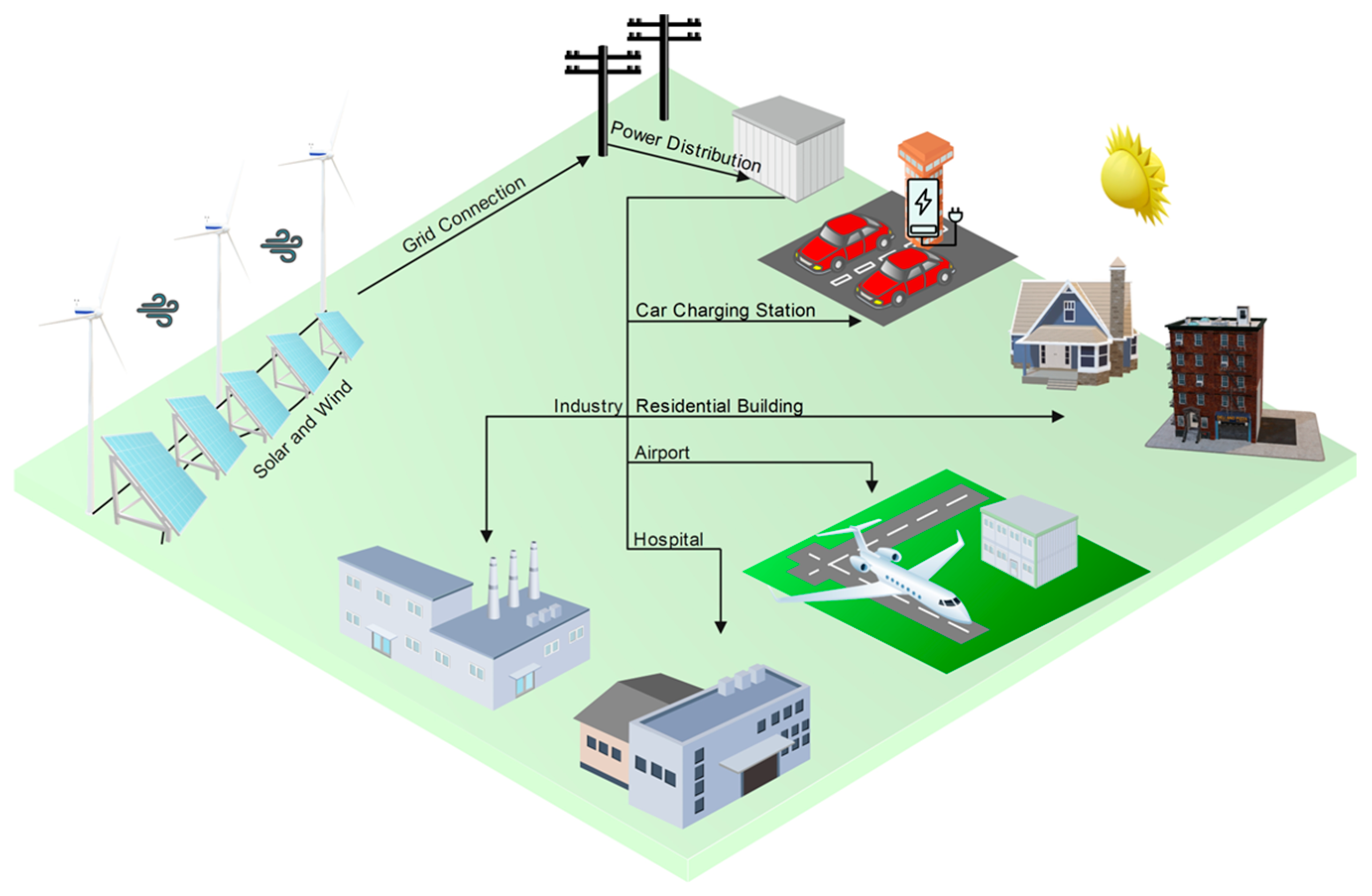
2. Model Site Description and Data Collection

To validate the accuracy of the proposed Fourier neural network method, we consider the case of the city of Midland, TX, positioned at a latitude of 31.9974° N and a longitude of 102.0779° W, as shown in Figure 1. Texas, renowned for its abundant solar and wind potential across all seasons, is a good location for this evaluation. The dataset used for the validation and training phases in this analysis was sourced from the National Renewable Energy Laboratory (NREL) website [28]. The comprehensive dataset from the NREL is the foundational source of information for this study, and its solar and wind data provides a reliable basis for model development and evaluation.

3. Regression-Based Fourier Model and Parameter Estimation

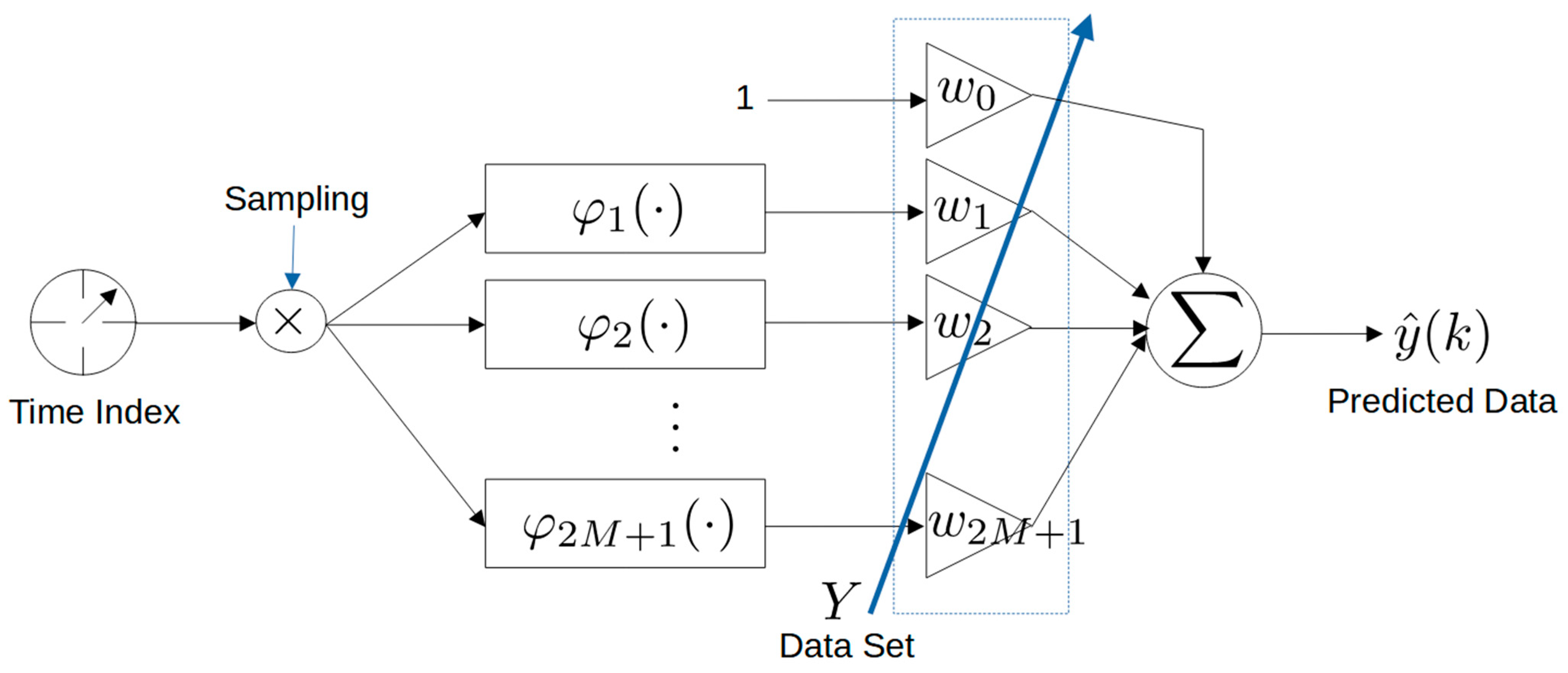
3.1. Regression-Based Fourier Model Formulation

Let y ( t ) be the time-varying signal to be predicted, which is assumed to be quasi-periodic with fundamental frequency ω 0   in radians per time units, for T ( 0 , T d ] the fundamental period, and T d the time duration, with both being given in suitable time units. The fundamental frequency is expressed in Equation (1).
ω 0 = 2 π T
In addition, the signal is sampled at every h time increment, so that the whole signal y ( t ) is described by the vector Y R N that contains the N data points of the given signal, as shown in Equation (2).
Y = [ y 0 ,   y h ,   y 2 h ,     ,   y ( N 1 ) h ]
The signal at the instant t = k h is approximated, or predicted, by the truncated Fourier series expressed in Equation (3):
y ^ k h = 1 2 a 0 + i = 0 M a i cos i ω 0 k h + i = 0 M b i sin i ω 0 k h
where a i and b i are the unknown constant coefficients to be determined, and M is a constant term, such that ω M = M ω 0 remains smaller than the Nyquist frequency expressed in Equation (4):
ω N y q = ω s 2 = π h
This is M < T 2 h N / 2 . A more concise notation is allowed if one defines the vectors as shown in Equation (5):
W = 1 2 a 0 ,   a 1 ,   a 2 ,   , a M ,   b 1 ,   b 2 , ,   b M  
Φ k = [ 1 , cos ω 0 k h , cos 2 ω 0 k h , ,   sin ω 0 k h , sin 2 ω 0 k h ,   ] T
Thus, the result is in the following Equation (7):
y ^ k h = W   Φ k
It can be condensed in a matrix-vector product, as shown in Equation (8).
Y ^ = W Φ
where Φ R ( 2 M + 1 ) × N is the regressor matrix, whose k-th column is Φ k .
The coefficients can be found in Equation (9) by using the damped pseudo-inverse matrix.
Φ # = Φ T ( Φ Φ T + ε I ) 1
If there is a sufficiently small positive ε ; as when the regressor matrix Φ is full-row rank and ε = 0 , it is established that Φ Φ # = I . Then, the coefficients are computed as Equation (10).
W = Y Φ #
The proposed approach then consists of using these same coefficients to estimate the (overall and smooth) behavior of the solar intensity and wind speed, which will make it possible to decide when to activate one or both energy capture systems.
RMSE has been used to measure the accuracy of a predictive model by calculating the square root of the average of squared differences between predicted and actual values, as shown in Equation (11).
R M S E = i n y i y i ^ 2 n
The correlation coefficient measures the strength and direction of a linear relationship between two variables. Two variables, A and B, represent their data points as A i and B i . The correlation coefficient (r) between these two variables is calculated by using the formula Equation (12).
r = ( A i A ¯ ) ( B i B ¯ ) A i A ¯ 2 × ( B i B ¯ ) 2  
The function builds a regressor matrix “phi” on the basis of Fourier series expansion of the input signals. The expansion therefore represents the signal linear variety of Sin and Cos functions with various frequencies. By doing this, the Fourier series expansion gives the function the ability to capture the input signal’s predicted behavior and frequency. The next step is to estimate the parameter “W” by applying an ordinary equation. These parameters describe the weights aligned with each Fourier series sinusoidal component, and these weights help the function models operate between the frequency components and the corresponding time domain values. As long as “W” is estimated, the function builds a regressor matrix for forecasting future values. In addition, using this regressor matrix and learned parameters can help to predict the future signal in the time domain.

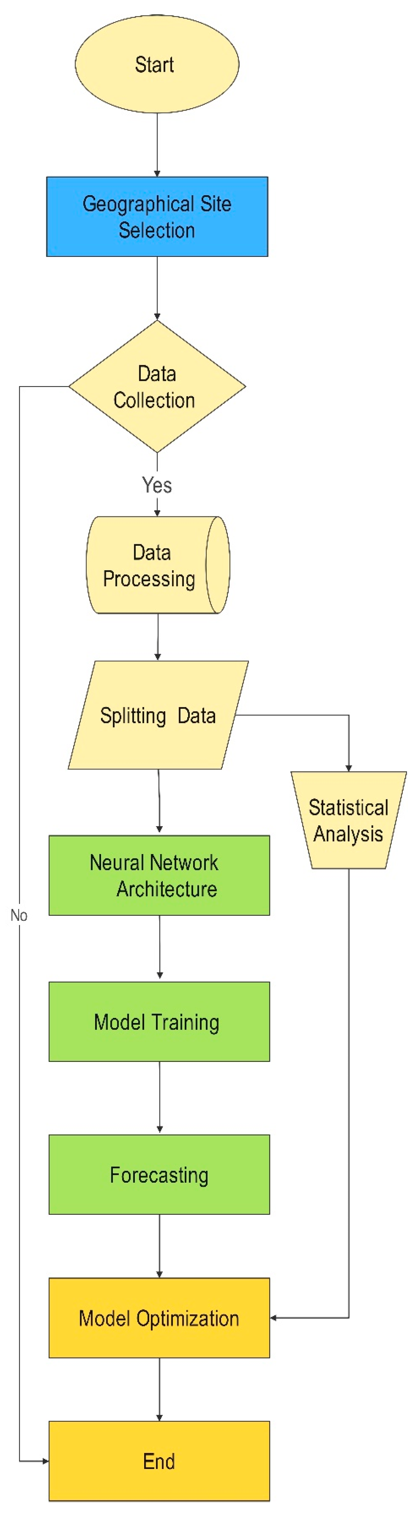
3.2. General Model Description

Electricity plays a significant role in both residential and commercial buildings, with the residual sector accounting for 44% of total electrical consumption [30]. At present, the grid is a mix of various energy sources, such as natural gas, solar, wind, and nuclear energy. In order to achieve a net zero carbon emission goal, there is a need to decarbonize and electrify all residential and commercial buildings. Researchers therefore need to consider the available infrastructure and focus on the number of wind turbines and solar PVs in order to meet the target shown in Figure 2.
The hierarchical methodology employed for predicting the DNI, DHI, and wind speed follows a systematic approach to ensure precise and effective forecasting. The initial step involves meticulously choosing the geographical site for forecasting meteorological data, while taking into account the distinct patterns observed in different locations. Once the site is identified, the subsequent phase involves amassing comprehensive data for wind speed, DNI, and DHI, and doing the groundwork for training, validating, and testing the predictive model. The gathered data then undergoes preprocessing to cleanse and organize it efficiently, addressing missing values, normalizing variables, and preparing the dataset for input into the prediction model. Subsequently, the dataset is partitioned into training, validation, and testing sets, with the training set used for model training, the validation set used to aid the fine-tuning of parameters, and the testing set used to evaluate the model’s unseen data performance. Hierarchical neural network architectures are then crafted for predicting wind speed, DNI, and DHI, which involves the development of distinct networks for each parameter, while ensuring connectivity for efficient information transfer. The model undergoes training using a training dataset, with adjustments iteratively made to weights and biases to minimize prediction errors and enhance the dataset’s ability to capture intricate relationships within the data. After training, the model predicts future values of wind speed, DNI, and DHI by inputting new or unseen data for the selected geographical site. A comprehensive statistical analysis follows forecasting to evaluate the efficiency and accuracy of the model, calculating metrics such as RMSE and correlation coefficients. Continual adjustments are made on the basis of the statistical analysis to optimize the model for enhanced accuracy. This hierarchical approach guarantees a methodical process for constructing, training, and assessing the predictive model. Ultimately the goal is to improve its accuracy and applicability in real-world meteorological forecasting, as depicted in Figure 3.
The structure of the Fourier series-based network is shown in Figure 4. For each time index, when the sampling time is known, the data is predicted as a linear combination of sines and cosines. This is a linear combination of the functions φ i ( · ) , where the coefficients for such linear combination use both the measure data (training set) and the given approximation functions. After the training phase, these coefficients are considered to forecast solar irradiance and wind speed for decision-making purposes.

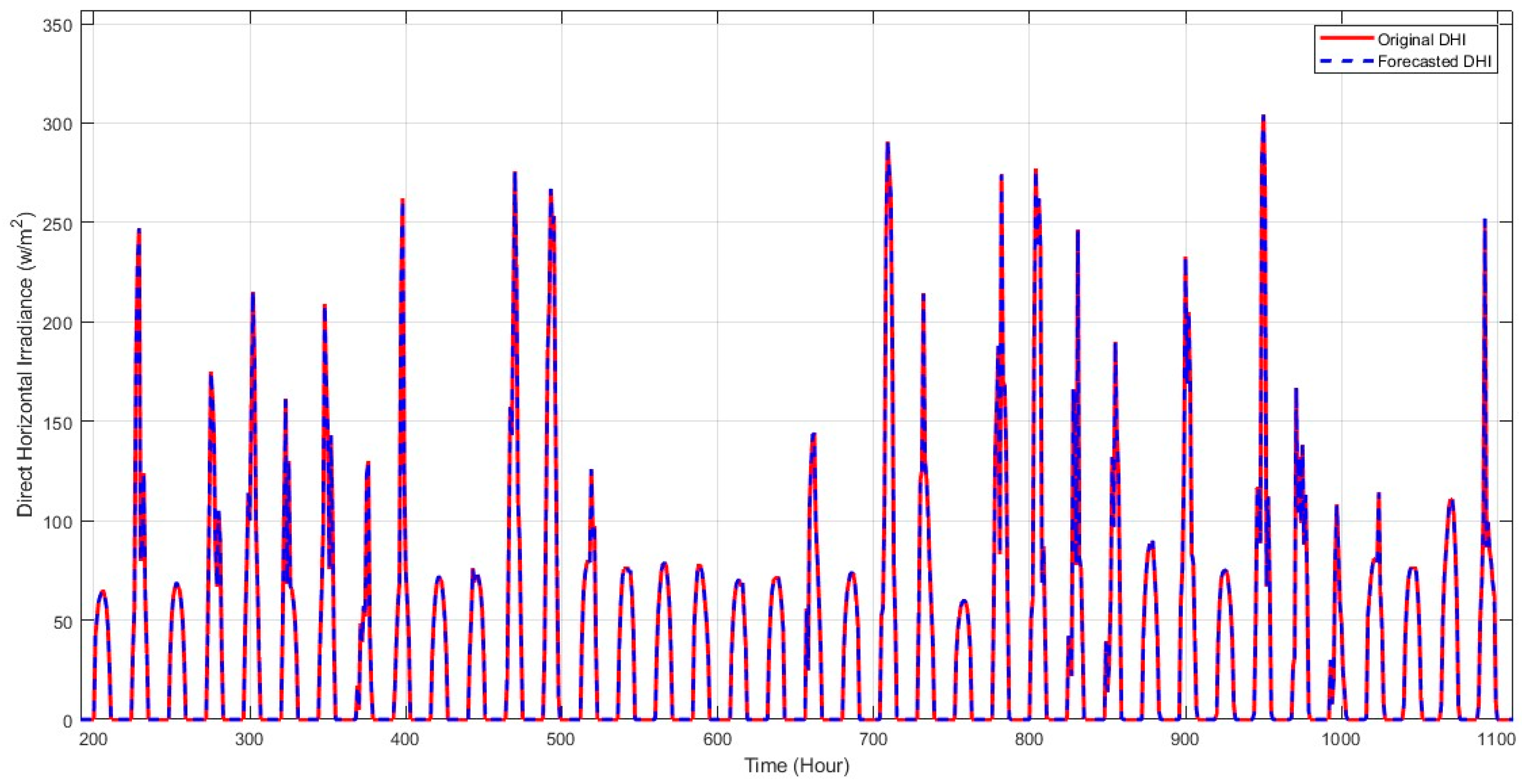
4. Results and Discussions

In designing a renewable energy system, it is necessary to calculate the required number of solar panels or wind turbines. Having an incomplete data set for wind speed can therefore affect the techno-economic analysis, although it should also be acknowledged that the number of turbines is determined on the basis of the wind speed in the needed area. Conversely, solar PV design requires the DNI and DHI, which are two parameters that are key to finding the global horizontal irradiance (GHI). These three parameters show how much solar radiation can reflect on the PV panel.
In this study, the Fourier network regression model shows its proficiency in predicting key meteorological variables (DHI, DNI, and wind speed) across the entire 8760 h duration of the year. The visual representation in Figure 5 and Figure 6 emphasized the model’s accuracy in forecasting DHI and DNI, showing a good alignment between the predicted and observed data points that highlighted its ability to effectively capture solar radiation patterns.
In zooming in on the DHI and DNI, Figure 7 and Figure 8 provided a detailed examination of the model’s performance in replicating the nuances of horizontal solar irradiance. The close correspondence between the predicted and actual DHI and DNI values underscored the model’s ability to capture the subtleties of this specific meteorological parameter.
The analysis was expanded to include wind speed predictions. Figure 9 and Figure 10 offered insights into the model’s effectiveness in anticipating wind patterns. Visual comparison revealed a commendable accuracy in predicting wind speed variations, further reinforcing the model’s reliability in handling diverse meteorological phenomena.
The collective success observed across meteorological parameters in Figure 5, Figure 6, Figure 7, Figure 8, Figure 9 and Figure 10 highlights the adaptability of the Fourier network regression model, and the results position the model as a valuable tool for renewable energy. Forecast provides nuanced insights that can be used to optimize energy systems and support informed decision-making.
Figure 11 displays the magnitude spectrum, representing the amplitude of components at specific frequencies, scaled by multiples of the fundamental frequency. With a fundamental frequency set at one event per year, the results reveal pronounced fluctuations that align with sun activity, exhibiting variations throughout the day and night, and vice versa.
The phase behavior in Figure 12 fluctuates due to factors like noise, fundamental frequency uncertainties, and non-integer multiples frequency components, making phase inference challenging. However, addressing the ensuing complexity is beyond the scope of this paper.
The residual figures for both DHI and DNI show slight differences, which are commonly referred to as “noise,” and this is particularly noticeable within the middle segment of the dataset. Despite these minor variations, it is important to note the overall performance of the Fourier network regression model remains commendable, underscoring its capacity to accurately predict solar radiation across diverse conditions. In the context of these residual figures, “noise” signifies the slight differences between the model’s predictions and the actual observed values. The numerical range of the residuals indicates the discrepancies are of relatively small magnitude. A thorough assessment of the data within a specific range is recommended to further refine the model’s predictive capabilities. Detailed analysis aims to identify conditions or factors contributing to the observed “noise”, facilitating precise adjustments of the model parameters. In summary, the minor “noise” in the residuals poses a manageable challenge that can be strategically addressed by focused model refinement. The broader context suggests the model accurately predicts DHI and DNI across most of the dataset. Strategic adjustments based on the detailed analysis of the middle portion of the data can contribute to an even more refined and precise forecasting model for solar irradiance—Figure 13, Figure 14 and Figure 15 shows residuals for DHI, DNI, and wind speed.
The histograms of the residuals for the DHI, DNI, and wind speed reveal distinctive patterns in the distribution of the model’s prediction errors. In the case of DHI (Figure 16), the histogram skews to the left, indicating a concentration of residuals around lower values, with the highest peak centered around or near the zero axis. This suggests the model tends to slightly overestimate the DHI. The predominance of values closer to zero, meanwhile, emphasizes the model’s generally accurate predictions of minor discrepancies.
In contrast, the DNI histogram (Figure 17) displays a broader distribution with a symmetrical shape, and is centered on the zero axis. The distribution shows a balanced spread of residuals, indicating the model’s predictions of the DNI include a mixture of overestimations and underestimations.
The symmetrical pattern implies a well-distributed range of errors. The wind speed histogram (Figure 18) has a unique form with a single line at zero; in emphasizing t, the model tends to have minimal discrepancies, especially around the zero axis. This suggests a high level of accuracy in predicting wind speed, with deviations from the actual observations being notably minor. Despite the small values on the x-axis, visualizations effectively communicate the nuanced distribution of residuals for each parameter. The concentration of values around zero underscores the model’s precision, and deviations are minor when considered in the wider context of the scale of the data. Hereafter, the insights provide a foundation for further refinements that will help to ensure the model aligns closely with observed values across the spectrum.
RMSE is a common metric used to measure errors, whose application to energy data is highly recommended [31]. The RMSE values for the wind speed, DNI, and DHI quantitatively assess the model’s performance in predicting these meteorological parameters. The RMSE is 0.0007555, indicating a relatively low error in the model’s predictions, as shown in Figure 19. Overall, the low RMSE values across wind speed, DNI, and DHI indicate that the Fourier network regression model’s prediction of these meteorological parameters is highly effective and reliable. The model’s performance supports its utility in renewable energy forecasting and meteorological analysis applications, as its small RMSE value affirms.
The correlation values of one model indicate a perfect positive linear relationship between the model predictions and the actual observed values for each respective meteorological parameter. Ideal correlation suggests the model accurately captures the variations and trends in wind speed, DNI, and DHI, and also that the predicted values are directly proportional to the observed values. In addition, the correlation values of one model show the Fourier network regression model’s prediction of the three parameters is both accurate and robust.

5. Conclusions

A Fourier network regression model was implemented to examine solar intensity and wind speed data, and it demonstrated impressive accuracy in predicting and recovering data. Validation of the model was conducted using NREL data and statistical techniques, affirming its capability to optimize energy system configurations. The proposed hierarchical approach encompassed site selection, data collection, and neural network development, producing outcomes that underscored the model’s dependability, including minimal RMSE values. Residual analysis identified minor discrepancies, offering insights for potential future enhancements. In summary, the Fourier network regression model emerges as an asset for forecasting renewable energy data that will facilitate sustainable energy systems design.

Author Contributions

Conceptualization, A.F.A.-A. and A.J.M.V.; methodology, A.F.A.-A.; software, A.F.A.-A. and A.J.M.V.; validation, A.F.A.-A.; formal analysis, A.F.A.-A.; investigation, A.F.A.-A. and A.J.M.V.; resources, F.Y.A.-A.; writing—original draft, A.F.A.-A. and F.Y.A.-A.; writing—review & editing, A.F.A.-A., A.J.M.V., F.Y.A.-A., M.E.-H. and W.Z.; visualization, A.F.A.-A.; supervision, F.Y.A.-A., M.E.-H. and W.Z. All authors have read and agreed to the published version of the manuscript.

Funding

This research received no external funding.

Institutional Review Board Statement

Not applicable.

Informed Consent Statement

Not applicable.

Data Availability Statement

Data are contained within the article.

Conflicts of Interest

The authors declare no conflicts of interest.

Abbreviation

A i , B i Individual data points for variables A and B, respectively.
A ^   a n d   B ^ The means of variables A and B.
y(t)The signal that changes over time and needs to be predicted.
T d The signal’s total time duration l.
hThe time increment between each signal sample.
kAn index representing a specific time instant.
a 0 , a i , b i Unknown constant coefficients in a mathematical series used for prediction.
ω N y q The Nyquist frequency, half of the sampling angular frequency ω s .
NThe number of data points in the signal.
Φ k A vector used in the prediction process.
y ^ A vector representing the predicted signal.
ϵA small positive constant.
TThe fundamental period of the signal.
ω 0 The fundamental angular frequency.
YA vector containing all the signal’s sampled data points.
y ^ k h The predicted or approximated signal at a specific time instant.
MA constant term in the mathematical series.
ω s The angular frequency at which the signal is sampled.
WA vector containing coefficients used for prediction.
Φ A matrix of vectors used in the prediction process.
Φ # A mathematical operation involving the pseudo-inverse matrix.
IThe identity matrix.
nThe number of observations in the dataset.
y i The actual values.
y i ^ The predicted values.

References

  1. Strazzabosco, A.; Kenway, S.J.; Lant, P.A. Solar PV adoption in wastewater treatment plants: A review of practice in California. J. Environ. Manag. 2019, 248, 109337. [Google Scholar] [CrossRef] [PubMed]
  2. Bey, M.; Hamidat, A.; Nacer, T. Eco-energetic feasibility study of using grid-connected photovoltaic system in wastewater treatment plant. Energy 2021, 216, 119217. [Google Scholar] [CrossRef]
  3. Zhang, Y.; Pinoy, L.; Meesschaert, B.; Van der Bruggen, B. A natural driven membrane process for brackish and wastewater treatment: Photovoltaic powered ED and FO hybrid system. Environ. Sci. Technol. 2013, 47, 10548–10555. [Google Scholar] [CrossRef] [PubMed]
  4. Al-Aboosi, F.Y.; Al-Aboosi, A.F. Preliminary Evaluation of a Rooftop Grid-Connected Photovoltaic System Installation under the Climatic Conditions of Texas (USA). Energies 2021, 14, 586. [Google Scholar] [CrossRef]
  5. Al-Aboosi, F.Y. Models and hierarchical methodologies for evaluating solar energy availability under different sky conditions toward enhancing concentrating solar collectors use: Texas as a case study. Int. J. Energy Environ. Eng. 2020, 11, 177–205. [Google Scholar] [CrossRef]
  6. Yadav, A.K.; Chandel, S. Solar radiation prediction using Artificial Neural Network techniques: A review. Renew. Sustain. Energy Rev. 2014, 33, 772–781. [Google Scholar] [CrossRef]
  7. Sharma, N.; Sharma, P.; Irwin, D.; Shenoy, P. Predicting solar generation from weather forecasts using machine learning. In Proceedings of the 2011 IEEE International Conference on Smart Grid Communications (SmartGridComm), Brussels, Belgium, 17–20 October 2011. [Google Scholar]
  8. Jebli, I.; Belouadha, F.-Z.; Kabbaj, M.I.; Tilioua, A. Prediction of solar energy guided by pearson correlation using machine learning. Energy 2021, 224, 120109. [Google Scholar] [CrossRef]
  9. Torabi, M.; Mosavi, A.; Ozturk, P.; Varkonyi-Koczy, A.; Istvan, V. A hybrid machine learning approach for daily prediction of solar radiation. In Recent Advances in Technology Research and Education: Proceedings of the 17th International Conference on Global Research and Education Inter-Academia–2018, Kaunas, Lithuania, 24–27 September 2018; Springer: Berlin/Heidelberg, Germany, 2019. [Google Scholar]
  10. Hassan, M.Z.; Ali, M.E.K.; Ali, A.S.; Kumar, J. Forecasting day-ahead solar radiation using machine learning approach. In Proceedings of the 2017 4th Asia-Pacific World Congress on Computer Science and Engineering (APWC on CSE), Mana Island, Fiji, 11–13 December 2017. [Google Scholar]
  11. González-Plaza, E.; García, D.; Prieto, J.-I. Monthly Global Solar Radiation Model Based on Artificial Neural Network, Temperature Data and Geographical and Topographical Parameters: A Case Study in Spain. Sustainability 2024, 16, 1293. [Google Scholar] [CrossRef]
  12. Xu, L.; Li, Y.; Wang, X.; Liu, L.; Ma, M.; Yang, J. A Machine Learning Approach to Estimating Solar Radiation Shading Rates in Mountainous Areas. Sustainability 2024, 16, 931. [Google Scholar] [CrossRef]
  13. Wang, J.; Zhang, W.; Wang, J.; Han, T.; Kong, L. A novel hybrid approach for wind speed prediction. Inf. Sci. 2014, 273, 304–318. [Google Scholar] [CrossRef]
  14. Chang, W.-Y. A literature review of wind forecasting methods. J. Power Energy Eng. 2014, 2, 161. [Google Scholar] [CrossRef]
  15. DuVivier, K.; Mooney, B.T. Moat Mentality: Onshore and Offshore Approaches to Wind Waking. Notre Dame J. Emerg. Tech. 2020, 1, 1. [Google Scholar]
  16. Hemami, A. Wind Turbine Technology; Cengage Learning: Clifton Park, NY, USA, 2012. [Google Scholar]
  17. Delgado, I.; Fahim, M. Wind turbine data analysis and LSTM-based prediction in SCADA system. Energies 2020, 14, 125. [Google Scholar] [CrossRef]
  18. He, Y.; Kusiak, A. Performance assessment of wind turbines: Data-derived quantitative metrics. IEEE Trans. Sustain. Energy 2017, 9, 65–73. [Google Scholar] [CrossRef]
  19. Becker, R.; Thrän, D. Completion of wind turbine data sets for wind integration studies applying random forests and k-nearest neighbors. Appl. Energy 2017, 208, 252–262. [Google Scholar] [CrossRef]
  20. Zhao, X.; Wang, S.; Li, T. Review of evaluation criteria and main methods of wind power forecasting. Energy Procedia 2011, 12, 761–769. [Google Scholar] [CrossRef]
  21. Wu, Y.-K.; Hong, J.-S. A literature review of wind forecasting technology in the world. In Proceedings of the 2007 IEEE Lausanne Power Tech, Lausanne, Switzerland, 1–5 July 2007; pp. 504–509. [Google Scholar]
  22. Lei, M.; Shiyan, L.; Chuanwen, J.; Hongling, L.; Yan, Z. A review on the forecasting of wind speed and generated power. Renew. Sustain. Energy Rev. 2009, 13, 915–920. [Google Scholar] [CrossRef]
  23. Firat, U.; Engin, S.N.; Saraclar, M.; Ertuzun, A.B. Wind speed forecasting based on second order blind identification and autoregressive model. In Proceedings of the 2010 Ninth International Conference on Machine Learning and Applications, Washington, DC, USA, 12–14 December 2010. [Google Scholar]
  24. Guo, Z.-h.; Wu, J.; Lu, H.-y.; Wang, J.-z. A case study on a hybrid wind speed forecasting method using BP neural network. Knowl. Based Syst. 2011, 24, 1048–1056. [Google Scholar] [CrossRef]
  25. Faria, D.L.; Castro, R.; Philippart, C.; Gusmao, A. Wavelets pre-filtering in wind speed prediction. In Proceedings of the 2009 International Conference on Power Engineering, Energy and Electrical Drives, Lisbon, Portugal, 18–20 March 2009. [Google Scholar]
  26. Che, G.; Zhou, D.; Wang, R.; Zhou, L.; Zhang, H.; Yu, S. Wind Energy Assessment in Forested Regions Based on the Combination of WRF and LSTM-Attention Models. Sustainability 2024, 16, 898. [Google Scholar] [CrossRef]
  27. Rueda-Bayona, J.G.; Cabello Eras, J.J.; Sagastume, A. Modeling Wind Speed with a Long-Term Horizon and High-Time Interval with a Hybrid Fourier-Neural Network Mode. Available online: https://www.iieta.org/journals/mmep/paper/10.18280/mmep.080313 (accessed on 2 January 2024).
  28. Laboratory, S.E. National Solar Radiation Data Base Sites for Texas. 2024. Available online: http://www.me.utexa (accessed on 2 January 2024).
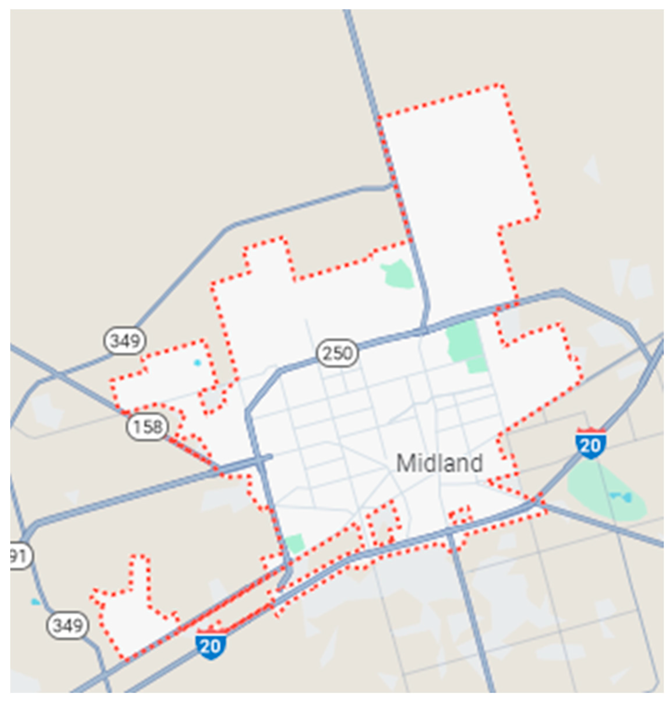
  29. Midland Map. 2023. Available online: https://www.google.com/maps (accessed on 3 December 2023).
  30. EIA—U.S. Energy Information Administration. Use of Energy in Homes.Energy Explained. Available online: https://www.eia.gov/energyexplained/use-of-energy/homes.php (accessed on 12 February 2024).
  31. Lee, M.H.L.; Ser, Y.C.; Selvachandran, G.; Thong, P.H.; Cuong, L.; Son, L.H.; Tuan, N.T.; Gerogiannis, V.C. A Comparative Study of Forecasting Electricity Consumption Using Machine Learning Models. Mathematics 2022, 10, 1329. [Google Scholar] [CrossRef]
Figure 1. Case study Location, Midland, TX, USA [29].
Bdcc 08 00023 g001
Figure 2. Integrating Solar and Wind Power Into the Existing Electric Grid.
Bdcc 08 00023 g002
Figure 3. A Hierarchical Methodology for Predicting DNI, DHI, and Wind Speed.
Bdcc 08 00023 g003
Figure 4. Fourier Series-based Network.
Bdcc 08 00023 g004
Figure 5. Original DHI versus Forecasted DHI.
Bdcc 08 00023 g005
Figure 6. Original DNI versus Forecasted DNI.
Bdcc 08 00023 g006
Figure 7. Zoomed-in Original DHI versus Forecasting DHI.
Bdcc 08 00023 g007
Figure 8. Zoomed-in Original DNI versus Forecasted DNI.
Bdcc 08 00023 g008
Figure 9. Original Wind Speed versus Forecasted Wind Speed.
Bdcc 08 00023 g009
Figure 10. Zoomed-In Original Wind Speed versus Forecasted Wind Speed.
Bdcc 08 00023 g010
Figure 11. Magnitude Spectrum.
Bdcc 08 00023 g011
Figure 12. Phase Spectrum.
Bdcc 08 00023 g012
Figure 13. DHI Residuals.
Bdcc 08 00023 g013
Figure 14. DNI Residuals.
Bdcc 08 00023 g014
Figure 15. Wind Speed Residuals.
Bdcc 08 00023 g015
Figure 16. Histogram of DHI residuals.
Bdcc 08 00023 g016
Figure 17. Histogram of DNI Residuals.
Bdcc 08 00023 g017
Figure 18. Histogram of wind speed residuals.
Bdcc 08 00023 g018
Figure 19. RMSE with Different Adjustment.
Bdcc 08 00023 g019
Disclaimer/Publisher’s Note: The statements, opinions and data contained in all publications are solely those of the individual author(s) and contributor(s) and not of MDPI and/or the editor(s). MDPI and/or the editor(s) disclaim responsibility for any injury to people or property resulting from any ideas, methods, instructions or products referred to in the content.

