Article

Forecasting Human Core and Skin Temperatures: A Long-Term Series Approach

1
School of Emergency Management & Safety Engineering, China University of Mining and Technology, Beijing 100083, China
2
Inner Mongolia Research Institute, China University of Mining and Technology (Beijing), Ordos 017004, China
3
Empa, Swiss Federal Laboratories for Materials Science and Technology, Laboratory for Biomimetic Membranes and Textiles, CH-9014 St. Gallen, Switzerland
*
Author to whom correspondence should be addressed.
Big Data Cogn. Comput. 2024, 8(12), 197; https://doi.org/10.3390/bdcc8120197
Submission received: 20 September 2024 / Revised: 11 December 2024 / Accepted: 17 December 2024 / Published: 19 December 2024

Abstract

:
Human core and skin temperature (Tcr and Tsk) are crucial indicators of human health and are commonly utilized in diagnosing various types of diseases. This study presents a deep learning model that combines a long-term series forecasting method with transfer learning techniques, capable of making precise, personalized predictions of Tcr and Tsk in high-temperature environments with only a small corpus of actual training data. To practically validate the model, field experiments were conducted in complex environments, and a thorough analysis of the effects of three diverse training strategies on the overall performance of the model was performed. The comparative analysis revealed that the optimized training method significantly improved prediction accuracy for forecasts extending up to 10 min into the future. Specifically, the approach of pretraining the model on in-distribution samples followed by fine-tuning markedly outperformed other methods in terms of prediction accuracy, with a prediction error for Tcr within ±0.14 °C and Tsk, mean within ±0.46 °C. This study provides a viable approach for the precise, real-time prediction of Tcr and Tsk, offering substantial support for advancing early warning research of human thermal health.

1. Introduction

Human core and skin temperature (Tcr and Tsk) are crucial indicators of human health and are commonly utilized in assessing thermal health risks. There are two types of body temperature: core temperature (Tcr) and skin temperature (Tsk). Tcr is primarily used for diagnostic purposes due to the availability of clear standards [1]. However, measuring Tcr is complex and inevitably burdensome. In contrast, Tsk, which can vary based on individual differences, activity, and environmental temperatures, lacks uniform standards. Nonetheless, abnormal changes in Tsk can still reflect the thermal risk faced by an individual. If assessed properly, Tsk can provide researchers with valuable information regarding organ function, blood flow, and thermoregulation [2]. Moreover, Tsk can be measured using simple methods, including wearable devices such as wristbands, making it more suitable for daily early warning of thermal health to humans.
The human body has a complex regulatory mechanism to maintain body temperature within a relatively stable range, including heat production, heat dissipation, and behavioral adjustment, etc. [3,4,5,6,7,8,9,10,11,12]. Traditionally, by simulating the physical laws of this regulation, one can predict the Tcr and Tsk of the human body under specific environmental conditions. These models can predict the Tcr and Tsk of the human body under specific conditions, and their effectiveness is based on accurately reproducing the body’s response to environmental changes. However, in practice, the thermal exchange processes of the human body are often more complex. In addition to basic universal environmental factors and human conditions, many other variables such as medication use, illness, diet, and sleep can also influence human thermal exchange. Therefore, these models face challenges when considering individual differences [13]. Moreover, to accurately simulate the thermal exchange of the human body, these models often have complex structures and require more input parameters, which may pose difficulties in practical applications [14]. Thus, in many complex application scenarios, accurately predicting personalized Tcr and Tsk of the human body remains an out of reach goal [15].
Another study on predicting Tcr and Tsk employed a data-driven approach. These approaches significantly reduce the need for subjective experience, consider a wider range of influencing factors, and offer more objective model performance, making them more applicable to a broader and more complex range of scenarios. Current studies on data-driven-based human physiological indicator prediction primarily focus on predicting Tcr, Tsk, heart rate and thermal health [16,17,18,19,20,21]. However, privacy and security concerns may make it difficult to obtain large-scale public datasets of Tcr and Tsk, especially under extreme conditions, limiting researchers’ ability to independently train efficient predictive warning models. Considering both aspects, the method of physical modeling can provide the physical laws in human thermal response, which can then be personalized and adjusted for complex environments in data-driven approaches. Therefore, these two methods should be considered complementary.
In the face of current challenges, the combination of Long-Term Series Forecasting (LTSF) models and transfer learning (TL) technique presents a powerful solution. LSTF requires models to have high predictive capabilities, effectively capturing the precise long-range dependencies between outputs and inputs. It allows for long-term ahead forecasting while maintaining prediction accuracy. Currently, such models have been applied in traffic prediction [22], spectrum forecasting [23], power forecasting [24,25], and mechanical lifetime prediction [26], achieving good prediction results. If this forecasting method could be applied to human thermal strain prediction, it could predict potential thermal strain events in advance, providing users with ample time to react and respond, thereby significantly reducing the likelihood of thermal strain and ensuring users’ health. TL is a machine learning technique that allows a model trained on one task to be reused for a new, but related, task. Based on this technology, it is possible to leverage the knowledge of a pre-trained model, avoiding the need to build and train a model from scratch, thus saving substantial computational resources and time. Transfer learning has already been successfully applied in various machine learning applications, including text sentiment classification [27], image classification [28,29,30,31], human activity classification [32,33], software defect classification [34,35,36,37], and multilingual text classification [38,39,40]. Particularly with the widespread use of wearable health monitoring devices, transfer learning technology from “source domain” to “target domain”—i.e., training a model on one dataset and applying it to another dataset—offers a robust solution to the problem of insufficient data in the field of human temperature prediction. The core idea of this method is that the knowledge learned from the source domain can help the model perform better on the target domain task, especially when annotated data are scarce or completely unavailable in the target domain. This approach is particularly suitable for situations where the target task in human temperature prediction has limited data available, but a large amount of data are needed to train an effective model.
Here, we propose a prediction model of Tcr and Tsk that integrates LTSF methods with TL technology. This model initially undergoes pretraining using data generated by traditional human thermo-physiological models. Subsequently, a 72 h field experiment in high-temperature conditions is conducted, during which real-world observational data are collected to fine-tune the model. This fine-tuning enhances the accuracy of long-term predictions, enabling personalized real-time predictions of Tcr and Tsk. The model operates independently of environmental parameters, human parameters, and clothing parameters, relying solely on long-term monitoring data of historical skin temperature and core temperature to forecast future Tcr and Tsk. This capability allows for timely warnings in high-temperature working environments, providing ample time for hazard avoidance and response. In the final model evaluation phase, the model is evaluated using data collected from field experiments conducted in complex high-temperature environments. The evaluation includes testing the impact of three primary different training methods on the model’s performance.

2. Materials and Methods

In this study, long-term human temperature forecasting is conducted through the integration of the LTSF model with TL technology. Figure 1 shows our methodological framework.

2.1. Methods

2.1.1. Thermo-Physiological Model

JOS-3 has been widely used as an open-source thermo-physiological model. In this study, the JOS-3 model is used as the generation model for simulated data. The JOS-3 thermo-physiological model [41] is employed in this study as the pretraining data generation model. The model is based on the Stolwijk model [42], composed of 83 nodes and calculates human physiological responses and temperatures using the finite difference method. A key feature of the model is its consideration of individual characteristics in transient and nonuniform thermal environments, offering high simulation accuracy and flexibility in complex settings.
The development of the JOS-3 model was aimed at predicting human physiological responses while accounting for individual characteristics in transient and nonuniform thermal environments. The body is divided into the following 17 parts: head, neck, chest, back, pelvis, L-shoulder, L-arm, L-hand, R-shoulder, R-arm, R-hand, L-thigh, L-leg, L-foot, R-thigh, R-leg, and R-foot [41]. To date, JOS-3 has been validated in low-metabolic indoor environments [41] and is capable of predicting temperatures across different body segments, mean skin temperature (Tsk,mean), and Tcr. Additionally, JOS-3 has been validated for accurately simulating increases in Tcr across six sports: athletics, soccer, rowing, rugby, tennis, and triathlon [43]. The model has been widely used in recent years [44,45,46,47,48]. The model’s accuracy is further demonstrated by the mean absolute error (MAE) and root mean square error (RMSE) values. For Tcr, the MAE and RMSE ranged from 0.13 to 0.37 °C and 0.12 to 0.38 °C, respectively [41]. For Tsk,mean, the MAE and RMSE were found to range from 0.47 to 0.68 °C and 0.58 to 0.83 °C, respectively. These errors indicate that the model provides reliable predictions for both Tcr and Tsk in various thermal environments.

2.1.2. Informer

The Informer model was introduced in 2021 by Zhou et al. [49] and is based on the Transformer architecture. This model is a Deep Learning (DL) model designed specifically for long-term time series forecasting, with significant improvements in efficiency and accuracy when handling long-sequence data. Compared to the Transformer, the Informer utilizes an efficient self-attention mechanism, improving the attention mechanism and addressing the issues of quadratic time complexity and quadratic memory usage. The encoder–decoder configuration of the Informer enables the capture of information from long-sequence time series.
Specifically, the Transformer adopts the classic encoder–decoder structure, where the encoder is responsible for encoding the input sequence into a contextual representation, and the decoder generates the output based on the encoded context. Specifically, in the standard Transformer, both the encoder and decoder use the same self-attention mechanism, which calculates attention scores for all positions in the sequence. In long-sequence tasks, the computational cost of this attention mechanism increases dramatically with the length of the sequence, leading to inefficiency, especially when dealing with long sequences. The attention computation in both the encoder and decoder becomes a bottleneck in such cases.
In contrast, the Informer optimizes the encoder–decoder configuration. To further reduce redundant computations, the Informer introduces a generative decoder in the decoder section while adopting a more efficient sparse attention mechanism in the encoder. This sparse attention mechanism focuses the computation on the most critical parts of the sequence. These design choices make the model more computationally efficient when handling long time series while still maintaining strong performance in long-term forecasting tasks. The Informer can focus more on important time steps, avoiding unnecessary full-sequence computations, and better capturing critical long-term dependencies. Compared to the traditional Transformer, the Informer is more suitable for long-sequence forecasting tasks because it reduces redundant computations and focuses more on capturing important temporal dependencies.
Overall, the Informer model addresses the efficiency issues of the standard self-attention mechanism in the traditional Transformer model, where the computational complexity on long sequences is quadratic, posing a significant bottleneck for long-sequence time series forecasting.
ProbSparse Self-Attention: In the Informer model, the ProbSparse Self-Attention mechanism is an innovative approach that significantly reduces computational complexity by focusing only on the top ‘ u ’ dominant queries, as determined by a sparsity measurement. Instead of attending to all elements in the sequence, this mechanism selectively computes attention for only the most relevant positions, reducing the number of attention calculations required. The key idea behind ProbSparse Self-Attention is that not all positions in the sequence need to be attended to equally. By using a probabilistic approach, the model identifies and attends to the most important or influential queries, significantly lowering the computational cost, especially for long sequences. This sparse attention mechanism allows the Informer model to efficiently capture long-range dependencies in time-series data while maintaining high performance, making it particularly effective for tasks like predicting human Tcr and Tsk trends and other long-term series problems.
The self-attention calculation is given by the following formula (Formula (1)):
A t t e n t i o n ( Q , K , V ) = S o f t m a x ( Q ¯ K T d ) v
where Attention is the self-attention function, which calculates the attention weights for the input sequence. Q is a sparse matrix containing only the top ‘ u ’ queries determined by the sparsity measure M q ,   K . K is the key matrix used in conjunction with the query matrix for the matching process within the self-attention mechanism. V is the value matrix, which, once the match between queries and keys is established, is used to create a weighted output reflecting the sequence’s important features. d is the dimensionality of the features. In the scaled dot product self-attention mechanism, the dot product of queries and keys is scaled by d to prevent gradients from vanishing or exploding during training. The complexity of this mechanism is O L   l o g   L , which is a significant reduction compared to the quadratic complexity of traditional self-attention.
Regarding the selection of the sparsity threshold and the top ‘ u ’ queries, the Informer does not rely entirely on manually setting these parameters. Instead, it leverages a probabilistic mechanism that dynamically selects sparse connections and the most important query-key pairs. This approach automates the adjustment of these parameters, eliminating the need for fixed, manually set thresholds. Consequently, the model can adapt flexibly to different data characteristics during training, adjusting its sparsity and query selection based on the data at hand. This dynamic adjustment ensures that the model remains robust and maintains high predictive accuracy, even in the presence of extreme values or significant environmental changes, without requiring explicit manual intervention in setting the sparsity threshold. Through this mechanism, the Informer is able to achieve better performance in long-term sequence forecasting tasks while handling complex and varying data effectively.
Sparsity measurement: In the Informer model, the sparsity measurement plays a critical role in enhancing the efficiency of the ProbSparse Self-Attention mechanism by identifying the most important queries to focus on. Instead of attending to all queries equally, this measurement helps determine which queries are the most dominant and should be prioritized during attention computation. By dynamically evaluating the importance of queries, the sparsity measurement ensures that the model focuses on the most relevant parts of the sequence, significantly reducing computational complexity. This selective attention process allows the Informer model to focus on critical points in the sequence, improving its ability to capture long-range dependencies while reducing the computational burden. For tasks like predicting human Tcr and Tsk trends, the sparsity measurement ensures that the model focuses on time steps that have the most impact on future predictions, such as sudden temperature spikes or significant trends, while ignoring less relevant data points.
The sparsity measurement M q i ,   K is defined as shown in Formula (2):
M ( q i , K ) = l n ( j = 1 L K exp ( q i k j d ) ) 1 L K j = 1 L K q i k j d
where q i represents the i th query vector and L K is the number of vectors in the key matrix K . This measure helps identify queries with diverse attention probabilities. Queries with higher sparsity are considered more important in the model and thus are given more focus. This measurement method enables the Informer model to effectively reduce the computational complexity in processing long sequences while maintaining predictive performance.
In the Informer, an encoder is used to efficiently process long sequence inputs.
Self-attention distilling: The encoder applies a distilling operation to focus on dominant features in the self-attention feature map by reducing the time dimension of the input sequence progressively through a combination of Conv1D and max pooling operations, as shown in Formula (3):
X t j + 1 = Max   Pool ( ELU ( Conv 1 d ( [ X t j ] A B ) ) )
where j represents the index of the network layer and X t j + 1 represents the output sequence after the self-attention distilling operation of the j th layer, which is used as an input to the j + 1 layer. [ X t j ] A B denotes the output of X t j after applying the attention block, which typically includes a multi-head ProbSparse Self-Attention mechanism and necessary operations to process the input sequence X t j . Max pooling refers to the max pooling operation, which is used to reduce the spatial dimensions of the data while retaining the most important features. ELU stands for the exponential linear unit activation function. Conv1d is a one-dimensional convolution operation used to extract features along the temporal dimension. This operation reduces memory usage and focuses on the most important features in the sequence.
The decoder of the Informer model adopts a generative approach to efficiently produce long sequence outputs.
Generative inference: Unlike traditional dynamic decoding, the Informer model uses a generative inference approach to generate future predictions in a more efficient manner. Instead of generating the output step-by-step (as in traditional dynamic decoding), the Informer selects a slice of the input sequence as a start token and generates the output in a single forward pass. This approach significantly accelerates the prediction process compared to the step-by-step generation used in conventional models, making it much faster and computationally efficient. This is particularly beneficial for time-series forecasting tasks, where generating long-term predictions from historical data is essential. In this framework, generative inference enables the model to predict the entire future sequence at once, capturing the uncertainty and complexity of the time-series data. This is crucial for tasks like predicting human Tcr and Tsk trends, where factors like daily cycles, physiological changes, and environmental influences need to be accounted for. By leveraging a single forward pass, the Informer model can generate predictions over long sequences without the computational overhead of sequential decoding. Additionally, this method allows the model to generate a range of plausible future values, rather than relying on deterministic outputs, thereby modeling the inherent uncertainty in the data more effectively. The generative inference approach helps the model handle long-range dependencies and fluctuations in time-series data, offering more robust predictions.
The process is mathematically expressed as shown in Formula (4):
X t d e = Concat ( X t t o k e n , X t 0 )
where X t d e is the input to the decoder. This matrix is formed by concatenating parts X t t o k e n and X t 0 , which represent the data to be processed by the decoder. X t t o k e n is the start token, a known sequence preceding the target sequence, used as the initial input for the decoder. X t 0 is a placeholder for the target sequence, serving to reserve space for the sequence that the model needs to predict. This method allows the decoder to generate predictions for the entire sequence in a single forward propagation step, enhancing the efficiency of long-sequence forecasting.
Loss function: The model uses the mean squared error (MSE) as the loss function for training, optimizing the predictions with respect to the target sequences.
During the research process, some necessary adjustments were made to the hyperparameters of the Informer. The adjusted hyperparameters are shown in Appendix A (Table A1).

2.1.3. Transfer Learning

TL is an ML technique that allows a model trained on one task to be repurposed for a new but related task. Leveraging the knowledge from pretrained models can circumvent the need to build and train models from scratch. The core idea of TL is that under certain circumstances, knowledge learned from the source task can still be beneficial in the target task, even if the source and target tasks are not entirely identical. This approach is particularly suited to situations where the target task has limited data available but requires substantial data to train an effective model.
The main steps and principles of TL include the following:
Pretraining phase: In this stage, the model is trained on the source task. The source task is typically a data-rich task, allowing the model to learn rich feature representations.
Transfer and adaptation: In this phase, the pretrained model is applied to the target task. This usually involves making modifications to the model to better adapt it to the target task.
Fine-tuning: After transfer, the model is often further trained on target task data to fine-tune the model parameters, making it better suited to the target task. This step can be adjusted based on the amount and complexity of the target task data.
The advantages of TL lie in its ability to save significant amounts of training time and resources, especially in domains where data are scarce. Moreover, TL enables models to leverage knowledge obtained from related tasks, thereby achieving better performance on new tasks. Furthermore, TL also helps enhance the model’s generalizability across different tasks.
In this research, TL was utilized to enhance the model’s performance. Initially, the model was pretrained using synthetic data generated from traditional human thermo-physiological models. This pretraining phase allowed the model to learn general patterns and feature representations related to human temperature regulation. Subsequently, the pretrained model was fine-tuned using real-world observational data collected during a 72 h field experiment conducted under high-temperature conditions. This fine-tuning significantly improved the model’s ability to make accurate long-term predictions and enabled personalized, real-time forecasting of human Tcr and Tsk.

2.1.4. Evaluation of the Model Performance

The model performance is evaluated using the RMSE, MAE, MAPE and R-squared (R2) metrics.
The RMSE amplifies prediction errors through squared terms, placing greater emphasis on larger errors, and is highly sensitive to outliers. The RMSE calculation formula is as shown in Formula (5):
R M S E = 1 n i = 1 n ( y i y ^ i ) 2
where y i represents the actual values, y ^ i represents the predicted values, and n is the number of samples.
The MAE assigns equal weight to all errors without emphasizing large errors, providing a robust estimate of error, as shown in Formula (6).
M A E = 1 n i = 1 n | y i y ^ i |
The MAPE assigns equal weight to all errors in terms of percentage, without placing extra emphasis on large errors, thus offering a reliable estimate of relative forecasting accuracy, as shown in Formula (7).
M A P E = 1 n i = 1 n | y i y ^ i y i | × 100 %
The R2 is a metric that measures the ability of a model to explain the variance in the dependent variable. This metric is used to evaluate the goodness of fit of the model. The closer to 1 the R2 is, the stronger the model’s explanatory power and the better the fit, as shown in Formula (8).
R 2 = 1 i = 1 n ( y i y ^ i ) 2 i = 1 n ( y i y ¯ ) 2
where y ¯ is the mean of the actual value.
The three evaluation metrics used each focus on different aspects of the model performance. When used together, these metrics provide a more comprehensive and multidimensional assessment of the model performance.

2.2. Dataset

The data used primarily originate from two sources: experimental data collected in real-world environments and simulated data generated based on these environments. Specifically, the simulated data are utilized for the pretraining of the LTSF model, while the actual collected experimental data are mainly used for transfer learning and testing of the LTSF model.

2.2.1. Experimental Dataset

The experiments were conducted in accordance with the Declaration of Helsinki, with prior approval from the ethics committee of China University of Mining and Technology, Beijing. Each participant signed a written informed consent form and were paid CNY 500 per day.
Experimental conditions: The field experiments for this study were conducted in a factory located in Hebei Province, China, which is located in the eastern part of the Eurasian continent within the mid-latitude zone and characterized by a distinct warm temperate continental monsoon climate [50]. Influenced by global warming, this area has experienced extremely high temperatures exceeding 40 °C during summer in recent years. The factory selected for the experiment specializes in flange production and is characterized by high work intensity and elevated temperatures in the work areas during the summer. The highest temperature during the experimental period reached 40 degrees, which qualifies as an extremely high-temperature work environment. To ensure the reliability of the data, no alterations were made to the actual site during the experiment, and no additional activities beyond normal work and life routines were needed.
Human participants: Three healthy male individuals, all of whom were employees of the factory, participated in the experiment. Their workplaces varied, including indoor, semi-indoor/semi-outdoor, and outdoor settings, to verify the model’s effectiveness across different environments. Basic information about the participants can be found in Appendix A, Table A2. Before participating in the experiment, the participants were briefly informed about its purpose and the procedure. The participants were asked to avoid caffeine, alcohol, and high-intensity activities 24 h before the test. Each participant signed a written informed consent form. All participants wore standard work uniforms. It is important to note that the selected participants were representative of the factory workforce, ensuring that the model could be tested in conditions that reflect the daily work environments of employees. This sample size was sufficient for the preliminary validation of the model, which focused on individual-level physiological responses rather than generalizing across a broad population. The three participants were chosen to represent different working conditions (indoor, semi-indoor/semi-outdoor, and outdoor) and to assess the model’s versatility in diverse environmental settings.
Physiological measurements: In this experiment, physiological parameters such as Tcr, local Tsk (at 7 points), heart rate, and respiration rate, as well as environmental parameters such as ambient temperature and humidity, were measured. Tcr was recorded using an ingestible core temperature capsule (e-Celsius, BodyCap, FR) with an accuracy of ±0.01 °C [51], and the data were logged every 30 s. Tsk and ambient temperature were recorded using wireless Tsk sensors (ibutton DS1922L, Maxim Integrated, San Jose, CA, USA). The Tsk measured included those of the head, forearm, hand, chest, thigh, calf, and foot, with an accuracy of ±0.5 °C. Tsk sensors were affixed to the respective body parts of the participants using breathable medical tape, and the data were logged every 30 s. The accuracy of the equipment mentioned above only represents the reported accuracy of the sensors used in this particular experiment. A physiological monitoring shoulder strap (EQ02-B2-1-TBD, Hidalgo, Mid Glamorgan, UK) was used to measure heart rate and respiration. The heart rate measurement range was 40–180 beats/minute and the respiration measurement range was 0–40 breaths/minute, and the data were logged every 15 s. Environmental temperature and humidity were measured using the intelligent temperature and humidity monitor (Mi Temperature and Humidity Monitor 2, Xiaomi, Beijing, China), with an accuracy of ±0.3 °C for temperature and ±3% for humidity.
Experimental procedure: Throughout the experiment, the three participants wore the specified monitoring equipment and continued their regular activities of work and life without any interference, except for necessary data collection and transmission. The experiment was conducted over a continuous period of 72 h. During this time, Tcr, Tsk, and environmental parameters were monitored around the clock, while heart rate and respiratory rate were measured only during the participants’ working hours. Due to the inability of the Tcr capsules to remain within the body for the full 72 h, new capsules were administered to the participants daily, if necessary. Furthermore, within four hours of ingesting each Tcr capsule, the participants were required to refrain from eating or drinking to ensure the accuracy of the temperature measurements recorded by the capsules.”
The Tsk,mean was calculated using the 7-point Hardy and DuBois equation [52].
T ¯ s k = 0.07 × T h e a d + 0.35 × T c h e s t + 0.14 × T f o r e a r m + 0.05 × T h a n d + 0.19 × T t h i g h + 0.13 × T c a l f + 0.07 × T f o o t
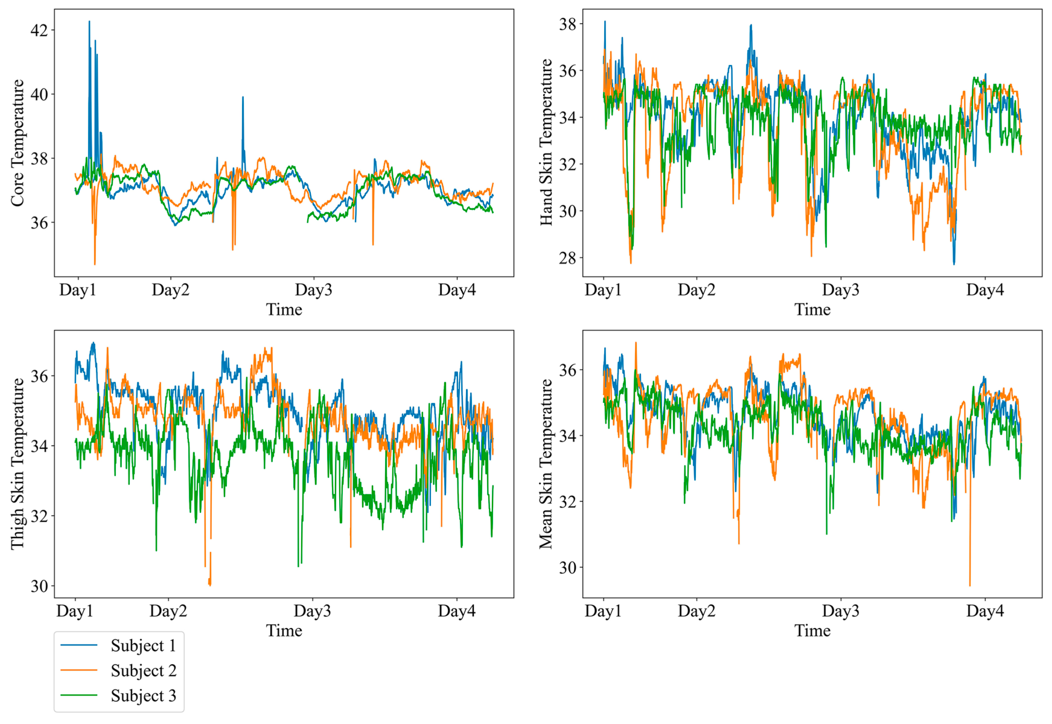
The raw data collected from the experiment are shown in Figure 2.
During the research process, the experimental data were pre-processed before being used for model fine-tuning and testing.
Missing value handling: Inevitably, data collected from the field may have missing values. In this experiment, due to the high cooperation level of the participants, missing values tended to appear in batches rather than being scattered. To address this, during the preprocessing phase, data files containing intervals of missing values were directly split to form multiple internally continuous time-series data files.
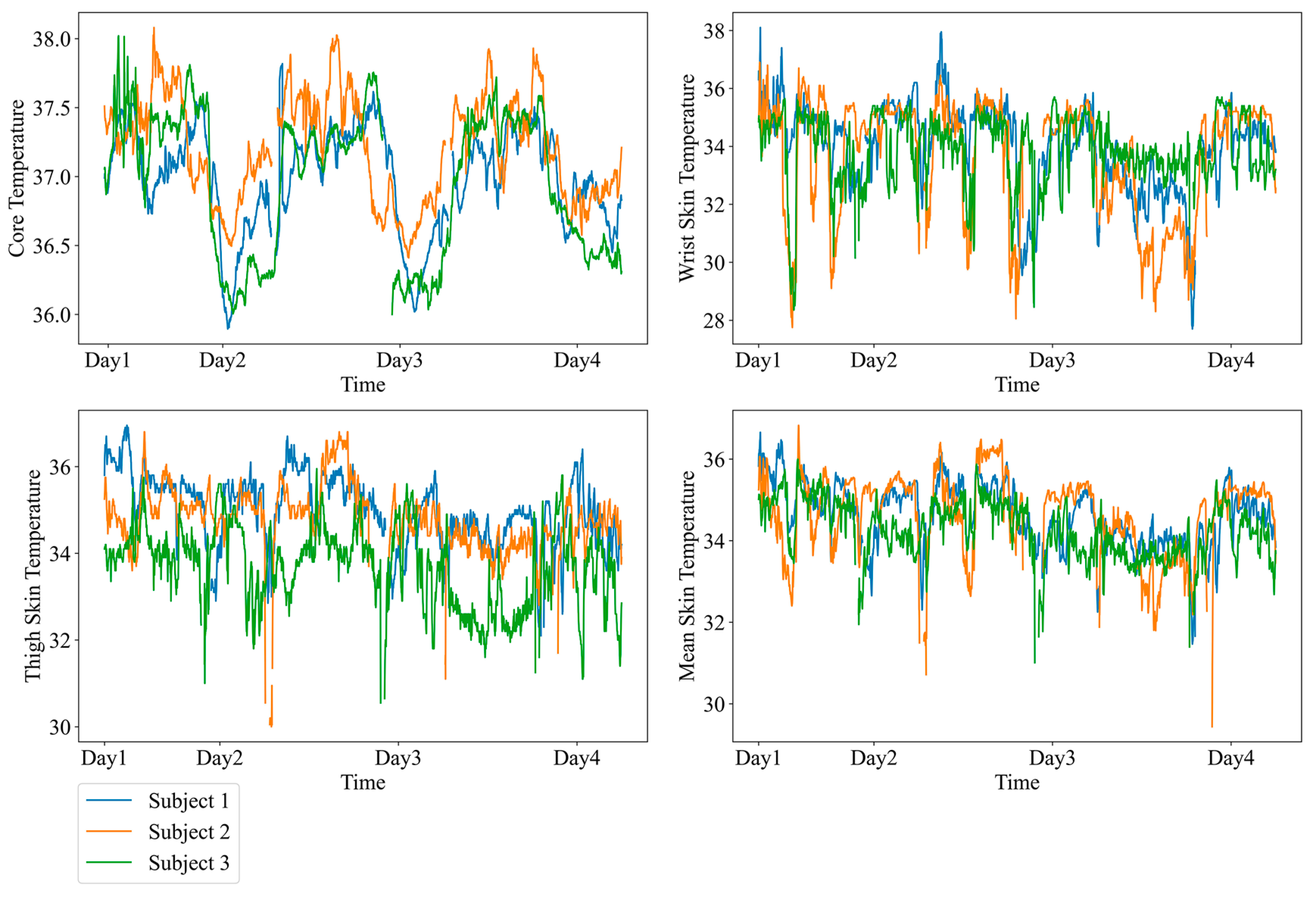
Anomaly handling: Anomalies in Tcr data primarily occurred within the first 4 h after ingesting the capsule. At this time, since the capsule had not fully entered the intestines, activities such as eating and drinking could significantly affect the measurement results from the Tcr capsule. Given that the experiment lasted 72 h, such anomalies were inevitable. However, owing to the active cooperation of the participants, the number of such anomalies was limited, and they did not occur during the work periods of greatest interest to us. These anomalies often appear as sudden waveform changes, making them easy to identify. For these anomalies, the Kalman filter method proposed by Buller [53] was employed to replace the anomalous values, using heart rate measurements to predict Tcr and impute the missing or erroneous values. On the other hand, Tsk data, which are more significantly affected by external factors, exhibited a greater number of anomalies that were not as easily observable. Therefore, Tsk anomalies were not subjected to intervention treatment.
The data, after being processed as described above, are shown in Figure 3.
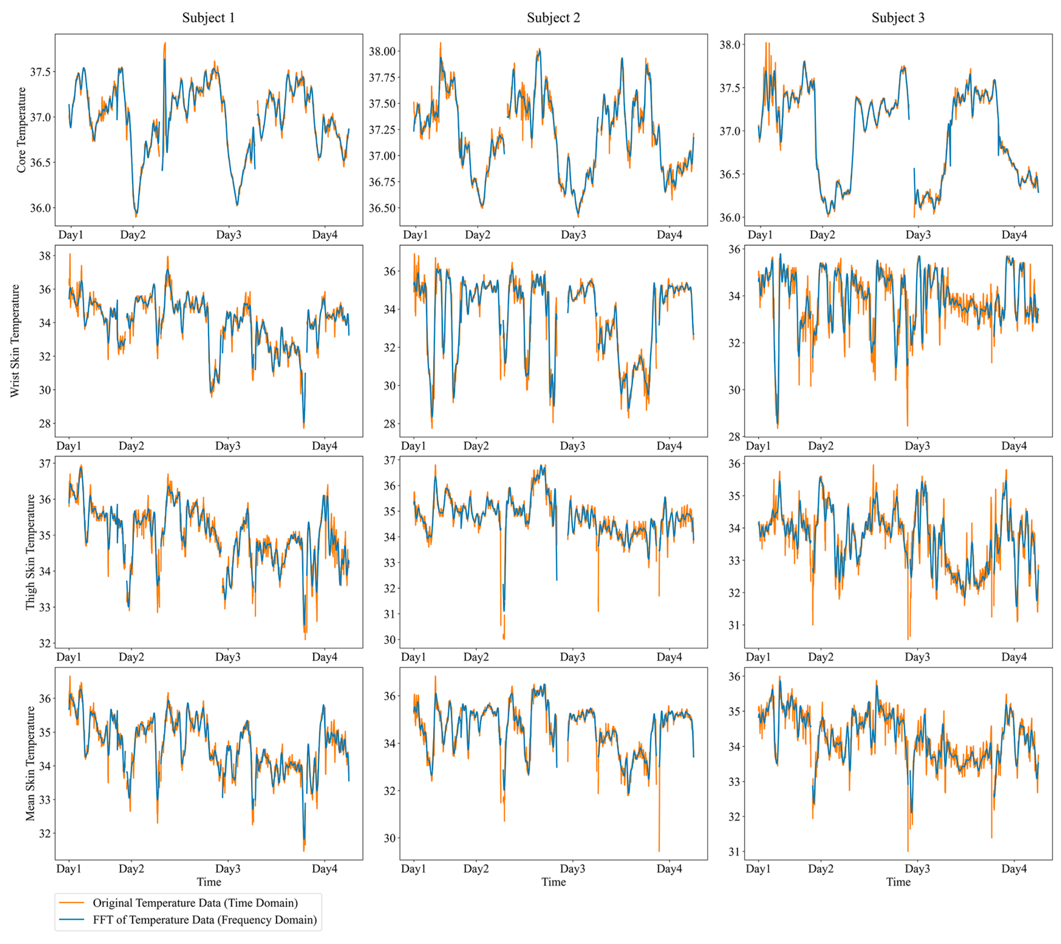
Noise reduction: To better match the granularity of the pretraining data, the fast Fourier-transform (FFT) method was utilized to denoise the experimental data during the research process. Additionally, the cross-correlation function (CCF) was used to examine the predictability and lag characteristics. Finally, for all experimental data, we determined that the required threshold for noise reduction was 0.02, and the threshold was chosen based on a comprehensive evaluation, ensuring that the denoised data exhibited no lag while also minimizing the error when the denoised data were used for model training (Appendix A, Figure A1 and Figure A2). A comparison of the waveforms after noise reduction and the original data is shown in Figure 4.
The aforementioned preprocessing steps aim to ensure that the measured data undergo proper preparation before entering the model training phase to enhance the model’s stability and predictive performance. After the above processing, the remaining available data volume is shown in Table 1.
Dataset split: The training and test sets were constructed in the following manner. For each participant, 720 data points corresponding to the daytime hours (8:00 to 20:00) of the day with the highest experimental temperature were designated the test set, with the remaining data serving as the training set required for TL fine-tuning.

2.2.2. Simulated Dataset

During the data simulation generation phase, the JOS-3 thermo-physiological model was used to generate the simulated data. Throughout the research process, to validate the impact of different pretraining data on the model prediction accuracy, two types of data were simulated, non-personalized generic data and personalized data.
For non-personalized generic data, the simulation process includes two key aspects, personnel simulation and working condition simulation. In the personnel simulation phase, a large number of virtual individuals were simulated, covering age distributions of children, youth, middle-aged individuals, and elderly individuals, including both males and females. The height and weight ranges were restricted within the applicable range for each age and sex group. In the testing process of this study, a total of 180 virtual individuals were simulated, including 90 males and 90 females. The working condition simulation was conducted based on three types of scenarios—daily outdoor, extreme outdoor, and indoor scenarios—with the simulation in hourly units and a cycle lasting 24 h. Different work condition scenarios correspond to variations in temperature, humidity, wind speed, labor intensity level (reflected through the physical activity ratio (PAR)), and human body posture. During the simulation process, the range of all parameters was set based on policies, experience, and common sense. Parameters were randomly selected from their respective parameter ranges for each simulation to obtain results closer to reality. The environmental parameters and labor intensity values corresponding to each level, as well as the level settings for each simulated work condition, are shown in Appendix A, Table A3 and Table A4, respectively. For each virtual individual, one cycle of Tcr and Tsk data was simulated under the three mentioned work condition environments, including data for 21 Tsk points and 17 Tcr points. In total, the number of generic simulated data points reached 777,600. The generic data simulation method can provide simulated Tcr and Tsk data for various virtual individuals and different working conditions, offering broad applicability for diverse application scenarios. This simulation scheme is suitable for application scenarios where the demand for personalization in the pretrained model is relatively low.
For personalized data, virtual human bodies were precisely generated based on actual individual body parameters, and customized work condition environments were created according to their specific work requirements. For the three participants described in the field experiment presented in Section 2.1, three sets of personalized Tcr and Tsk data were constructed. This type of data was simulated based on the specific work condition environments shown in Appendix A, Table A3 (with labor intensity levels and environmental variables levels seen in Appendix A, Table A4 and Table A5). Under the set work condition scenarios, a total of 360 cycles were simulated, resulting in each set of personalized simulation data containing 518,400 entries. This method of generating personalized data can more accurately simulate an individual’s physiological characteristics and work environment, providing greater adaptability and precision for the personalized application of pretrained models. This simulation scheme is suitable for application scenarios that require a high level of personalization in pretrained models.

2.3. Model Training and Testing

The training of the model is divided into two phases, pretraining and fine-tuning. Based on research on on-site conditions, it was determined that the maximum response time workers need after receiving a warning message is 10 min. Therefore, the longest prediction time step was set to 10 (i.e., 10 min). During the pretraining phase, non-personalized generic data and personalized data were utilized to train the generic and personalized models, respectively. The predictive performance of the pretrained models was then evaluated using the generated pretraining test data, and the model hyperparameters were adjusted. Once the pretrained models were fine-tuned to their optimal state, the pretrained model loading module was employed to load the training sets, which were divided from the actual measured data into two types of models for fine-tuning. No further hyperparameter adjustments were made during this phase. Finally, model testing was completed using actual measured test set data.
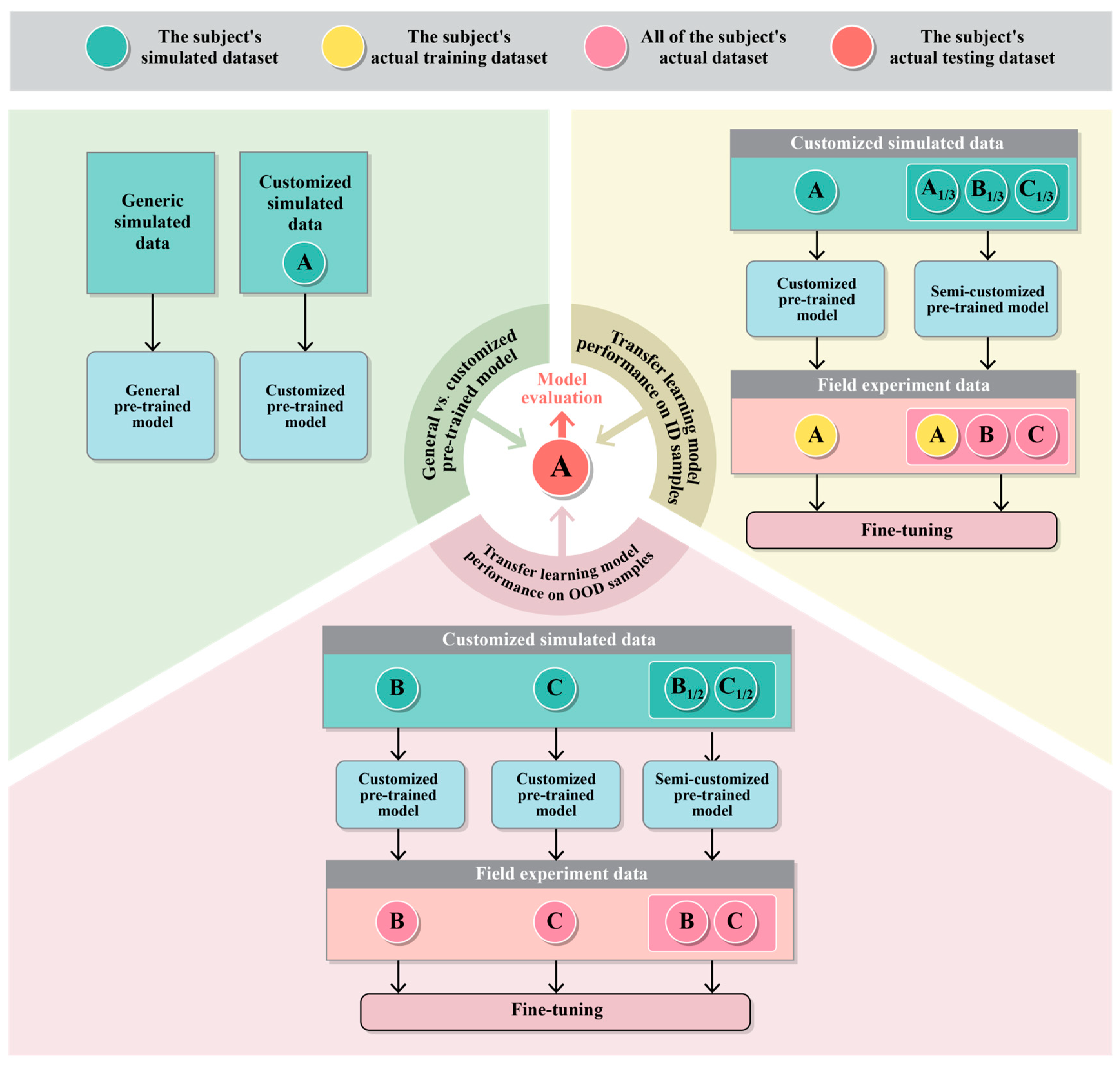
During the final model evaluation, we tested the impact of different training approaches on the model performance. Three main testing methods, as shown in Figure 5 (using data from Participant 1 (A) as an example, with similar approaches applied to other participants), were applied.
Here, A, B, and C represent the datasets of three participants, with the subscript indicating the proportion of data extracted from that dataset. For example, using data from Participant 1 (A), we apply similar approaches to data from the other participants.
Impact of generic simulated data and personalized simulated data on the pretrained model performance: To accomplish this evaluation task, two types of simulated data were generated using the JOS-3 thermo-physiological model, data based on generic simulation and personalized simulated data generated according to the individual body parameters of each participant. These two sets of data were used to pretrain the Informer model separately, and model performance was assessed without undergoing transfer learning. Ultimately, the evaluation results from the three participants were averaged to provide a comprehensive assessment of the model performance.
Predictive performance of the TL model on in-distribution (ID) samples: To complete this task, two tests were conducted, including (1) using simulated data and actual training set data from one participant for model pretraining and transfer learning, followed by model testing and evaluation on the test set data of that participant, and (2) using simulated data from all participants and all actual data except for the test set of the participant to be tested for model pretraining and transfer learning and then conducting model testing and evaluation on the reserved test set. Finally, the evaluation results from the three participants were averaged to complete a comprehensive assessment of the model performance.
Predictive performance of the transfer learning model on out-of-distribution (OOD) samples: To complete this evaluation task, two tests were conducted, including (1) using simulated data from two participants and all actual data for model pretraining and transfer learning, followed by separate model testing and evaluation on the test set data of the third participant, with the results averaged; and (2) using simulated data from two participants and all actual data for model pretraining and transfer learning and then conducting model testing and evaluation on the test set data of the third participant. Finally, the evaluation results from the three participants were averaged to complete a comprehensive assessment of the model performance.

3. Results

Given that the aim of the prediction task is to determine the Tcr and Tsk ten minutes later, in the least ideal prediction scenario, the model will not make any predictions and will directly output the most recent observation data as the prediction value, resulting in the model predictions lagging by ten minutes. To conduct a comparative evaluation, the observed values in the test set were shifted backwards by ten minutes to serve as the prediction values for the control group. By evaluating the performance of the control group prediction values, a benchmark metric can be established to compare and assess against the model prediction results. The evaluation results for each training method model are shown in Table 2, Table 3 and Table 4. It should be noted that all the following results are compared against data collected by sensors, and the inherent errors of the sensors themselves have not been taken into consideration.
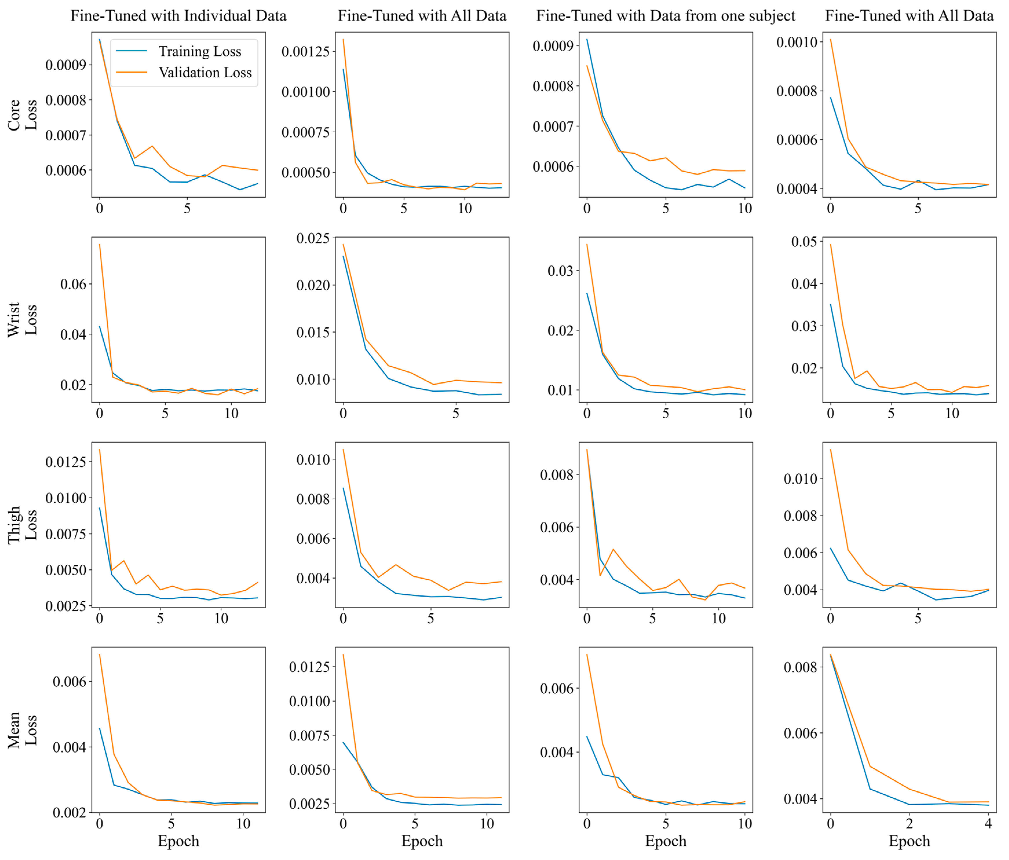
From the three tables above, it is evident that regardless of the prediction method used, the prediction results are superior to those of the ten-minute lag control group, indicating the effectiveness of the model predictions. Based on the evaluation results observed on the training and test datasets, the model fits the data well, with no obvious signs of overfitting or underfitting. The model’s learning curve and validation loss further support this conclusion, demonstrating consistent performance throughout the training process (Appendix A, Figure A3).
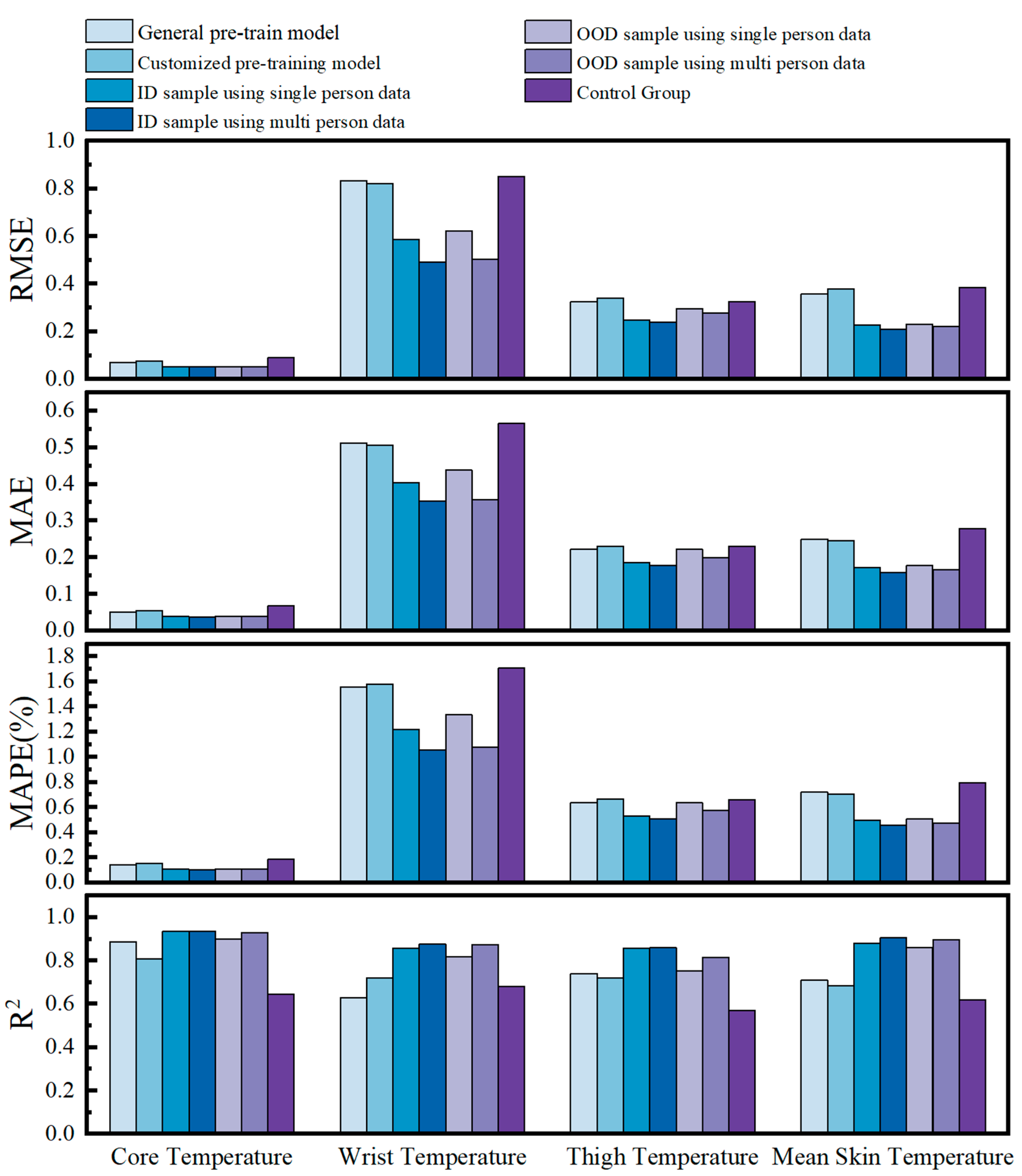
As shown in Table 2, when predictions are made using only the pretrained model, the results are only slightly better than those of the ten-minute lag control group, indicating that without model transfer, the predictions made using only the pretrained model cannot meet practical needs. Additionally, comparing the generic model with the customized model, whether for the Tcr or Tsk, the predictive performance of the customized model is superior to that of the generic model.
Based on Table 3 and Table 4, for both the ID and OOD samples, the model performance significantly improves after TL. When the data volume is roughly consistent, the model prediction accuracy on the ID data slightly surpasses that on the OOD data. However, as the volume of data involved in TL increases, the model prediction accuracy further increases. When there are more OOD data, the accuracy of the fine-tuned transfer model can even surpass that of models fine-tuned with a smaller amount of ID data. In particular, when using all training data for TL, the larger the volume of data involved in transfer learning is, particularly for ID learning, the better the predictive performance. This finding indicates that the volume of data involved in transfer learning has not yet reached the model’s learning capacity limit. As the data volume continues to increase, the model is expected to achieve an even better performance.
A comparison of the evaluation results above is shown in Figure 6.
For all TL models, as the number of anomalies in the actual data gradually increases, the predictive performance of the models is more significantly affected. For instance, in the current optimal model with a larger volume of ID samples, the Tcr data, influenced by the collection method and having undergone anomaly handling, contain the lowest number of anomalies. In such cases, the prediction error is only 0.04 °C. However, for the Thand data, which are most affected by external conditions and contain the highest number of anomalies, the prediction error is close to 0.4 °C.
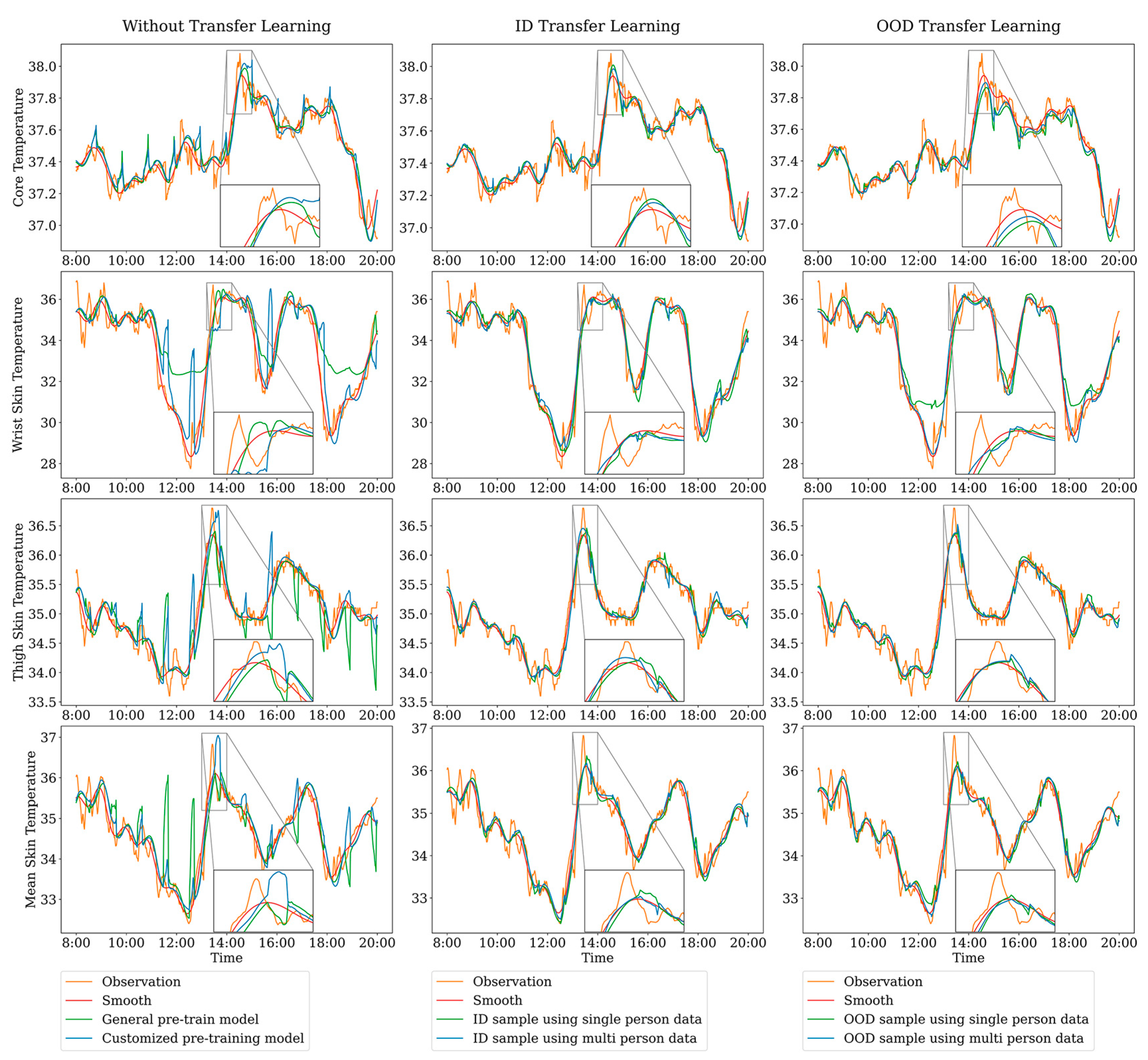
A comparison of the prediction results for the various prediction methods (using Participant 2 as an example) is shown in Figure 7.
According to Figure 7, when TL is not conducted, the model prediction results exhibit a certain degree of lag and abnormal fluctuations, rendering them unsuitable for practical forecasting. However, after implementing TL, the model’s predictive performance is significantly enhanced, with lag and abnormal fluctuations substantially mitigated. When the data volume for TL is consistent, ID predictions are significantly better than OOD predictions, especially for individual-specific fluctuation types. When the data volume for TL is inconsistent, an increase in data volume plays a more significant role; the greater the data volume is, the closer the prediction waveform is to the denoised waveform.
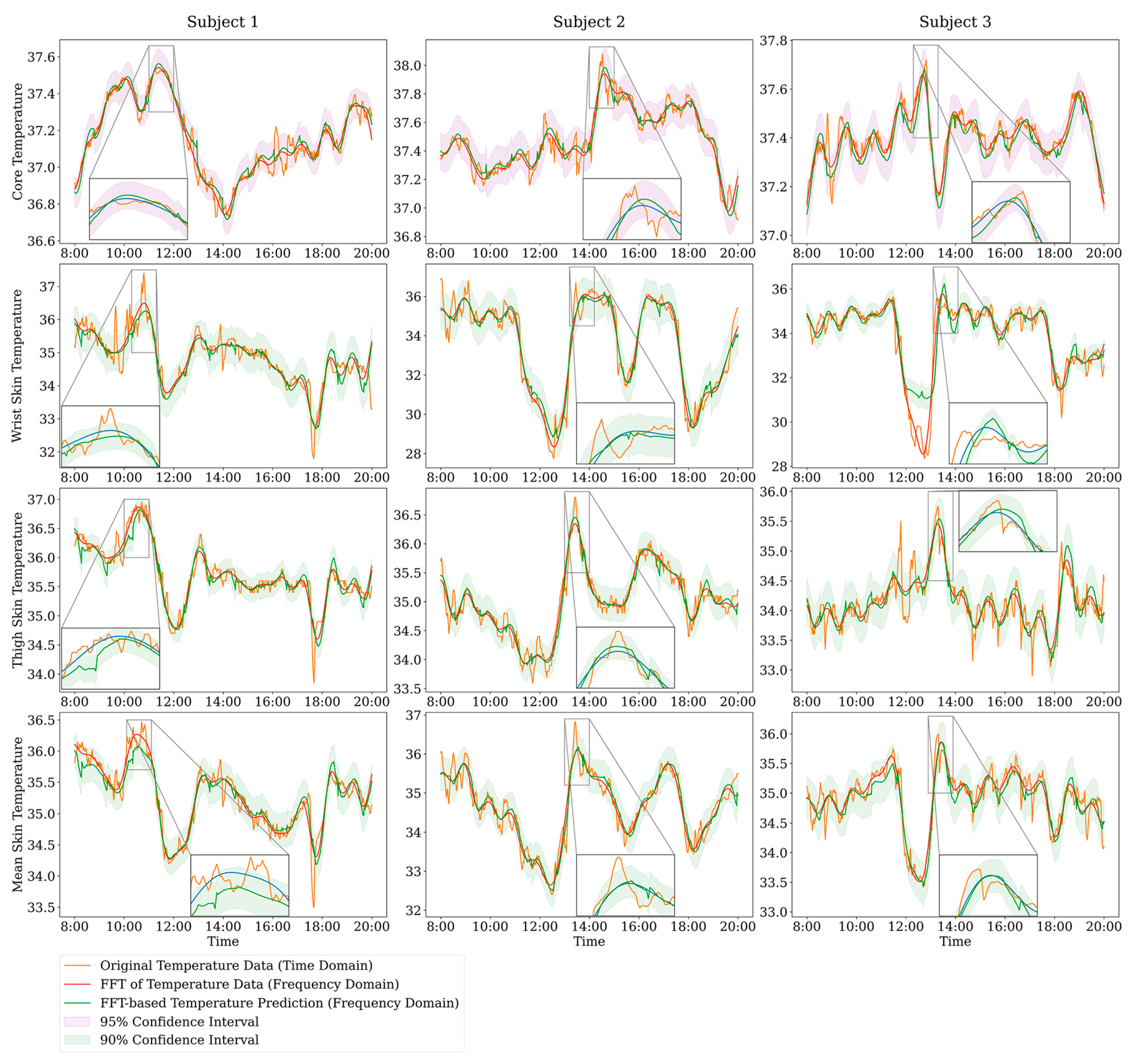
Additionally, in practical applications, due to the denoising process that actual data undergo during the preprocessing stage, the model prediction results inevitably contain errors. Therefore, sufficient guidance cannot be obtained using prediction results as the sole reference. Thus, confidence intervals were introduced to offer more reliable guidance. In this research, a 95% confidence interval was used as a basis for guidance for Tcr, which exhibits smaller noise fluctuations. For Tsk, which exhibits larger noise fluctuations, a 90% confidence interval was used as the reference range. The confidence intervals were calculated using a five-fold cross-validation approach, ensuring a more robust estimation of model performance. In the best-performing prediction results (i.e., predictions made using a customized pretrained model combined with all data and employing ID for TL), confidence intervals were calculated. The specific calculation results are shown in Table 5, and a comparison of the prediction results is shown in Figure 8.
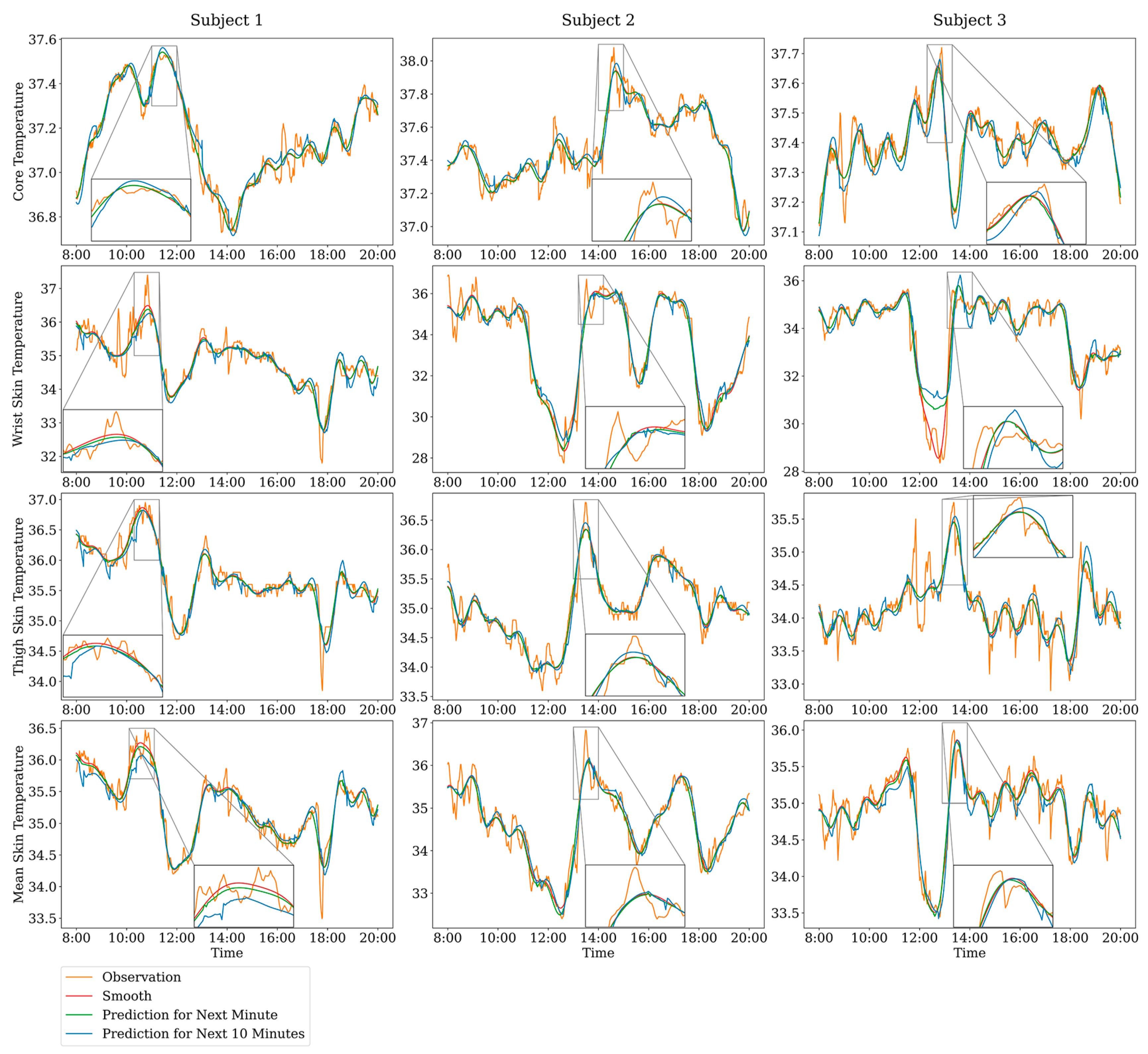
As shown in Figure 8, none of the prediction results exhibit a noticeable lag. Moreover, under high-temperature conditions, the model successfully predicts the temperature trends accurately. However, in cases of rapid temperature changes, due to the noise loss in the data waveforms after denoising, the model cannot perfectly fit the actual data.
Notably, as a long-term forecasting model, the proposed model is not only capable of predicting Tcr and Tsk ten minutes ahead but is also able to make predictions for each minute from the first to the tenth minute. Moreover, the closer to the current moment the prediction time is, the more accurate the prediction result tends to be. For example, Figure 9 shows a comparison between the prediction results one minute ahead and ten minutes ahead.

4. Discussion

According to the results above, after sufficient pretraining with a large volume of simulated data, the proposed model is capable of achieving accurate predictions through TL training with just over 3000 actual data points. In practical use, the model can also adjust its training and application modes according to real-world conditions. When a user’s personal information is known and sufficient data are collected for TL training, the trained model can undoubtedly achieve optimal accuracy. However, if the collected data volume is insufficient for fine-tuning, incorporating data from other individuals can improve the accuracy to a certain extent. If the user is unknown, by simply using existing data for training and fine-tuning, the model can still provide relatively accurate predictions. This discovery undoubtedly significantly expands the application range of the model.
Without subsequent TL of the model and solely using simulated data for training, it is possible to make predictions with a certain level of accuracy. Although these predictions contain a number of anomalies and exhibit slight lags, the overall trend is still reported.
This finding indicates that the model can grasp the physical laws within the human thermo-physiological model and accurately apply these laws in predicting actual data, although this generalized physical law does not provide the best predictive effect. However, when a small portion of the actual data are added for fine-tuning, the model quickly corrects its errors, eliminates anomalous predictions and lag in the prediction results, and makes accurate predictions. The accuracy of these results varies with the number of anomalies in the actual data. For Tcr, the environment during data collection is the most stable, and since anomaly handling is performed in advance, the prediction accuracy is the highest (with a deviation of approximately 0.04 °C). In contrast, for the Thand, which is most affected by external factors during data collection and has not undergone anomaly handling, the prediction accuracy is the lowest (with a deviation of approximately 0.4 °C).
Additionally, as a long-term forecasting model, the model provides accurate predictions for any minute within a ten-minute timeframe, undoubtedly offering more usable information for assisting in the thermal strain warning process. It is foreseeable that this model also has the potential to make predictions for periods longer than ten minutes, even though it has not been extensively tested for such capabilities.
However, this study has several limitations. First, the amount of data used in the model fine-tuning process does not meet the training needs of the model, leading to underfitting. Second, the number of participants involved in the model testing process is limited, and their characteristics are relatively homogeneous. Therefore, the model’s effectiveness across different types of populations has not been fully tested. Third, the original study [41] does not provide a detailed validation of boundary conditions, which are critical for the numerical method’s robustness. This limitation has been acknowledged in the present study, and we emphasize that the model was applied based on its validation in previous work. Nevertheless, further research should address the model’s boundary conditions to enhance its stability and accuracy in diverse applications. Finally, due to the high degree of information loss from current real-time noise reduction methods, the data denoising method used in this study is not real-time. These issues will be addressed in future research.

5. Conclusions

This study provides a novel prediction method for Tcr and Tsk. By utilizing data from a continuous 72 h field experiment along with JOS-3 model-simulated data, combined with LTSF and TL methods, we developed a real-time prediction model for Tcr and Tsk. The model has the following characteristics: (a) It operates independently of environmental, human, and clothing parameters. It utilizes over 3000 historically collected real temperature data points for training. During prediction, it only requires the temperature data from the past 25 min to personalize predictions of Tcr and Tsk within the next 10 min. (b) It achieves accurate real-time predictions of Tcr and Tsk within the next 10 min, with a prediction error for Tcr within ±0.14 °C (95% confidence interval), for Tsk,mean within ±0.46 °C (90% confidence interval), and for all local Tsk within ±0.97 °C, with the prediction error for Tthigh reaching ±0.36 °C. This high-precision prediction provides sufficient warning response time for workers in high-temperature environments, helping them take timely measures to avoid the risk of heat-related injuries.

Author Contributions

X.H.: Conceptualization, Methodology, Writing—Original Draft, Visualization. J.W.: Formal Analysis, Validation, Funding Acquisition, Data Curation, Supervision. Z.H.: Writing—Reviewing and Editing, Methodology, Investigation. C.L.: Formal Analysis, Visualization, Project Administration. B.S.: Validation, Formal Analysis. All authors have read and agreed to the published version of the manuscript.

Funding

This research was funded by the Ordos Key Research and Development Program, grant number YF20232304.

Institutional Review Board Statement

This study was conducted in accordance with the Declaration of Helsinki, and approved by the Scientific Research Ethics Committee of China University of Mining and Technology (Beijing).

Informed Consent Statement

Informed consent was obtained from all subjects involved in this study.

Data Availability Statement

The data presented in this study are available on request from the corresponding author due to the data also forming part of an ongoing study.

Conflicts of Interest

The authors declare no conflict of interest.

Appendix A

Table A1. Hyperparameter settings for the Informer model.
HyperparameterValue
Prediction TaskUnivariate Forecasting Univariate
Max Epoch20
Patience3
Activation FunctionGELU
Initial Learning Rate0.00001
Dropout Rate0.05
Loss FunctionMean Squared Error (MSE)
Token LengthSame as Prediction Sequence Length
Input Sequence LengthTwice the Prediction Sequence Length
Attention Sampling Number5
Model Dimension512
Number of Heads in Multi-Head Attention8
Number of Encoder Layers2
Number of Decoder Layers1
Table A2. Basic information of subjects.
Subject IDAgeHeight (m)Weight (kg)Work Environment
1511.765Semi-indoor/Semi-outdoor
2611.6861Outdoor
3331.7273Indoor
Table A3. Environmental variable levels for personalized simulated environments.
SubjectsTime (h)Temperature LevelHumidity LevelWind Speed LevelLabor Intensity LevelPosture
Subject 10–71200Lying
7–8220/10Standing
8–102/3101/2Standing
10–122/3/4101/2Standing
12–131100Sitting
13–141101/2Sitting
14–172/3/4101/2Standing
17–182/3101/2Standing
18–191/2101/2Sitting
19–202/3101/2Standing
20–212/310/11/2Standing
21–241100Sitting
Subject 20–71200Lying
7–8220/11/2Standing
8–102/3101/2Standing
10–122/3/4101/2Standing
12–13110/10Sitting
13–14110/11/2Sitting
14–172/3/410/11/2Standing
17–182/310/11/2Standing
18–191/210/10/1Sitting
19–211/210/10Sitting
21–241100Lying
Subject 30–71200Lying
7–81/2200Standing
8–101/2101/2Standing
10–122101/2Standing
12–131100Sitting
13–141101/2Sitting
14–172/3101/2Standing
17–181/2101/2Standing
18–191101/2Sitting
19–201/2101/2Standing
20–211/2101/2Standing
21–241100Sitting
Table A4. Environmental and labor intensity parameter ranges by level.
ParametersLevelRange
Air Temperature023–26 (°C)
127–30 (°C)
231–33 (°C)
334–37 (°C)
438–42(°C)
Air Humidity00–30 (%)
131–60 (%)
261–95 (%)
Wind Speed00–1.5 (m/s)
11.6–3.3 (m/s)
23.4–5.4 (m/s)
35.5–7.9 (m/s)
48.0–10.7 (m/s)
PAR [54]01–2.5
12.6–3.9
24.0–7.0
Table A5. Environmental variable levels for each simulated environment.
Simulated EnvironmentTime (h)Temperature LevelHumidity LevelWind Speed LevelLabor Intensity LevelPosture
Daily Outdoor Work 0–70100Lying
7–90100Sitting
9–101232Standing
10–122222Standing
12–131100Sitting
13–163211Standing
16–182232Standing
18–202121Sitting
20–240100Sitting
Extreme Outdoor Work0–70100Lying
7–90100Sitting
9–102232Standing
10–123242Standing
12–131100Sitting
13–164211Standing
16–183232Standing
18–202121Sitting
20–240100Sitting
Indoor Work0–70100Lying
7–90100Sitting
9–101202Sitting
10–121202Sitting
12–132100Sitting
13–161201Sitting
16–181202Sitting
18–202101Sitting
20–240100Sitting
Figure A1. FFT threshold evaluation of Tcr.
Bdcc 08 00197 g0a1
Figure A2. FFT threshold evaluation of Tsk.
Bdcc 08 00197 g0a2
Figure A3. The model’s learning curve and validation loss.
Bdcc 08 00197 g0a3

References

  1. Heikens, M.J.; Gorbach, A.M.; Eden, H.S.; Savastano, D.M.; Chen, K.Y.; Skarulis, M.C.; Yanovski, J.A. Core Body Temperature in Obesity. Am. J. Clin. Nutr. 2011, 93, 963–967. [Google Scholar] [CrossRef] [PubMed]
  2. Pascoe, D.D.; Mercer, J.B.; de Weerd, L. Physiology of Thermal Signals. In Medical Devices and Systems; CRC Press: Boca Raton, FL, USA, 2006; pp. 447–466. ISBN 0429123043. [Google Scholar]
  3. Joshi, A.; Wang, F.; Kang, Z.; Yang, B.; Zhao, D. A Three-Dimensional Thermoregulatory Model for Predicting Human Thermophysiological Responses in Various Thermal Environments. Build. Environ. 2022, 207, 108506. [Google Scholar] [CrossRef]
  4. Fiala, D.; Lomas, K.J.; Stohrer, M. Computer Prediction of Human Thermoregulatory and Temperature Responses to a Wide Range of Environmental Conditions. Int. J. Biometeorol. 2001, 45, 143–159. [Google Scholar] [CrossRef] [PubMed]
  5. Tanabe, S.; Kobayashi, K.; Nakano, J.; Ozeki, Y.; Konishi, M. Evaluation of Thermal Comfort Using Combined Multi-Node Thermoregulation (65MN) and Radiation Models and Computational Fluid Dynamics (CFD). Energy Build. 2002, 34, 637–646. [Google Scholar] [CrossRef]
  6. Kobayashi, Y.; Tanabe, S. Development of JOS-2 Human Thermoregulation Model with Detailed Vascular System. Build. Environ. 2013, 66, 1–10. [Google Scholar] [CrossRef]
  7. Huizenga, C.; Hui, Z.; Arens, E. A Model of Human Physiology and Comfort for Assessing Complex Thermal Environments. Build. Environ. 2001, 36, 691–699. [Google Scholar] [CrossRef]
  8. Gulati, T.; Hatwar, R.; Unnikrishnan, G.; Rubio, J.E.; Reifman, J. A 3-D Virtual Human Model for Simulating Heat and Cold Stress. J. Appl. Physiol. 2022, 133, 288–310. [Google Scholar] [CrossRef] [PubMed]
  9. Unnikrishnan, G.; Hatwar, R.; Hornby, S.; Laxminarayan, S.; Gulati, T.; Belval, L.N.; Giersch, G.E.W.; Kazman, J.B.; Casa, D.J.; Reifman, J. A 3-D Virtual Human Thermoregulatory Model to Predict Whole-Body and Organ-Specific Heat-Stress Responses. Eur. J. Appl. Physiol. 2021, 121, 2543–2562. [Google Scholar] [CrossRef]
  10. Wu, Z.; Yang, R.; Qian, X.; Yang, L.; Lin, M. A Multi-Segmented Human Bioheat Model under Immersed Conditions. Int. J. Therm. Sci. 2023, 185, 108029. [Google Scholar] [CrossRef]
  11. Salloum, M.; Ghaddar, N.; Ghali, K. A New Transient Bioheat Model of the Human Body and Its Integration to Clothing Models. Int. J. Therm. Sci. 2007, 46, 371–384. [Google Scholar] [CrossRef]
  12. Younes, J.; Chen, M.; Ghali, K.; Kosonen, R.; Melikov, A.K.; Ghaddar, N. A Thermal Sensation Model for Elderly under Steady and Transient Uniform Conditions. Build. Environ. 2023, 227, 109797. [Google Scholar] [CrossRef]
  13. Davoodi, F.; Hassanzadeh, H.; Zolfaghari, S.A.; Havenith, G.; Maerefat, M. A New Individualized Thermoregulatory Bio-Heat Model for Evaluating the Effects of Personal Characteristics on Human Body Thermal Response. Build. Environ. 2018, 136, 62–76. [Google Scholar] [CrossRef]
  14. Fu, M.; Weng, W.; Chen, W.; Luo, N. Review on Modeling Heat Transfer and Thermoregulatory Responses in Human Body. J. Therm. Biol. 2016, 62, 189–200. [Google Scholar] [CrossRef] [PubMed]
  15. Petersson, J.; Kuklane, K.; Gao, C. Is There a Need to Integrate Human Thermal Models with Weather Forecasts to Predict Thermal Stress? Int. J. Environ. Res. Public. Health 2019, 16, 4586. [Google Scholar] [CrossRef]
  16. Makhlouf, K.; Hmidi, Z.; Kahloul, L.; Benhrazallah, S.; Ababsa, T. On the Forecasting of Body Temperature Using Iot and Machine Learning Techniques. In Proceedings of the 2021 International Conference on Theoretical and Applicative Aspects of Computer Science (ICTAACS), Skikda, Algeria, 15–16 December 2021; pp. 1–6. [Google Scholar]
  17. Staffini, A.; Svensson, T.; Chung, U.; Svensson, A.K. Heart Rate Modeling and Prediction Using Autoregressive Models and Deep Learning. Sensors 2021, 22, 34. [Google Scholar] [CrossRef] [PubMed]
  18. Nazarian, N.; Liu, S.; Kohler, M.; Lee, J.K.W.; Miller, C.; Chow, W.T.L.; Alhadad, S.B.; Martilli, A.; Quintana, M.; Sunden, L. Project Coolbit: Can Your Watch Predict Heat Stress and Thermal Comfort Sensation? Environ. Res. Lett. 2021, 16, 034031. [Google Scholar] [CrossRef]
  19. Boudreault, J.; Campagna, C.; Chebana, F. Machine and Deep Learning for Modelling Heat-Health Relationships. Sci. Total Environ. 2023, 892, 164660. [Google Scholar] [CrossRef] [PubMed]
  20. Dasari, A.; Revanur, A.; Jeni, L.A.; Tucker, C.S. Video-Based Elevated Skin Temperature Detection. IEEE Trans. Biomed. Eng. 2023, 70, 2430–2444. [Google Scholar] [CrossRef] [PubMed]
  21. Carluccio, G.; Erricolo, D.; Oh, S.; Collins, C.M. An Approach to Rapid Calculation of Temperature Change in Tissue Using Spatial Filters to Approximate Effects of Thermal Conduction. IEEE Trans. Biomed. Eng. 2013, 60, 1735–1741. [Google Scholar] [CrossRef]
  22. Zhong, W.; Mallick, T.; Meidani, H.; Macfarlane, J.; Balaprakash, P. Explainable Graph Pyramid Autoformer for Long-Term Traffic Forecasting. arXiv 2022, arXiv:2209.13123. [Google Scholar] [CrossRef]
  23. Pan, G.; Wu, Q.; Ding, G.; Wang, W.; Li, J.; Zhou, B. An Autoformer-CSA Approach for Long-Term Spectrum Prediction. IEEE Wirel. Commun. Lett. 2023, 12, 1647–1651. [Google Scholar] [CrossRef]
  24. Jiang, Y.; Gao, T.; Dai, Y.; Si, R.; Hao, J.; Zhang, J.; Gao, D.W. Very Short-Term Residential Load Forecasting Based on Deep-Autoformer. Appl. Energy 2022, 328, 120120. [Google Scholar] [CrossRef]
  25. Gong, M.; Zhao, Y.; Sun, J.; Han, C.; Sun, G.; Yan, B. Load Forecasting of District Heating System Based on Informer. Energy 2022, 253, 124179. [Google Scholar] [CrossRef]
  26. Yang, Z.; Liu, L.; Li, N.; Tian, J. Time Series Forecasting of Motor Bearing Vibration Based on Informer. Sensors 2022, 22, 5858. [Google Scholar] [CrossRef]
  27. Wang, C.; Mahadevan, S. Heterogeneous Domain Adaptation Using Manifold Alignment. IJCAI Proc.-Int. Jt. Conf. Artif. Intell. 2011, 22, 1541. [Google Scholar]
  28. Duan, L.; Xu, D.; Tsang, I. Learning with Augmented Features for Heterogeneous Domain Adaptation. arXiv 2012, arXiv:1206.4660. [Google Scholar] [CrossRef]
  29. Kulis, B.; Saenko, K.; Darrell, T. What You Saw Is Not What You Get: Domain Adaptation Using Asymmetric Kernel Transforms. In Proceedings of the CVPR 2011, Colorado Springs, CO, USA, 20–25 June 2011; pp. 1785–1792. [Google Scholar]
  30. Zhu, Y.; Chen, Y.; Lu, Z.; Pan, S.; Xue, G.-R.; Yu, Y.; Yang, Q. Heterogeneous Transfer Learning for Image Classification. AAAI Conf. Artif. Intell. 2011, 25, 1304–1309. [Google Scholar] [CrossRef]
  31. Radočaj, P.; Radočaj, D.; Martinović, G. Image-Based Leaf Disease Recognition Using Transfer Deep Learning with a Novel Versatile Optimization Module. Big Data Cogn. Comput. 2024, 8, 52. [Google Scholar] [CrossRef]
  32. Harel, M.; Mannor, S. Learning from Multiple Outlooks. arXiv 2010, arXiv:1005.0027. [Google Scholar] [CrossRef]
  33. Shu, Z.; Zhou, Y.; Zhang, J.; Jin, J.; Wang, L.; Cui, N.; Wang, G.; Zhang, J.; Wu, H.; Wu, Z.; et al. Parameter Regionalization Based on Machine Learning Optimizes the Estimation of Reference Evapotranspiration in Data Deficient Area. Sci. Total Environ. 2022, 844, 157034. [Google Scholar] [CrossRef]
  34. Nam, J.; Kim, S. Heterogeneous Defect Prediction. In Proceedings of the 2015 10th Joint Meeting on Foundations of Software Engineering, Bergamo Italy, 30 August–4 September 2015; pp. 508–519. [Google Scholar]
  35. Zhang, W.; Wang, Z.; Li, X. Blockchain-Based Decentralized Federated Transfer Learning Methodology for Collaborative Machinery Fault Diagnosis. Reliab. Eng. Syst. Saf. 2023, 229, 108885. [Google Scholar] [CrossRef]
  36. Mao, W.; Zhang, W.; Feng, K.; Beer, M.; Yang, C. Tensor Representation-Based Transferability Analytics and Selective Transfer Learning of Prognostic Knowledge for Remaining Useful Life Prediction across Machines. Reliab. Eng. Syst. Saf. 2024, 242, 109695. [Google Scholar] [CrossRef]
  37. Abdelhamid, S.; Hegazy, I.; Aref, M.; Roushdy, M. Attention-Driven Transfer Learning Model for Improved IoT Intrusion Detection. Big Data Cogn. Comput. 2024, 8, 116. [Google Scholar] [CrossRef]
  38. Prettenhofer, P.; Stein, B. Cross-Language Text Classification Using Structural Correspondence Learning. In Proceedings of the 48th Annual Meeting of the Association for Computational Linguistics, Uppsala, Sweden, 11–16 July 2010; pp. 1118–1127. [Google Scholar]
  39. Zhou, J.T.; Tsang, I.W.; Pan, S.J.; Tan, M. Heterogeneous Domain Adaptation for Multiple Classes. Artif. Intell. Stat. PMLR 2014, 33, 1095–1103. [Google Scholar]
  40. Zhou, J.; Pan, S.; Tsang, I.; Yan, Y. Hybrid Heterogeneous Transfer Learning through Deep Learning. AAAI Conf. Artif. Intell. 2014, 28, 2213–2219. [Google Scholar] [CrossRef]
  41. Takahashi, Y.; Nomoto, A.; Yoda, S.; Hisayama, R.; Ogata, M.; Ozeki, Y.; Tanabe, S. Thermoregulation Model JOS-3 with New Open Source Code. Energy Build. 2021, 231, 110575. [Google Scholar] [CrossRef]
  42. Stolwijk, J.A.J. A Mathematical Model of Physiological Temperature Regulation in Man; NASA, Yale University: New Haven, CT, USA, 1971. [Google Scholar]
  43. Oyama, T.; Fujii, M.; Nakajima, K.; Takakura, J.; Hijioka, Y. Validation of Upper Thermal Thresholds for Outdoor Sports Using Thermal Physiology Modelling. Temperature 2023, 11, 92–106. [Google Scholar] [CrossRef]
  44. Choudhary, B. Udayraj Validity of the JOS-3 Model for Male Tropical Population and Analysis of Their Thermal Comfort. Sādhanā 2023, 48, 208. [Google Scholar] [CrossRef]
  45. Jia, X.; Li, S.; Zhu, Y.; Ji, W.; Cao, B. Transient Thermal Comfort and Physiological Responses Following a Step Change in Activity Status under Summer Indoor Environments. Energy Build. 2023, 285, 112918. [Google Scholar] [CrossRef]
  46. Liang, H.; Tanabe, S.; Niu, J. Coupled Simulation of CFD and Human Thermoregulation Model in Outdoor Wind Environment. E3S Web Conf. 2023, 396, 05008. [Google Scholar] [CrossRef]
  47. d’Ambrosio Alfano, F.R.; Palella, B.I.; Riccio, G. THERMODE 2023: Formulation and Validation of a New Thermo-Physiological Model for Moderate Environments. Build. Environ. 2024, 252, 111272. [Google Scholar] [CrossRef]
  48. Choudhary, B. A Coupled CFD-Thermoregulation Model for Air Ventilation Clothing. Energy Build. 2022, 268, 112206. [Google Scholar] [CrossRef]
  49. Zhou, H.; Zhang, S.; Peng, J.; Zhang, S.; Li, J.; Xiong, H.; Zhang, W. Informer: Beyond Efficient Transformer for Long Sequence Time-Series Forecasting. AAAI Conf. Artif. Intell. 2021, 35, 11106–11115. [Google Scholar] [CrossRef]
  50. Wang, G.; Bai, H. Study on the Climate Changes in Cangzhou in Recent 38 Years. Meteorol. Environ. Res. 2012, 3, 16–17+23. [Google Scholar]
  51. Service, T.W.; Junker, K.; Service, B.; Coehoorn, C.J.; Harrington, M.; Martin, S.; Stuart-Hill, L.A. An Assessment of the Validity and Reliability of the P022–P Version of e-Celsius Core Temperature Capsules. J. Therm. Biol. 2023, 112, 103486. [Google Scholar] [CrossRef] [PubMed]
  52. Hardy, J.D.; Du Bois, E.F.; Soderstrom, G.F. The Technic of Measuring Radiation and Convection: One Figure. J. Nutr. 1938, 15, 461–475. [Google Scholar] [CrossRef]
  53. Buller, M.J.; Tharion, W.J.; Cheuvront, S.N.; Montain, S.J.; Kenefick, R.W.; Castellani, J.; Latzka, W.A.; Roberts, W.S.; Richter, M.; Jenkins, O.C. Estimation of Human Core Temperature from Sequential Heart Rate Observations. Physiol. Meas. 2013, 34, 781. [Google Scholar] [CrossRef] [PubMed]
  54. Joint FAO/WHO/UNU. Human Energy Requirements: Report of a Joint FAO/WHO/UNU Expert Consultation, Rome, 17–24 October 2001; UNU/WHO/FAO: Rome, Italy, 2004. [Google Scholar]
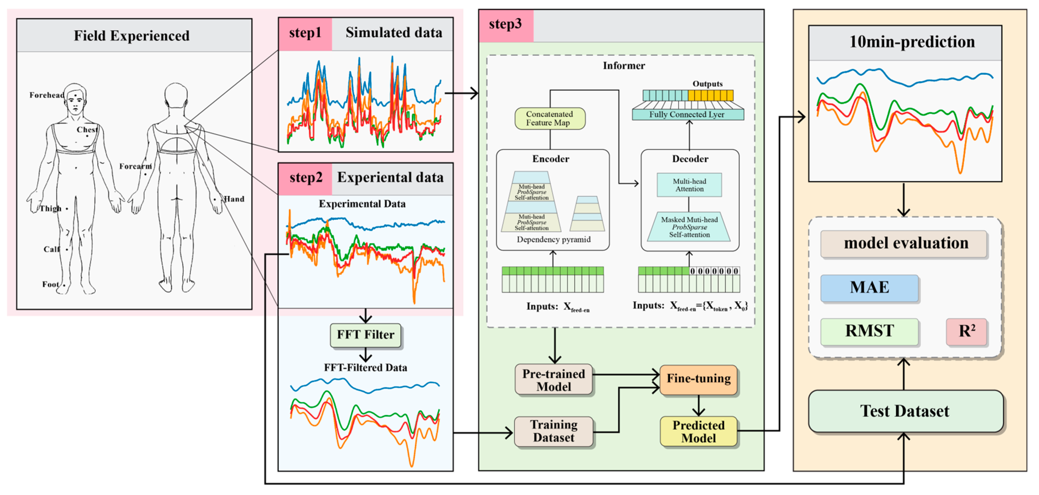
Figure 1. Methodological framework.
Bdcc 08 00197 g001
Figure 2. Raw temperature waveform graphs of various body parts of the participants.
Bdcc 08 00197 g002
Figure 3. Temperature waveform graphs of various body parts of the participants after handling missing and anomalous values.
Bdcc 08 00197 g003
Figure 4. Temperature waveform graphs of various body parts of the participants after noise reduction and the original data.
Bdcc 08 00197 g004
Figure 5. Architecture diagram of the model training and testing evaluation methods.
Bdcc 08 00197 g005
Figure 6. Comparison chart of the model evaluation results.
Bdcc 08 00197 g006
Figure 7. Comparison chart of the prediction results by different model training methods.
Bdcc 08 00197 g007
Figure 8. Comparison chart of the model prediction results including confidence intervals.
Bdcc 08 00197 g008
Figure 9. Comparison of the model predictions 1 minute and 10 minutes into the future.
Bdcc 08 00197 g009
Table 1. Available data volume of the measured data.
Participant IDAmount of Tcr DataAmount of Tsk Data
141684108
241233952
341584133
Table 2. Comparison of the performance between the general vs. customized pre-trained models.
Predicted PartEvaluation MetricCustomized
Pretrained Model
Generic
Pretrained Model
Control Group
Training SetTest SetTraining SetTest Set
TcrRMSE0.0560.0690.0600.0770.09
MAE0.0280.0520.0300.0560.068
MAPE (%)0.0750.1380.0800.1490.183
R20.9960.8890.9930.8080.644
ThandRMSE0.186 0.8320.349 0.8200.851
MAE0.079 0.5120.155 0.5050.565
MAPE (%)0.2401.5580.4851.5801.708
R20.939 0.6280.983 0.7190.680
TthighRMSE0.164 0.325 0.322 0.341 0.324
MAE0.073 0.222 0.149 0.231 0.230
MAPE (%)0.2090.6360.4290.6640.660
R20.969 0.741 0.983 0.719 0.569
Tsk,meanRMSE0.165 0.359 0.303 0.379 0.385
MAE0.072 0.250 0.137 0.246 0.278
MAPE (%)0.2070.7200.3930.7060.795
R20.965 0.709 0.984 0.685 0.618
Table 3. Predictive performance of the TL model on ID samples.
Predicted PartEvaluation MetricFine-Tuned with Individual DataFine-Tuned with
All Data
Control Group
Training SetTest SetTraining SetTest Set
TcrRMSE0.0480.0520.0500.0510.09
MAE0.0330.0390.0320.0370.068
MAPE (%)0.0890.1060.0860.1000.183
R20.9910.9340.9890.9360.644
ThandRMSE0.5090.585 0.448 0.491 0.851
MAE0.3620.403 0.333 0.353 0.565
MAPE (%)1.0951.2200.9921.0511.708
R20.9260.858 0.953 0.876 0.680
TthighRMSE0.196 0.2470.181 0.240 0.324
MAE0.146 0.1850.135 0.177 0.230
MAPE (%)0.4190.5310.3860.5070.660
R20.896 0.8580.916 0.860 0.569
Tsk,meanRMSE0.2200.228 0.220 0.209 0.385
MAE0.1710.173 0.170 0.159 0.278
MAPE (%)0.4890.4950.4860.4550.795
R20.9240.879 0.922 0.905 0.618
Table 4. Predictive performance of the TL model on OOD samples.
Predicted PartEvaluation MetricFine-Tuned with Data from One SubjectFine-Tuned with
All Data
Control Group
Training SetTest SetTraining SetTest Set
TcrRMSE0.0520.0540.0520.0520.09
MAE0.0390.0400.0370.0390.068
MAPE (%)0.1040.1070.1000.1050.183
R20.9840.9010.9870.9280.644
ThandRMSE0.568 0.623 0.469 0.502 0.851
MAE0.407 0.438 0.341 0.357 0.565
MAPE (%)1.2401.3351.0311.0791.708
R20.867 0.820 0.945 0.873 0.680
TthighRMSE0.215 0.296 0.192 0.277 0.324
MAE0.163 0.222 0.144 0.200 0.230
MAPE (%)0.4660.6350.4130.5740.660
R20.817 0.752 0.896 0.816 0.569
Tsk,meanRMSE0.243 0.231 0.226 0.220 0.385
MAE0.193 0.177 0.176 0.166 0.278
MAPE (%)0.5530.5070.5030.4750.795
R20.870 0.860 0.911 0.898 0.618
Table 5. Range of confidence intervals for predicting temperatures in different body parts of each participant.
Predicted PartConfidence IntervalParticipant 1Participant 2Participant 3
Tcr95%±0.08±0.13±0.08
Thand90%±0.53±0.96±0.48
Tthigh90%±0.21±0.28±0.36
Tsk,mean90%±0.27±0.43±0.35
Disclaimer/Publisher’s Note: The statements, opinions and data contained in all publications are solely those of the individual author(s) and contributor(s) and not of MDPI and/or the editor(s). MDPI and/or the editor(s) disclaim responsibility for any injury to people or property resulting from any ideas, methods, instructions or products referred to in the content.