Predicting the Price of Bitcoin Using Sentiment-Enriched Time Series Forecasting

Abstract

Recently, various methods to predict the future price of financial assets have emerged. One promising approach is to combine the historic price with sentiment scores derived via sentiment analysis techniques. In this article, we focus on predicting the future price of Bitcoin, which is currently the most popular cryptocurrency. More precisely, we propose a hybrid approach, combining time series forecasting and sentiment prediction from microblogs, to predict the intraday price of Bitcoin. Moreover, in addition to standard sentiment analysis methods, we are the first to employ a fine-tuned BERT model for this task. We also introduce a novel weighting scheme in which the weight of the sentiment of each tweet depends on the number of its creator’s followers. For evaluation, we consider periods with strongly varying ranges of Bitcoin prices. This enables us to assess the models w.r.t. robustness and generalization to varied market conditions. Our experiments demonstrate that BERT-based sentiment analysis and the proposed weighting scheme improve upon previous methods. Specifically, our hybrid models that use linear regression as the underlying forecasting algorithm perform best in terms of the mean absolute error (MAE of 2.67) and root mean squared error (RMSE of 3.28). However, more complicated models, particularly long short-term memory networks and temporal convolutional networks, tend to have generalization and overfitting issues, resulting in considerably higher MAE and RMSE scores.

1. Introduction

Bitcoin (BTC) is a decentralized digital currency that allows for peer-to-peer transactions without the need for a central authority or middleman [1]. It was created in 2008 by an individual or group of individuals going by the alias Satoshi Nakamoto. The basic aim behind Bitcoin’s invention was to build a decentralized, trustless transaction system that would eliminate the need for middlemen such as banks. Transactions are recorded on a public ledger known as the blockchain, which employs complicated algorithms to maintain the integrity and security of the system. It employs a proof-of-work consensus process to ensure that only legitimate transactions are added to the blockchain and that the network is kept safe. BTC has a limited supply of 21 million coins, ensuring that its inflation rate is predictable and controllable. In recent years, it has seen widespread attention, not only in terms of adoption as a payment method but also in trading. Therefore, accurately predicting its price provides a unique advantage to the trader.

Predicting the price of BTC is an interesting and important task for a variety of reasons. One reason is that it can help investors and traders make educated decisions about whether to buy or sell BTC. This task is also vital for companies and individuals that accept it as a payment method, as it allows them to plan for anticipated fluctuations in the value of the currency [2,3]. Understanding the variables driving the price of BTC can also help politicians and regulators decide how to handle the cryptocurrency market [4,5,6]. In general, projecting the price of BTC can provide useful information on the current situation and future possibilities of the cryptocurrency sector [7,8]. Furthermore, it has been shown in several independent studies that adding other attributes in addition to the price to a given forecasting model can aid its forecast accuracy [9,10,11]. A promising approach is to use sentiment scores derived from the content of news articles, blogs, or microblogs that correspond to the same period as the price values [12,13,14]. For example, Vyas et al. [15] and Zhou et al. [16] show the potential of BERT-based sentiment analysis models for contemporary social problems related to the Russia–Ukraine war or for identifying rescue request tweets, respectively. In accordance with these studies, we use sentiment analysis techniques to predict the price of Bitcoin. Many individuals have invested considerable amounts of their personal wealth in assets such as stocks, gold, or, recently, cryptocurrencies. The latter, including Bitcoin, tend to be particularly volatile. Therefore, having a sound estimate of the market sentiment and creating forecasts based on such sentiments can help these individuals avoid detrimental consequences. For instance, the cryptocurrency market, including Bitcoin, crashed by 25% in less than 48 h following the first signs of the collapse of the popular FTX exchange on 9 November 2022, leading to unexpectedly high wealth depletion [17,18]. In turn, the cryptocurrency market sentiment plummeted [19]. The availability of a sentiment-enriched forecasting model could have alleviated this immense financial damage to many individuals.

Sentiment analysis (SA) techniques are particularly useful for predicting the price of assets since they provide insights into the public’s perspective and sentiment about the asset. This data can give useful insights into the general market mood, which has been proven to be a vital determinant in financial decision making [20,21,22]. Research has shown that people make judgments based on emotions rather than logic [23]. Emotional decision making can be captured through SA in social media data, which can then be used to forecast prices. Another promising area of research is emotion detection (ED), which differentiates itself from SA by classifying a specific set of emotions [24]. Furthermore, psychological research has indicated that investor emotion is an important factor in financial decision making. For example, Barberis et al. [25] demonstrated that the investor attitude may influence asset prices and be used to forecast future returns. Similar findings have been made for cryptocurrencies, including BTC [20]. As a result, SA can be a useful method for predicting BTC prices, since it provides insight into the public’s view and mood toward the cryptocurrency.

Traditionally, such techniques have relied on a complex set of rules. One popular method that has been designed for microblogs is VADER [26]. Although it has shown success in deriving accurate sentiment scores [10,26,27,28], it also has major shortcomings. Given its rule-based approach, it cannot capture complex relations between individual words. This, however, is where neural methods excel. A popular model that has been used successfully for all types of natural language processing (NLP) tasks is BERT [29]. Recently, many fine-tuned variants of BERT have been introduced, including versions specifically tuned for microblogs and SA, as well as ED [30] tasks. Since they have also been shown to excel in such tasks, our aim in this study is to make use of the capacity of such language models when integrating them into different forecasting models.

In this article, our aim is to forecast the price of Bitcoin with the help of sentiment scores derived from SA techniques. Against this background, we hypothesize that adding collaborative sentiment information inferred from tweets to time series forecasting improves the accuracy of predictions. The main contributions of this work are the following:

• We propose a new hybrid method that integrates time series forecasting and sentiment analysis based on a fine-tuned BERT model, featuring a novel weighting scheme to aggregate multiple sentiment scores from a given period into a single sentiment score.
• We thoroughly investigate our approach, which spans, compared to previous research, both longer and more diverse price ranges and market scenarios, making the task more realistic but also much harder.
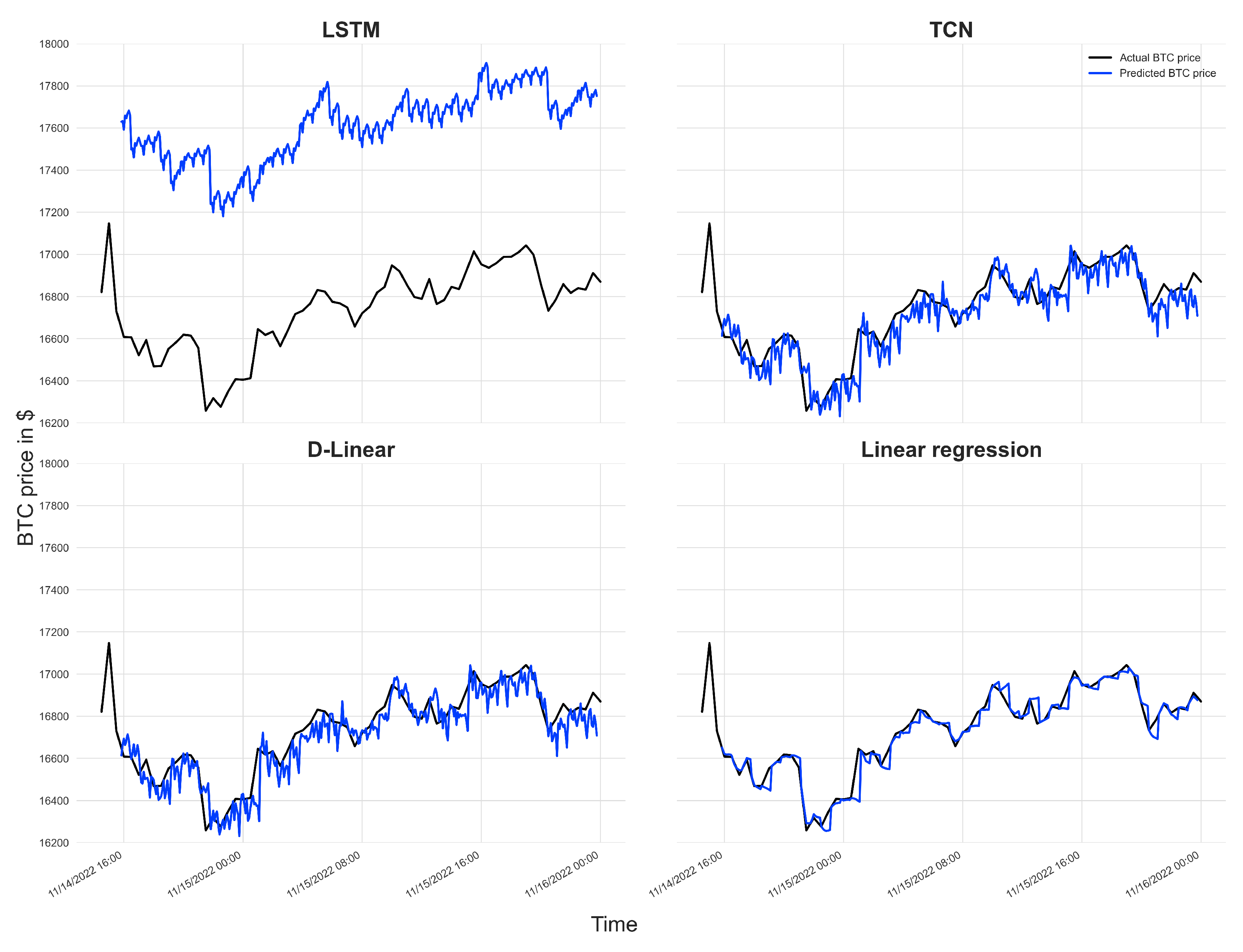
• Using this setup, we show that our approach outperforms previous ones. In particular, we empirically show that both our BERT model fine-tuned for sentiment analysis and our novel weighting scheme improve forecasts in terms of predictive accuracy (MAE and RMSE) compared to other setups. Moreover, we show that simpler models, particularly linear regression models, tend to perform best, while more complex models have issues with overfitting.

In the remainder of the article, we first give an overview of comparable approaches (Section 2). Then, we specify our methodology in detail (Section 3), first in terms of forecasting algorithms (Section 3.1) and then in terms of sentiment analysis methods (Section 3.2) and also in terms of our data setup (Section 3.3). Finally, in Section 4, we share our empirical results and discuss them both qualitatively and quantitatively. An overview of our approach is also given in Figure 1.

2. Related Work

Our work connects to two strands of research in the domain of Bitcoin price prediction: time series forecasting (Section 2.1) and sentiment analysis (Section 2.2). State-of-the-art methods combining both areas are reviewed in Section 2.3. We provide a summary table of research work related to Bitcoin price prediction with the help of sentiment scores in Table 1. We also sketch our novel contributions in this work (Section 2.4).

2.1. Time Series Forecasting for Cryptocurrencies

To obtain forecasts, there exist numerous models, ranging from very simple to highly complex [9,31]. One strand of research employs deep learning models, such as long short-term memory (LSTM) networks, to anticipate the price of BTC. These models have been successful in capturing temporal relationships in data and can be trained on vast volumes of data [31,32,33]. LSTM networks have also been successfully applied to predict the price of BTC [2,34,35,36].

Jaquart et al. [34] trained a diverse set of forecasting models to predict binary relative daily market movements of 100 cryptocurrencies, including Bitcoin, and showed that an ensemble of LSTM and gated recurrent unit (GRU) networks, both of which belong to the category of recurrent neural networks (RNNs), performs best. Uras et al. [35] utilized multi-layer perceptrons (MLPs), LSTM networks, and linear regression models to predict the price of BTC, along with the prices of other stocks, and showed that LSTM networks performed best. Patel et al. [2] and Hamayel and Owda [36] used LSTM and GRU networks to forecast the price of BTC and also that of other cryptocurrencies. Their experimental results indicate that models that perform well on BTC perform comparatively well on other cryptocurrencies, such as Ethereum, Litecoin, or Monero. Contemporary to our study, Dimitriadou and Gregoriou [37] collected 24 relevant variables, such as exchange rates or the value of other cryptocurrencies, to predict whether BTC would rise or fall. In their results, the simple logistic regression model performed the best. In another research work, three models, namely, an MLP, a support vector machine (SVM), and an LSTM network, were trained to predict the price of BTC using its historical price and several additional BTC trading indicators as input features [9]. The authors found that the SVM with comparably few trainable parameters outperforms all others, including the more complex ones. However, they failed to employ a proper, simple baseline model that does not consider any additional features other than the historical price of BTC. Moreover, Liu et al. [31] drew two conclusions that provide valuable insights relevant to our research. First, they found that, in various time series forecasting tasks, more complex models often suffer from overfitting, which they attributed to the limited availability of training data. Second, they contended that transformer networks exhibit promising results in certain time series forecasting tasks but are computationally expensive and unable to effectively capture long-term dependencies from the distant past.

2.2. Sentiment Analysis

Another strand of research aims to capture sentiment scores derived from SA techniques. In general, SA can be categorized into machine learning (ML), lexicon-based methods, and rule-based techniques [38,39]. For text found on social media platforms, one prominent method is VADER, which we describe in more detail in Section 3.2.1. VADER has been employed for a variety of tasks; for example, for tasks specific to the COVID-19 pandemic [40,41], for app recommendations [42], or for classifying complex datasets [43]. Another SA method commonly used for social media data is TextBlob [44]. In contrast to VADER SA, which derives its sentiment scores based on rules, TextBlob combines lexicon-based approaches and ML techniques [45,46]. Notably, TextBlob has also been used for emotion detection by Aslam et al. [47]. More recently, SA methods based solely on ML have gained popularity [48], for example, methods based on convolutional neural networks [49], recurrent networks [47], attention networks, [50] or transformer networks [51]. We provide more details on the latter (in particular, BERT) in Section 3.2.2.

2.3. Combining Time Series Forecasting with Sentiment Scores

In addition to the historical price of financial assets, sentiment scores have been added as an additional input feature to the model (most commonly, LSTM networks), in a number of studies, with encouraging results [52,53,54]. Furthermore, several studies have shown the ability of sentiment scores derived from the VADER SA technique to enhance the prediction of the price of BTC [10,54,55,56]. For instance, Abraham et al. [57] and Mittal et al. [58] combined sentiment scores with tweet volumes and Google Trends, respectively, to create forecasts. Moreover, Wołk [14] used ten different forecasting models to predict the price of several cryptocurrencies, including Bitcoin, and showed that psychological and behavioral aspects have a strong impact on prices. In a recent study, Ye et al. [54] created a stacking ensemble consisting of LSTM and GRU networks to predict the price of BTC based on historical price data, various technical indicators, and VADER-derived sentiment scores. Their results indicate that the combination of multiple model outputs through stacking can improve forecast accuracy and that both technical indicators and sentiment scores improve forecast accuracy. Likewise, Serafini et al. [13] employed two distinct models in their research, namely, an ARIMAX model and an LSTM model, to forecast BTC prices. The authors conducted experiments using various combinations of sentiment and financial input features. In particular, their findings revealed that the inclusion of additional input features, such as the BTC trading volume or the tweet volume, did not necessarily improve the forecasting capabilities. This observation, which may seem counterintuitive for this specific task, served as a key motivation for our study. Our aim is to investigate the analysis of optimal combinations of characteristics and explore possible adjustments to improve the performance of forecasting models.

Furthermore, they found that although the ARIMAX model they employed is simpler it outperformed the more complex LSTM model. In another study, Edgari et al. [59] used XGBoost, an implementation of a gradient-boosted decision tree, to estimate the price of BTC during the COVID-19 pandemic. They used a dataset comprising tweets that date from February 2021 to December 2021 and aggregated tweets into 1-min time windows. To obtain sentiment scores, they applied VADER SA and used the average of the compound score as the sentiment score for a given 1-min time interval. In addition to sentiment scores, they added the average of user-related features over all users who created a tweet in a given 1-min interval as input to the model, such as the number of followers, favorites, and whether the user is verified or not. Finally, they predicted whether the price associated with the next time step rises or falls, thus creating a binary classification task. Using the aforementioned XGBoost model to make predictions, the authors concluded that sentiment scores are indeed helpful for forecasting BTC prices. A summary table of the research works related to the prediction of BTC prices with the help of sentiment analysis techniques is shown in Table 1.

Table 1. Summary of related work on BTC price prediction leveraging sentiment scores. Year corresponds to the publication year. Pred. target refers to the forecasting target of the BTC price: binary means that the objective is to predict whether BTC will increase or decrease, and value means that the objective is a direct prediction of the BTC price. Granularity corresponds to the degree to which the data are aggregated for prediction. Model corresponds to the set of forecasting models used. Additional features lists the features that are added in addition to the historical BTC price.

Ref.	Year	Pred. Target	Granularity	Model	Additional Features
[55]	2020	binary	1 min	random forest	VADER SA
[54]	2022	value	30 min	stacking ensemble of LSTM, GRU	VADER SA, trading features
[56]	2022	value	12 h	vector autoregression	VADER SA
[57]	2018	value	1 day	linear regression	VADER SA, tweet volume, Google Trends
[58]	2019	value	1 day	LSTM, vanilla RNN, linear regression, polynomial regression	VADER SA, tweet volume, Google Trends
[14]	2019	value	1 day	10 different models	VADER SA, Google Trends
[13]	2020	value	1 day	LSTM, ARIMAX	VADER SA, tweet volume
[59]	2022	binary	1 min	XGBoost	VADER SA, tweet volume, user-related features

Table 1. Summary of related work on BTC price prediction leveraging sentiment scores. Year corresponds to the publication year. Pred. target refers to the forecasting target of the BTC price: binary means that the objective is to predict whether BTC will increase or decrease, and value means that the objective is a direct prediction of the BTC price. Granularity corresponds to the degree to which the data are aggregated for prediction. Model corresponds to the set of forecasting models used. Additional features lists the features that are added in addition to the historical BTC price.

Ref.	Year	Pred. Target	Granularity	Model	Additional Features
[55]	2020	binary	1 min	random forest	VADER SA
[54]	2022	value	30 min	stacking ensemble of LSTM, GRU	VADER SA, trading features
[56]	2022	value	12 h	vector autoregression	VADER SA
[57]	2018	value	1 day	linear regression	VADER SA, tweet volume, Google Trends
[58]	2019	value	1 day	LSTM, vanilla RNN, linear regression, polynomial regression	VADER SA, tweet volume, Google Trends
[14]	2019	value	1 day	10 different models	VADER SA, Google Trends
[13]	2020	value	1 day	LSTM, ARIMAX	VADER SA, tweet volume
[59]	2022	binary	1 min	XGBoost	VADER SA, tweet volume, user-related features

2.4. Research Gaps and Novel Contributions

Reviewing related work, we identified research gaps concerning (1) the period spanned by the investigated datasets and the corresponding BTC price ranges, (2) the use of more up-to-date and sophisticated SA and ED techniques, and (3) the use of appropriate baselines. Furthermore, we have not encountered studies that predict not only one but multiple time steps into the future. Addressing these gaps, what sets the article at hand apart from previous research is that we use a dataset spanning a longer period and more diverse price ranges. Moreover, we employ not only VADER SA but also BERTweet-based SA and ED. Additionally, we utilize a distinct set of forecasting models, including appropriate baselines. The dataset we use comprises tweets from February 2021 up to November 2022, which makes it more recent and covers a longer period as well as more diverse price ranges compared to the one used by Edgari et al. [59] and other previous studies. Furthermore, we conduct our investigation over a 30-min period rather than a 1-min period, as employed by Edgari et al. [59]. This enables us to gain a more complete understanding of the market sentiment and its influence on the price of BTC over time. Moreover, instead of the more conventional way of predicting the price of a given asset in a time step $p_{T+1}$ using the prices of $p_T,p_{T-1},...,p_{T-N}$, where N may vary, we predict M time steps, with $M>1$, thus predicting the price of BTC for multiple time steps into the future. Although more challenging, this approach allows for a longer forecast period, ranging from $p_{T+1}$ to $p_{T+M}$. Consequently, it integrates the performance assessment of short- and mid-term forecasts using just a single unified model. Predicting multiple time steps into the future enhances the forecasting horizon, offering flexibility and adaptability in decision making to align with different potential future scenarios. It also allows for the assessment of the model’s performance across different time frames, contributing to a more holistic understanding of market dynamics and providing insights into the model’s stability over time. Moreover, to the best of our knowledge, we are the first to use BERT-based sentiment analysis techniques to enrich the historical price of BTC with sentiment scores, along with emotion detection scores, combining these unique forecasting characteristics.

3. Methodology

In the following, we provide a brief overview of the overall task as well as our approach. The exact methodology of our hybrid BTC price forecasting algorithm will be explained in more detail in the upcoming sections.

As visually described in Figure 2, we first gather data on both the historical price of BTC and the time-aligned tweets, from which sentiments are extracted. The textual tweet dataset is then pre-processed using standard NLP techniques, cleaned, and subjected to three distinct types of SA methods. Next, we generate sentiment scores for each tweet. For that, we use two distinct approaches, namely, VADER, which relies on rules, and different variations of a BERT model, which is an ML model that can capture the relations between words more richly compared to traditional rule-based methods. We group the output into bins of 30-min intervals based on the corresponding tweets’ time stamps and then use two distinct methods to weigh the derived sentiment values. The last step of data pre-processing is to prepare the data so that it can be used as input to various forecasting methods.

Finally, as can be visually observed in Figure 1, we feed the prepared data into our ML models. We use 16 30-min intervals, that is, 8 h, as input and predict 8 30-min intervals, that is, 4 h, for all our forecasts. To predict the future price of BTC, we employ four different types of models: linear regression (LR), LSTM networks [60], temporal convolutional networks (TCNs) [61], and the D-Linear method [62], each of which uses a unique set of covariates.

In the next sections, we outline the forecasting algorithms used (Section 3.1), specify our method to compute sentiment scores (Section 3.2), and outline the data acquisition procedure, as well as the processing steps (Section 3.3).

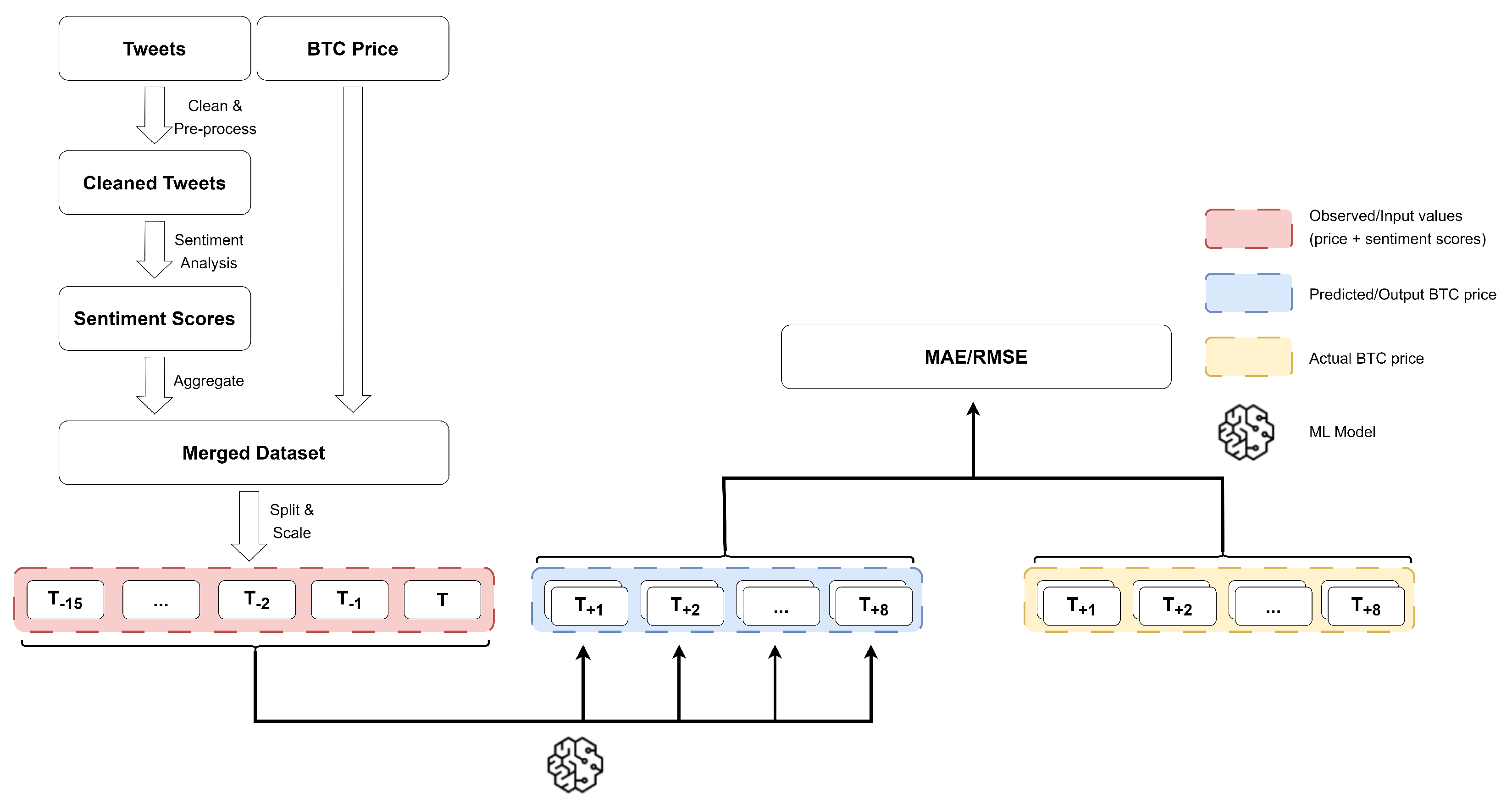
3.1. Forecasting BTC Price

We conduct most of our forecasting experiments with the Darts [63] framework, which is based on PyTorch [64]. We feed 16 30-min intervals, i.e., 8 h, as input to our models and predict 8 30-min intervals, i.e., 4 h, for all our forecasts. These values are chosen to reflect the characteristics of intraday trading. We evaluate the final performance on the test set, which has not been considered at all until the final evaluation. We use the validation set to select the best hyperparameter setup for each model, including early stopping. More information on how we split the data is given in Section 3.3.

Forecasting Algorithms. In our hybrid BTC price forecasting algorithm, we investigate four types of ML-based algorithms: LSTM networks, TCNs, the D-Linear method, and linear regression, along with some simple baselines. We decide to use LSTM networks and TCNs since both have shown remarkable success in a variety of forecasting tasks [14,34,53,65,66], making them a very common choice for models with high complexity. Moreover, we decide to use the D-Linear method and linear regression since both have shown potential in making accurate forecasts while being comparatively simple [35,62,67,68]. For forecasting, all our baselines rely solely on the price and do not require any training. The other models that are employed, except for the LR model, are all trained with the following commonalities: We train each of them for 50 epochs using the mean squared error (MSE) loss function and the Adam optimizer, but we use early stopping if the loss on the validation set does not decrease for five consecutive epochs. Additionally, if the training loss does not decrease for three successive epochs, we cut the training rate by half. More details on hyperparameter selection are provided in the following subsections that detail the algorithms used.

3.1.1. Baselines

Exponential Smoothing. Exponential Smoothing (ES) is a time series forecasting method that uses a weighted average of past observations to predict future observations [69]. The weights decrease exponentially as observations come from further in the past; the smallest weights are associated with the oldest observations. It is a generalization of the simple moving average, where all weights are equal. We use Holt–Winters’ ES [70] with additive seasonality as well as trends and consider two periods in each seasonal cycle.

Fast Fourier Transform. The Fast Fourier Transform (FFT) decomposes the time series into its frequency components [71,72], which are then used to predict future values of the time series. It is particularly suitable for highly seasonal data. We use the standard Darts hyperparameters.

Naive Mean. The Naive Mean model simply predicts the mean value of the input series. Hence, in our case, it predicts the mean value of the last 16 BTC price values.

Naive Drift. The Naive Drift Model extends the line between the first and last point of the training series into the future [63].

3.1.2. Long Short-Term Memory Network

The long short-term memory (LSTM) network, as introduced by Hochreiter and Schmidhuber [60], is a type of recurrent neural network used for sequence prediction problems. The network has memory, which allows it to learn from sequences of input data. The LSTM model consists of memory blocks that are linked together. Each block has a memory cell that is connected to gates that control the flow of information into and out of the memory cell. The LSTM model is trained by unrolling the network and presenting the input sequence one element at a time to the network. LSTM networks have been used successfully for a variety of tasks, including time series forecasting [32,33]. To predict multiple time steps into the future, the LSTM network learns a single-step forecast and iteratively applies it to obtain multi-step forecasts (in our case, 8). Hence, it can be characterized as autoregressive.

We train LSTM networks with a batch size of 2048, a learning rate of 0.0003, and a dropout rate of 0.1. Moreover, we use LSTM networks with two layers with a hidden dimension of size 512 and append two fully connected layers with sizes $[512,128]$ to the hidden layers.

3.1.3. Temporal Convolutional Networks

Temporal convolutional networks (TCNs) are a class of neural networks that are designed to operate over sequences of data, such as time series [61,73]. TCNs consist of a stack of convolutional layers, pooling layers, and fully connected layers. The convolutional layers are comprised of filters (kernels) that are applied to the input sequence; pooling layers are used to down-sample the output of the convolutional layers; and the fully connected layers are used to interpret the features extracted by the convolutional and pooling layers.

We train TCNs with a batch size of 512, a learning rate of 0.001, and a dropout rate of 0.2. We use TCNs with 16 kernels of 8, 12 layers, and 2 as a dilation base. Moreover, we apply weight normalization to stabilize the training process.

3.1.4. D-Linear

The D-Linear model is a novel time series forecasting method based on a single-layer neural network [62]. First, it decomposes the input data into a trend by applying a moving kernel average and a remainder (seasonal) component. Second, two single-layer linear layers are applied to each component. Ultimately, the two features are summed up to obtain the final predictions. Therefore, it has comparatively few parameters.

We train the model with a batch size of 2048, a learning rate of 0.01, and no dropout. Moreover, we use a kernel size of 25 for the moving kernel average computation.

3.1.5. Linear Regression

Linear regression is a statistical method for modeling the relationship between a dependent variable y and one or more explanatory variables (or independent variables) denoted by X [74]. Since we rely on more than one explanatory variable, we conduct multiple LR models. We perform least squares regression to find the best-fitting line for the data, which is the line that minimizes the MSE between the predicted and target values. To generate predictions for multiple time steps, we train a separate model for each future time step. This results in eight independent models for our approach, each corresponding to a single future time step.

3.2. Sentiment Analysis

The purpose of sentiment analysis, a branch of natural language processing, is to discover the general view or attitude of a speaker or writer toward a certain topic or issue automatically [38,39]. Machine learning, lexicon-based methods, and rule-based approaches are some of the techniques that may be utilized for SA [38,39].

In our study, we rely on two distinct SA approaches: The first is VADER, which relies on a set of rules and has been used successfully in many studies [10,55,56,59]; but it cannot capture the relations between words. It is specifically designed for social media data. The second relies on BERT, which has shown great promise in various NLP tasks, including SA and ED. Since BERT is a general-purpose model, we use fine-tuned variants of BERT that suit our hybrid BTC price forecasting algorithm.

3.2.1. VADER Sentiment Analysis

VADER is an SA method that has been specifically designed for social media data [26]. The rule-based model has become one of the most popular since its introduction in 2014 [10,11,59,75]. To define these rules, the authors introduce a combination of qualitative and quantitative methods to generate a “gold-standard” lexicon that is specially tuned for social media text, all while following an “explicit human-centric approach”. Hence, each word in the English language is associated with a sentiment polarity (positive/negative) and sentiment intensity. These scores are aggregated to obtain scores for a single passage or document. Finally, upon qualitative analysis, the authors decide to use further heuristics incorporating word-order sensitive relationships between terms, namely, punctuation, capitalization, degree modifiers, “but” as a sentiment polarity shifter, and catching negation flips by considering tri-grams. These heuristics modify the score of a given passage or document. For each piece of text, VADER outputs four kinds of sentiment scores: positive, negative, and neutral, corresponding to sentiment polarity with a given intensity, and a compound score. For the SA methods, we conduct experiments using all scores but also only using the compound score as input to the model in addition to the historical price data.

To obtain sentiment scores using VADER, we use the open-source Python implementation provided by the authors of the original paper [76].

3.2.2. BERT-Based Sentiment Analysis

BERT is a pre-trained transformer model that has been successfully applied to a wide variety of tasks and domains [29]. The attention mechanism employed in these models allows them to capture the context, specifically the surrounding words in the sentence. We rely on two different, fine-tuned versions of BERT, each of which outputs a distinct set of sentiment features. Both rely on BERTweet [30], which is a version of BERT that has been further trained on English tweets.

Despite being much more computationally expensive than VADER, we employ BERTweet-based SA and ED models, since both models have shown state-of-the-art performance on their respective tasks [30]. Moreover, they have not yet been used to predict the price of BTC to the best of our knowledge.

To obtain sentiment scores using BERTweet-based SA and ED models, we use the respective models for English, as provided by the open-source Python library pysentimiento [51].

BERTweet-based sentiment analysis. The first specialized model is a BERTweet-based SA model for English tweets. It starts from the weights of BERTweet and further fine-tunes them on the SemEval-2016 dataset [77], which is an SA dataset. For each piece of text, it produces three types of sentiment scores: positive, negative, and neutral. In addition, we define a compound score, which simply consists of subtracting the negative score from the positive score.

BERTweet-based emotion detection. The second specialized model is a BERTweet-based ED model for English tweets. Again, it starts from the weights of BERTweet, but this time it is further fine-tuned on the EmoEvent dataset [78], which is an ED dataset. For each piece of text, it produces seven scores, each corresponding to a distinct emotion: joy, sadness, anger, surprise, disgust, fear, and, additionally, a score for others. We have decided to also include ED since emotions enable a more nuanced distinction of sentiment towards BTC compared to only using positive, negative, and neutral scores, which also improves interpretability. In this setup, we use all seven emotion scores as input to the model, in addition to the historical price data.

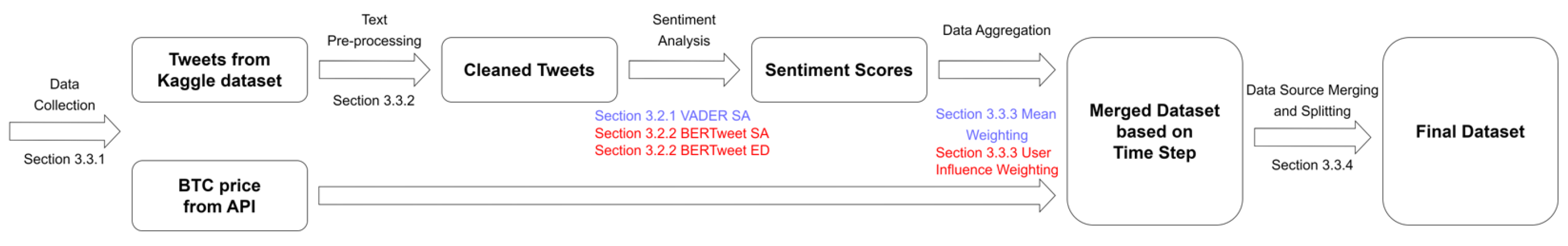
3.3. Data Acquisition and Processing

In the following, we outline our data acquisition and processing approach. First, we describe how we collect our data (Section 3.3.1) and how we pre-process the tweets (Section 3.3.2). Then, we explain how we aggregate multiple sentiment scores of tweets from a given time interval into a single sentiment score for the given time interval (Section 3.3.3). Finally, we show how we merge our two data sources and how we split the data into train, validation, and test sets (Section 3.3.4). Our data and pre-processing pipeline is shown in Figure 2.

Figure 2. Overview of our data acquisition and pre-processing pipeline. After having collected both BTC prices and relevant tweets, we pre-process the text, resulting in cleaned tweets. Next, we derive sentiment scores using VADER SA, BERTweet SA, and BERTweet ED. Based on these sentiment scores, we aggregate multiple tweets using two different weighting schemes. Finally, we merge the two datasets and split the data into train, validation, and test sets. Previous methods are marked in blue, whereas our introduced methods are in red.

Figure 2. Overview of our data acquisition and pre-processing pipeline. After having collected both BTC prices and relevant tweets, we pre-process the text, resulting in cleaned tweets. Next, we derive sentiment scores using VADER SA, BERTweet SA, and BERTweet ED. Based on these sentiment scores, we aggregate multiple tweets using two different weighting schemes. Finally, we merge the two datasets and split the data into train, validation, and test sets. Previous methods are marked in blue, whereas our introduced methods are in red.

3.3.1. Data Collection

For our evaluation experiments, we require some historical BTC price data as well as tweets. We leverage the Binance API [79], which offers price data at 30-min intervals, to obtain the information for the BTC price. We use the BTC-USDT pair, as USDT (Tether) is the stablecoin with one of the highest market caps tied to the US Dollar, which in turn is the most significant currency for worldwide trading. Hence, this provides a realistic scenario from the point of view of a trader.

Secondly, to obtain sentiment scores that are calculated based on tweets from Twitter, we use a dataset from Kaggle [80], which consists of tweets with the hashtag #BTC or #Bitcoin. Furthermore, the dataset consists of tweets spanning from 10 February 2021 to 20 November 2022. This period saw particularly volatile BTC prices. Later, forecasting these prices from these diverse ranges proved to be a significant challenge. The dataset consists of 4.5 million relevant tweets in total, with 11 attributes each. For our use case, only the attributes “text” (i.e., the content of the tweet), “date” (the exact time of creation), and “user_followers” (i.e., how many followers the author of the tweet had at the time of posting) are of relevance. However, the dataset comes with one limitation: there are numerous temporal gaps—periods when there were no tweets at all. They frequently lasted for several weeks and, in fact, more than half of the days lack any tweet data. Therefore, we had to discard these time periods, which also significantly reduced the amount of data on which we could reliably train our models. However, we still opt to use this dataset, as it is quite large. Moreover, one major goal of this study was to see how well models generalize over unseen price ranges and market conditions; for that, we needed a dataset that spans periods corresponding to varying market conditions. This also clearly differentiates our setup from those used in previous studies and makes it more useful for real-life use cases.

3.3.2. Text Pre-Processing

The dataset is first cleaned using common practices as employed in the literature as part of our text pre-processing process [12,56,59]. We eliminate non-English tweets with langdetect [81] and tweets with fewer than three characters. We also replace over two (or more) subsequent dots with a space, remove multiple spaces, and remove words with only one character with the Python-based open-source library Pandas. After having cleaned the dataset, 458,472 tweets remain for further pre-processing. Subsequently, we prepare the text in a format with which our sentiment analysis methods work well. This process is different for our different approaches. To prepare the data for VADER, we lowercase the tweets; remove @, $, and # signs; and remove stopwords. Although both methods have been used in the related literature [12,56], we choose not to lemmatize or stem the text because in our dataset there are many domain-related terms, abbreviations, and jargon that may not necessarily benefit from common lemmatization or stemming techniques. To prepare the data for BERT-based SA, we follow the process described by Pérez et al. [51]: # signs, @ signs, and URLs are replaced with special tokens (and not removed, as performed for VADER), and emojis are converted to their text representations.

3.3.3. Data Aggregation

Having sentiment scores for each tweet, the next step is to aggregate the sentiment of all tweets from a given 30-min interval into a single sentiment score corresponding to the overall sentiment in a given time period (in our case, 30-min). There exist different ways to weigh the scores, such as taking the mean, median, or sum of all the sentiment scores. We conduct experiments with two different weighting schemes. For each of them, we independently weigh the different scores of each SA method.

Mean weighting. The first is to simply take the mean sentiment score of all tweets in each 30-min interval. In other words, we compute

$$\sum _{i=1}^n\frac{s\left(x_i\right)}{n},$$

where $s\left(x_i\right)$ is the sentiment score of a tweet $x_i$ in the current 30-min interval, and n is the number of tweets in this interval.

Weighting by number of followers. The second one, which we will refer to as user influence weighting, relies on the assumption that Twitter users with more followers are more influential and therefore presumably more relevant. Based on this, we arrive at the following novel weighting scheme:

$$\frac{{\sum }_{i=1}^{n}s\left(x_i\right)\left(ln(w_i+1)+1\right)}{{\sum }_{i=1}^{n}ln(w_i+1)+1},$$

where $s\left(x_i\right)$ is the sentiment score of a tweet $x_i$ in the current 30-min interval, and $w_i$ is the number of followers the author of the tweet had at the time of creation. We use the logarithm to dampen the effect of users with a very large number of followers, inspired by the retrieval method BM25 [82].

3.3.4. Data Source Merging and Splitting

Finally, we merge the two data sources, namely, historical BTC prices and sentiment scores from Twitter, into a single data source, which can be neatly achieved by matching their respective time steps. Next, we split the data into train, validation, and test splits based on time to counteract the “peek-a-boo” anti-pattern [83], which would be violated if we used a random or stratified split based on the target value, an otherwise common practice in ML. We used 80% of the available data for training and 10% as validation and test sets, respectively. Using this splitting strategy, the training data spans from 11 February 2021 up to 6 June 2022; the validation data from 14 June 2022 up to 6 September 2022; and the test data from 11 September 2022 up to 20 November 2022. The gaps in the respective sets are due to the gaps in the dataset because we want to avoid splitting during a period with a gap. Note that the size of the splits does not depend on the date but rather on the number of 30-min intervals available during a given time interval. Finally, we standardize the data based on the values in the training set.

We also experimented with additional feature engineering, including exponential moving averages, temporal features such as the day of the week or holidays, and the total number of tweets in each time interval (i.e., tweet volume). However, none of these significantly improved performance metrics in our experiments. We assume that this may be due to the highly volatile nature of BTC.

4. Evaluation and Discussion

In this section, we present the results of our main experiments, which aim to evaluate the performance of the investigated BTC price forecasting algorithms. First, we provide a comprehensive overview of the performance of all algorithms, including baselines, when only considering the price as input. Next, we compare the performance of all of the algorithms that we used with varying input features, using the mean weighting scheme. This gives us a better understanding of how each algorithm performs with different sentiment scores. Afterward, we compare the performance of the mean weighting scheme with our user influence weighting scheme. We demonstrate how our user-influenced weighting scheme affects the overall performance of the algorithms and identify if it outperforms the mean weighting scheme. Overall, these experiments provide us with a better understanding of how each algorithm performs under various conditions and help us determine the most efficient algorithm and weighting scheme for our study. By analyzing the results of these experiments, we are able to identify the most suitable algorithm and combination of features to predict the price of BTC.

For reference, the minimum price of BTC during the entire period was USD 15,704, while the maximum value was USD 68,633, with the latter occurring during the training set period. However, the minimum price of the training set was USD 27,114, whereas the minimum price occurring during the test set period was USD 15,704. The maximum price that occurred during the period of the test set was USD 22,713. This divergence highlights the difference between the training and test set price ranges. Therefore, in order to perform well on the test set, our models need to have good generalization capabilities.

We evaluate all our models on the test set using the RMSE (root mean squared error) and MAE (mean absolute error) error metrics. Since we compute multiple forecasts, we consider every output prediction, compare it with the ground truth, compute the respective error metric over our eight forecasting time steps, and then take the average, as can be seen in Figure 1. Then, we move one time step forward and again compute the same metric over the next eight forecasting time steps. The final results, as reported in

Table 2. Comparison of performance of forecasting algorithms on the test set using only the BTC price as input, with data spanning from 5 February 2021 up to 20 November 2022. The best score for a given feature combination is marked in bold, and the second best is underlined. Columns on the right indicate the different forecasting algorithms, as specified in Section 3.1. All of them use the BTC price as the only input attribute. We conduct a permutation test to determine statistical significance between our best models and the other models. † indicates that all of the LR, D-Linear, ES, and Drift models perform significantly better ($p<0.05$) than all other models with worse performance.

Metric	LSTM	TCN	D-Linear	LR	ES	FFT	Drift	Mean
MAE	11.69	13.71	3.40  ${}^{†}$	2.72  ${}^{†}$	4.15 ${}^{†}$	9.46	3.43 ${}^{†}$	7.13
RMSE	12.22	14.19	4.22 ${}^{†}$	3.33  ${}^{†}$	5.01 ${}^{†}$	10.04	3.97  ${}^{†}$	7.51

,

Table 3. Comparison of performance of algorithms and SA techniques on the test set using mean weighting, with data spanning from 5 February 2021 up to 20 November 2022. The best score for a given feature combination is marked in bold, and the second best is underlined. Columns on the right indicate the different forecasting algorithms, as specified in Section 3.1. Rows indicate the covariates used as inputs to the different forecasting algorithms, depending on the SA method employed. All scores means that all the sentiment scores are used as covariates, while compound score corresponds to only using the compound score that is calculated based on the other scores as a covariate. All setups use the past price of BTC, as described in Section 3, as input. We conduct a permutation test to determine statistical significance between our best models and the other models. † indicates that both the LR and D-Linear models perform significantly better than the other models, while ‡ indicates that our LR model is better than all other models with worse performance, including D-Linear. Both † and ‡ correspond to $p<0.05$.

SA Method	Scores	Metric	LSTM	TCN	D-Linear	LR
VADER SA	All	MAE	90.50	19.22	4.49  ${}^{†}$	3.23  ${}^{†}$
		RMSE	90.67	19.69	5.48  ${}^{†}$	3.96  ${}^{†}$
	Compound	MAE	25.81	12.84	3.46  ${}^{†}$	2.71  ${}^{†}$
		RMSE	26.17	13.37	4.23  ${}^{†}$	3.31  ${}^{†}$
BERTweet SA	All	MAE	53.32	22.72	4.75  ${}^{†}$	3.14  ${}^{†}$
		RMSE	53.09	22.18	5.93  ${}^{†}$	3.85  ${}^{†}$
	Compound	MAE	35.04	11.56	3.75  ${}^{†}$	2.67  ${}^{†}$
		RMSE	35.41	12.10	4.75  ${}^{†}$	3.28  ${}^{†}$
BERTweet ED	All	MAE	22.39	15.49	6.35	2.87  ${}^{‡}$
		RMSE	22.94	16.07	8.02	3.52  ${}^{‡}$

and

Table 4. Comparison of performance of algorithms and different weighting schemes on the test set using all sentiment scores, with data spanning from 5 February 2021 up to 20 November 2022. The best score for a given feature combination is marked in bold, and the second best is underlined. Columns on the right indicate the different forecasting algorithms, as specified in Section 3.1. Rows indicate the covariates used as inputs to the different forecasting algorithms, depending on the SA method employed. Mean weighting and user influence weighting refer to the different weighting schemes introduced in Section 3.3.3. We conduct a permutation test to determine statistical significance between our best models and the other models. † indicates that both the LR and D-Linear models perform significantly better than the other models, while ‡ indicates that our LR model is better than all other models with worse performance, including D-Linear. Both † and ‡ correspond to $p<0.05$.

SA Method	Weighting	Metric	LSTM	TCN	D-Linear	LR
Vader SA	Mean	MAE	90.50	19.22	4.49  ${}^{†}$	3.23  ${}^{†}$
		RMSE	90.67	19.69	5.48  ${}^{†}$	3.96  ${}^{†}$
	User influence	MAE	132.54	25.55	4.37  ${}^{†}$	3.35  ${}^{†}$
		RMSE	132.66	25.98	5.36  ${}^{†}$	4.11  ${}^{†}$
BERTweet SA	Mean	MAE	53.32	22.72	4.75  ${}^{†}$	3.14  ${}^{†}$
		RMSE	53.09	22.18	5.93  ${}^{†}$	3.85  ${}^{†}$
	User influence	MAE	53.09	10.13	4.53  ${}^{†}$	3.01  ${}^{†}$
		RMSE	53.33	10.78	5.68  ${}^{†}$	3.69  ${}^{†}$
BERTweet ED	Mean	MAE	22.39	15.49	6.35	2.87  ${}^{‡}$
		RMSE	22.94	16.07	8.02	3.52  ${}^{‡}$
	User influence	MAE	36.13	14.43	5.97	2.84  ${}^{‡}$
		RMSE	36.48	14.95	7.36	3.49  ${}^{‡}$

, are obtained by computing the arithmetic mean of the averages of the computed error metrics.

To investigate whether our best models are significantly better than the other models, we make use of statistical testing. To accomplish this, we first test whether our dataset is stationary or normally distributed, since some commonly used tests, such as ANOVA, require normally distributed samples. To check whether the data are normally distributed, we use the Shapiro–Wilk test. The test reveals that the dataset does not follow a normal distribution. We also employ a quantile–quantile (qq) plot to visually check the data to verify our findings. Moreover, to check stationarity, an important aspect, we conduct a Kwiatkowski–Phillips–Schmidt–Shin (KPSS) test. On the basis of this test, we conclude that Bitcoin price data are non-stationary, which might be associated with their highly volatile nature in general. Moreover, we use the statsmodels Python library to split the price data into seasonal, trend, and residual components. Based on these components, we find that the time series does not display a significant seasonal pattern. Moreover, we notice a declining tendency in the validation set but not in the training set. Finally, we validate the time series by plotting the autocorrelation function (ACF) and partial autocorrelation function (PACF) of the BTC price. In summary, the results of the ACF plot (e.g., 0.5 at lag 20) indicate a moderate correlation between the current value and its past values up to lag 20. However, the PACF plot indicates a very strong correlation of almost 1 of the first 2 lags with the current value, while lags from the third and onward show a correlation closer to 0, suggesting that the current value becomes less dependent on its past values beyond the immediate two lags. By conducting these tests and analyzing the results, we gained valuable insights into the properties of the Bitcoin datasets, which will inform our subsequent modeling and analysis. Furthermore, it helps in choosing the appropriate statistical test. Based on our findings, using the results on the test set of all models, we conduct a permutation test, as it is more robust w.r.t. different sample distributions and, hence, more robust than the commonly used t-test. Using this test, we use a high permutation number of 1,000,000 to obtain a higher precision of the p-value, resulting in a standard deviation of only 1.2 × 10⁻⁴. In the following, we discuss a few observations, both in terms of models and features.

4.1. Model Comparison

First, we compare our different models with each other: LR, D-Linear, TCN, and LSTM. The results are shown in Table 3.

Models with a lot of parameters (LSTM and TCN) are prone to overfitting, which is a typical problem that occurs when a model is overly sophisticated and can recall the training data but fails to generalize to new data, i.e., test data. Indeed, they perform very well on the training set but perform poorly on the test set. Specifically, the variance in their predictions on the test set is very high, and their predictions are generally too high. Increasing regularization, such as dropout or weight decay, did not ameliorate their weak performance. We hypothesize that this may be due to not using enough training data and that the gaps in the training set in particular hurt their generalization performance significantly. Second, the D-Linear model performs decently but not as well as LR. Compared to the baselines, it is only better in terms of the MAE. As an ultimate observation, we see that LR is by far our best model. It does not have issues with overfitting and is also the fastest to train. We hypothesize that this may be due to the unconventional method we have chosen, i.e., fitting a single LR model for each output prediction.

Figure 3 shows the performance of our models on the last segment of the test set using mean weighting and all sentiment scores. The results indicate that the more complex models in particular have difficulties with previously unseen price ranges and market conditions observed in the test set periods. The predictions of the complex LSTM and TCN models are rather unstable and always overestimate the true price, indicating that they are unable to generalize. In contrast, the simpler D-Linear model predicts the correct price ranges more accurately but is still unstable. Finally, the LR model predicts the general price ranges well while also making the best forecasts, showing its superior generalization capabilities.

4.2. Feature Comparison

Next, we compare our different feature setups with each other using only the price, using the price and VADER, using the price and BERTWeet SA (all sentiment scores vs. only the compound score), and using the price and BERTWeet ED using all scores. The results are shown in Table 3.

First, the combination of the BERTweet SA compound score and an LR model yields the highest overall performance. However, BERTweet SA with the compound score alone is not always the best combination of features. Second, for both VADER and BERTweet SA, leveraging the compound score only instead of all the features performed generally better. This seems surprising, especially for the more sophisticated models, which should have the capability to capture what is meaningful and what is not. However, this possibility may have been impeded by the temporal gaps in our data. In addition, BERTweet SA works slightly better than VADER SA. This is exemplified by our best model, which relies solely on the BERTweet SA compound score. However, which one is better depends heavily on the specific model and feature combination. Another observation we make is that BERTweet ED works decently. In most cases, it works better than providing all SA scores (for both VADER and BERTweet) but worse than providing only the compound scores. In general, we find that sentiment scores provide assistance only in specific situations, as is evident from a comparison between Table 2 and Table 3. For the more complex models, it even hurts their average performance. We suspect that this may be due to not having enough training data to generalize to these unseen domains and, especially, price ranges.

4.3. Weighting Comparison

Next, we compare the mean weighting scheme (as used above) with our user influence weighting scheme (see Section 3.3.3). The results are shown in Table 4.

Again, we want to highlight a couple of observations. First, except for VADER SA, our novel user influence weighting scheme aids in every feature/model combination (except for LSTM + BERTweet ED, which is an outlier). Sometimes it increases predictive performance by a large margin (e.g., greater than 2× improvement for TCN + BERTWeet SA). This underlines the merits of our method. However, for VADER SA, our user influence weighing scheme slightly decreases the predictive performance for all but one model (D-Linear), but only insignificantly. Therefore, we conclude that our method encourages further experiments using our user influence weighting, and, additionally, the exploration of other weighting schemes.

4.4. Comparison with Other Research Works

Additionally, we compare our hybrid BTC price forecasting algorithm with other, similar research works in terms of experimental setup and design. However, comparing our research work directly with others is not possible since we employ a unique forecasting scheme and dataset.

To predict the next 4 h price of BTC, we use a combination of sentiment scores derived from microblogs and historical BTC price data from the previous 8 h for each prediction. Serafini et al. [13] utilized an ARIMAX and an LSTM model to predict the price of BTC of the next day, while Edgari et al. [59] utilized an XGBoost model to classify whether BTC would rise or fall in the next minute. Hence, both comprise highly different periods. Both research works employ a similar approach by first collecting historical BTC price data and tweets for SA, be it by simply using it from Kaggle [59] or by using a web scraper [13]. Both used VADER to derive sentiment scores for a single tweet. Edgari et al. [59] used accuracy, the AUC (area under curve), and the F1-score as error metrics and showed that adding sentiment scores as inputs to the model considerably improved the performance with respect to each metric. With added sentiment scores, they were able to predict whether BTC would rise or fall with an accuracy of 90%. Serafini et al. [13] showed that the ARIMAX model outperforms the more complex LSTM model, and, using the ARIMAX model, achieved an MSE of 0.14%. Interestingly, they found that using a lower number of features produces better forecasts compared to using more features, which coincides with our findings.

However, it must be noted that the datasets used by both methods comprise totally different time periods and price ranges compared to ours—specifically, Serafini et al. [13] used data from April 2017 to October 2019, while Edgari et al. [59] used data from February 2021 to December 2021. Although our hybrid method shows higher error metrics compared to the work of Serafini et al. [13], our evaluation is both more robust and realistic, since it spans more diverse price ranges and market scenarios. Moreover, we use more models for comparison, employ two other SA techniques based on BERTweet, and improve the forecasts with our novel weighting scheme. The period under consideration in the work of Edgari et al. [59] is even shorter and, hence, makes evaluating their method very limiting and only useful for the employed 1-min period. In addition, we also employ proper baselines, which both research works we compare with lack [13,59]. Since our work does not feature any of the limitations mentioned, we argue that it is more useful compared to previously employed research works. Other approaches, as specified in Section 2, are even more dissimilar to ours, making any comparison unfeasible.

5. Conclusions and Future Work

In this article, we propose a new hybrid method for predicting the price of Bitcoin, using historic prices and affective cues from tweets. Our method integrates time series forecasting techniques with SA and ED based on a BERTweet model. It also adopts a novel weighting scheme to aggregate multiple sentiment scores from a given time period into a single sentiment score, factoring in the importance or influence of Twitter users. We investigate our method on a dataset spanning long and diverse price ranges and show that our approach outperforms previous methods in terms of predictive accuracy. Our empirical results indicate that sentiment scores derived from both VADER and BERTweet can help investors make better forecasts, which supports the hypothesis set in Section 1. Based on our findings, we suggest using simple models such as linear regression to predict the price of Bitcoin instead of more complex ones, particularly if the amount of available data is limited. Moreover, we suggest using BERT-based SA techniques and experimenting with weighing the influence of sentiment scores.

Forecasting the price of BTC is a very challenging task because it is a highly volatile asset. To acknowledge this fact, we created a dataset spanning price ranges from very bullish to bearish periods, thereby following a more realistic experimental setup than in previous works. To accurately forecast prices during such periods, a high degree of generalizability is required from the adopted forecasting model. We achieve this by combining the historical price data with sentiment scores that are derived from a BERT model fine-tuned first on tweets and then on sentiment analysis and are weighted by the number of followers of the author of the tweet; additionally, we use a linear regression model that is less prone to overfitting compared to more complex models. Furthermore, we show that it is precisely overfitting that causes more complex models to have issues. We suspect that they could benefit significantly from an even larger and more diverse dataset. It would be interesting to see whether these models then perform better or even outperform simpler models, as has been shown in previous work, but using different setups and especially market conditions. For now, our recommendation is to use simpler models, such as linear regression. In addition to their better generalization capabilities, they are also faster during inference and easier to use.

We have shown that BERTweet-based SA generally outperforms VADER SA in terms of MAE and RMSE. In addition, we are the first to use BERTweet-based ED for this task. Although it generally did not perform as well as the two investigated SA models, we have shown that it can be used to improve price forecasts, particularly for the more complex models. The more granular classification in ED also adds an additional dimension of interpretability. In future work, it may be of interest to combine these emotion scores with sentiment scores. Finally, it should be noted that including sentiment scores in the forecasting process often does not improve the forecast accuracy. However, in the cases where it does, it can significantly boost performance.

Moreover, we have shown that weighting the influence of the sentiment scores of a given tweet in a more sophisticated way enables generally better forecasts. In future work, it may be of interest to use other weighting functions, other weighting features (i.e., not just the number of followers but also the number of friends or a combination of the two), or to combine different weighting schemes, either by a simple linear combination or by feeding each of them as input into the model. One limitation of our work is the period under consideration; while being longer than the period in previous research works, it would be of interest to assess model generalizability during even longer periods. Another extension of our work is to study the approach for predicting other cryptocurrencies such as Ethereum. We leave this for future research.

References

1. Nakamoto, S. Bitcoin: A Peer-to-Peer Electronic Cash System. 2008. Available online: https://bitcoin.org/bitcoin.pdf (accessed on 1 December 2022).
2. Patel, M.M.; Tanwar, S.; Gupta, R.; Kumar, N. A Deep Learning-based Cryptocurrency Price Prediction Scheme for Financial Institutions. J. Inf. Secur. Appl. 2020, 55, 102583. [Google Scholar] [CrossRef]
3. Peterson, T. To the moon: A history of Bitcoin price manipulation. J. Forensic Investig. Account. 2021, 13, 2. [Google Scholar] [CrossRef]
4. Sovbetov, Y. Factors influencing cryptocurrency prices: Evidence from bitcoin, ethereum, dash, litcoin, and monero. J. Econ. Financ. Anal. 2018, 2, 1–27. [Google Scholar]
5. Schilling, L.; Uhlig, H. Some simple bitcoin economics. J. Monet. Econ. 2019, 106, 16–26. [Google Scholar] [CrossRef]
6. Karau, S. Monetary Policy and Bitcoin. J. Int. Money Financ. 2023, 137, 102880. [Google Scholar] [CrossRef]
7. Vujičić, D.; Jagodić, D.; Ranđić, S. Blockchain technology, bitcoin and ethereum: A brief overview. In Proceedings of the 2018 17th International Symposium INFOTEH-JAHORINA (INFOTEH), East Sarajevo, Bosnia and Herzegovina, 21–23 March 2018; p. 6. [Google Scholar] [CrossRef]
8. Ciaian, P.; Rajcaniova, M.; d’Artis Kancs. The economics of BitCoin price formation. Appl. Econ. 2016, 48, 1799–1815. [Google Scholar] [CrossRef] [Green Version]
9. Mudassir, M.; Bennbaia, S.; Unal, D. Time-Series Forecasting of Bitcoin Prices Using High-Dimensional Features: A ML Approach; Springer: Berlin/Heidelberg, Germany, 2020; p. 15. [Google Scholar] [CrossRef]
10. Pano, T.; Kashef, R. A Complete VADER-Based Sentiment Analysis of Bitcoin (BTC) Tweets during the Era of COVID-19. Big Data Cogn. Comput. 2020, 4, 33. [Google Scholar] [CrossRef]
11. Vella Critien, J.; Gatt, A.; Ellul, J. Bitcoin price change and trend prediction through twitter sentiment and data volume. J. Financ. Innov. 2022, 8, 45. [Google Scholar] [CrossRef]
12. Pant, D.R.; Neupane, P.; Poudel, A.; Pokhrel, A.K.; Lama, B.K. Recurrent Neural Network Based Bitcoin Price Prediction by Twitter Sentiment Analysis. In Proceedings of the 2018 IEEE 3rd International Conference on Computing, Communication and Security (ICCCS), Kathmandu, Nepal, 25–27 October 2018; pp. 128–132. [Google Scholar] [CrossRef]
13. Serafini, G.; Yi, P.; Zhang, Q.; Brambilla, M.; Wang, J.; Hu, Y.; Li, B. Sentiment-Driven Price Prediction of the Bitcoin based on Statistical and Deep Learning Approaches. In Proceedings of the 2020 International Joint Conference on Neural Networks IJCNN, Glasgow, UK, 19–24 July 2020; IEEE: Piscataway, NJ, USA, 2020; pp. 1–8. [Google Scholar] [CrossRef]
14. Wołk, K. Advanced social media sentiment analysis for short-term cryptocurrency price prediction. Expert Syst. 2020, 37, e12493. [Google Scholar] [CrossRef]
15. Vyas, P.; Vyas, G.; Dhiman, G. RUemo—The Classification Framework for Russia-Ukraine War-Related Societal Emotions on Twitter through Machine Learning. Algorithms 2023, 16, 69. [Google Scholar] [CrossRef]
16. Zhou, B.; Zou, L.; Mostafavi, A.; Lin, B.; Yang, M.; Gharaibeh, N.; Cai, H.; Abedin, J.; Mandal, D. VictimFinder: Harvesting rescue requests in disaster response from social media with BERT. Comput. Environ. Urban Syst. 2022, 95, 101824. [Google Scholar] [CrossRef]
17. Mateen, M. Regulation in the Cryptocurrency Industry. Ph.D. Thesis, University of Missouri–Kansas City, Kansas City, MO, USA, 2023. Available online: https://mospace.umsystem.edu/xmlui/handle/10355/95309 (accessed on 18 April 2023).
18. Fu, S.; Wang, Q.; Yu, J.; Chen, S. FTX collapse: A Ponzi story. arXiv 2022, arXiv:2212.09436. [Google Scholar]
19. Boutsoukis, A. Near Real-Time Cryptocurrency Sentiment Analysis. 2023. Available online: https://repository.ihu.edu.gr/xmlui/bitstream/handle/11544/30143/a.boutsoukis_ds.pdf (accessed on 12 January 2023).
20. Akyildirim, E.; Aysan, A.F.; Cepni, O.; Darendeli, S.P.C. Do investor sentiments drive cryptocurrency prices? Econ. Lett. 2021, 206, 109980. [Google Scholar] [CrossRef]
21. Kim, H.J.; Hong, J.S.; Hwang, H.C.; Kim, S.M.; Han, D.H. Comparison of Psychological Status and Investment Style between Bitcoin Investors and Share Investors. Front. Psychol. 2020, 11, 502295. [Google Scholar] [CrossRef]
22. Das, N.; Sadhukhan, B.; Chatterjee, T.; Chakrabarti, S. Effect of public sentiment on stock market movement prediction during the COVID-19 outbreak. Soc. Netw. Anal. Min. 2022, 12, 92. [Google Scholar] [CrossRef]
23. Gurdgiev, C.; O’Loughlin, D. Herding and anchoring in cryptocurrency markets: Investor reaction to fear and uncertainty. J. Behav. Exp. Financ. 2020, 25, 100271. [Google Scholar] [CrossRef]
24. Nandwani, P.; Verma, R. A review on sentiment analysis and emotion detection from text. Soc. Netw. Anal. Min. 2021, 11, 81. [Google Scholar] [CrossRef]
25. Barberis, N.; Shleifer, A.; Vishny, R. A Model of Investor Sentiment. J. Financ. Econ. 1998, 49, 307–343. [Google Scholar] [CrossRef]
26. Hutto, C.; Gilbert, E. VADER: A Parsimonious Rule-Based Model for Sentiment Analysis of Social Media Text. Proc. Int. AAAI Conf. Web Soc. Media 2014, 8, 216–225. [Google Scholar] [CrossRef]
27. Al-Shabi, M. Evaluating the performance of the most important Lexicons used to Sentiment analysis and opinions Mining. IJCSNS 2020, 20, 1. [Google Scholar]
28. Baly, R.; El-Khoury, G.; Moukalled, R.; Aoun, R.; Hajj, H.; Shaban, K.B.; El-Hajj, W. Comparative Evaluation of Sentiment Analysis Methods Across Arabic Dialects. Procedia Comput. Sci. 2017, 117, 266–273. [Google Scholar] [CrossRef]
29. Devlin, J.; Chang, M.; Lee, K.; Toutanova, K. BERT: Pre-training of Deep Bidirectional Transformers for Language Understanding. In Proceedings of the 2019 Conference of the North American Chapter of the Association for Computational Linguistics: Human Language Technologies, NAACL-HLT 2019, Minneapolis, MN, USA, 2–7 June 2019; (Long and ShortPapers). Burstein, J., Doran, C., Solorio, T., Eds.; Association for Computational Linguistics: Stroudsburg, PA, USA, 2019; Volume 1, pp. 4171–4186. [Google Scholar] [CrossRef]
30. Nguyen, D.Q.; Vu, T.; Nguyen, A.T. BERTweet: A pre-trained language model for English Tweets. In Proceedings of the 2020 Conference on Empirical Methods in Natural Language Processing: System Demonstrations, Online, 16–20 November 2020; pp. 9–14. [Google Scholar]
31. Liu, Z.; Zhu, Z.; Gao, J.; Xu, C. Forecast Methods for Time Series Data: A Survey. IEEE Access 2021, 9, 91896–91912. [Google Scholar] [CrossRef]
32. Lindemann, B.; Müller, T.; Vietz, H.; Jazdi, N.; Weyrich, M. A survey on long short-term memory networks for time series prediction. Procedia Cirp 2021, 99, 650–655. [Google Scholar] [CrossRef]
33. Gers, F.A.; Eck, D.; Schmidhuber, J. Applying LSTM to Time Series Predictable through Time-Window Approaches. In Proceedings of the Artificial Neural Networks—ICANN 2001, Vienna, Austria, 21–25 August 2001; Dorffner, G., Bischof, H., Hornik, K., Eds.; Springer: Berlin/Heidelberg, Germany, 2001; Volume 2130, pp. 669–676. [Google Scholar] [CrossRef]
34. Jaquart, P.; Köpke, S.; Weinhardt, C. Machine learning for cryptocurrency market prediction and trading. J. Financ. Data Sci. 2022, 8, 331–352. [Google Scholar] [CrossRef]
35. Uras, N.; Marchesi, L.; Marchesi, M.; Tonelli, R. Forecasting Bitcoin closing price series using linear regression and neural networks models. Peerj Comput. Sci. 2020, 6, e279. [Google Scholar] [CrossRef]
36. Hamayel, M.J.; Owda, A.Y. A Novel Cryptocurrency Price Prediction Model Using GRU, LSTM and bi-LSTM Machine Learning Algorithms. AI 2021, 2, 477–496. [Google Scholar] [CrossRef]
37. Dimitriadou, A.; Gregoriou, A. Predicting Bitcoin Prices Using Machine Learning. Entropy 2023, 25, 777. [Google Scholar] [CrossRef] [PubMed]
38. Birjali, M.; Kasri, M.; Hssane, A.B. A comprehensive survey on sentiment analysis: Approaches, challenges and trends. Knowl. Based Syst. 2021, 226, 107134. [Google Scholar] [CrossRef]
39. Balci, S.; Demirci, G.M.; Demirhan, H.; Sarp, S. Sentiment Analysis Using State of the Art Machine Learning Techniques. In Proceedings of the Digital Interaction and Machine Intelligence—Proceedings of MIDI’2021 - 9th Machine Intelligence and Digital Interaction Conference, Warsaw, Poland, 9–10 December 2021; Biele, C., Kacprzyk, J., Kopec, W., Owsinski, J.W., Romanowski, A., Sikorski, M., Eds.; Springer: Berlin/Heidelberg, Germany, 2022; Volume 440, pp. 34–42. [Google Scholar] [CrossRef]
40. Vyas, P.; Reisslein, M.; Rimal, B.P.; Vyas, G.; Basyal, G.P.; Muzumdar, P. Automated Classification of Societal Sentiments on Twitter With Machine Learning. IEEE Trans. Technol. Soc. 2022, 3, 100–110. [Google Scholar] [CrossRef]
41. Hoque, M.U.; Lee, K.; Beyer, J.L.; Curran, S.R.; Gonser, K.S.; Lam, N.S.N.; Mihunov, V.V.; Wang, K. Analyzing Tweeting Patterns and Public Engagement on Twitter During the Recognition Period of the COVID-19 Pandemic: A Study of Two U.S. States. IEEE Access 2022, 10, 72879–72894. [Google Scholar] [CrossRef]
42. Aslam, N.; Xia, K.; Rustam, F.; Hameed, A.; Ashraf, I. Using Aspect-Level Sentiments for Calling App Recommendation with Hybrid Deep-Learning Models. Appl. Sci. 2022, 12, 8522. [Google Scholar] [CrossRef]
43. Balaji, P.; Haritha, D. An Ensemble Multi-Layered Sentiment Analysis Model (EMLSA) for Classifying the Complex Datasets. Int. J. Adv. Comput. Sci. Appl. 2023, 14. [Google Scholar] [CrossRef]
44. Loria, S. textblob Documentation. Release 0.15 2018, 2, 269. [Google Scholar]
45. Gujjar, J.P.; Kumar, H.P. Sentiment analysis: Textblob for decision making. Int. J. Sci. Res. Eng. Trends 2021, 7, 1097–1099. [Google Scholar]
46. Aljedaani, W.; Rustam, F.; Mkaouer, M.W.; Ghallab, A.; Rupapara, V.; Washington, P.B.; Lee, E.; Ashraf, I. Sentiment analysis on Twitter data integrating TextBlob and deep learning models: The case of US airline industry. Knowl.-Based Syst. 2022, 255, 109780. [Google Scholar] [CrossRef]
47. Aslam, N.; Rustam, F.; Lee, E.; Washington, P.B.; Ashraf, I. Sentiment Analysis and Emotion Detection on Cryptocurrency Related Tweets Using Ensemble LSTM-GRU Model. IEEE Access 2022, 10, 39313–39324. [Google Scholar] [CrossRef]
48. Zhang, L.; Wang, S.; Liu, B. Deep learning for sentiment analysis: A survey. Wiley Interdiscip. Rev. Data Min. Knowl. Discov. 2018, 8, e1253. [Google Scholar] [CrossRef] [Green Version]
49. Dos Santos, C.; Gatti, M. Deep convolutional neural networks for sentiment analysis of short texts. In Proceedings of the COLING 2014, the 25th International Conference on Computational Linguistics: Technical Papers, Dublin, Ireland, 23–29 August 2014; pp. 69–78. [Google Scholar]
50. Zou, Y.; Gui, T.; Zhang, Q.; Huang, X.J. A lexicon-based supervised attention model for neural sentiment analysis. In Proceedings of the 27th International Conference on Computational Linguistics, Santa Fe, NM, USA, 21–25 August 2018; pp. 868–877. [Google Scholar]
51. Pérez, J.M.; Giudici, J.C.; Luque, F. Pysentimiento: A Python Toolkit for Sentiment Analysis and SocialNLP tasks. arXiv 2021, arXiv:2106.09462. [Google Scholar]
52. Swathi, T.; Kasiviswanath, N.; Rao, A. An optimal deep learning-based LSTM for stock price prediction using twitter sentiment analysis. Appl. Intell. 2022, 52, 13675–13688. [Google Scholar] [CrossRef]
53. Mehtab, S.; Sen, J. A Robust Predictive Model for Stock Price Prediction Using Deep Learning and Natural Language Processing. arXiv 2019, arXiv:1912.07700,. [Google Scholar] [CrossRef] [Green Version]
54. Ye, Z.; Wu, Y.; Chen, H.; Pan, Y.; Jiang, Q. A Stacking Ensemble Deep Learning Model for Bitcoin Price Prediction Using Twitter Comments on Bitcoin. Mathematics 2022, 10, 1307. [Google Scholar] [CrossRef]
55. Sattarov, O.; Jeon, H.S.; Oh, R.; Lee, J.D. Forecasting Bitcoin Price Fluctuation by Twitter Sentiment Analysis. In Proceedings of the 2020 International Conference on Information Science and Communications Technologies (ICISCT), Tashkent, Uzbekistan, 4–6 November 2020; pp. 1–4. [Google Scholar] [CrossRef]
56. Oikonomopoulos, S.; Tzafilkou, K.; Karapiperis, D.; Verykios, V.S. Cryptocurrency Price Prediction using Social Media Sentiment Analysis. In Proceedings of the 13th International Conference on Information, Intelligence, Systems & Applications, IISA 2022, Corfu, Greece, 18–20 July 2022; Bourbakis, N.G., Tsihrintzis, G.A., Virvou, M., Eds.; IEEE: Piscataway, NJ, USA, 2022; pp. 1–8. [Google Scholar] [CrossRef]
57. Abraham, J.; Higdon, D.W.; Nelson, J.; Ibarra, J. Cryptocurrency Price Prediction Using Tweet Volumes and Sentiment Analysis. Smu Data Sci. Rev. 2018, 1, 1. [Google Scholar]
58. Mittal, A.; Dhiman, V.; Singh, A.; Prakash, C. Short-Term Bitcoin Price Fluctuation Prediction Using Social Media and Web Search Data. In Proceedings of the 2019 Twelfth International Conference on Contemporary Computing (IC3), Noida, India, 8–10 August 2019; pp. 1–6. [Google Scholar] [CrossRef]
59. Edgari, E.; Thiojaya, J.; Qomariyah, N.N. The Impact of Twitter Sentiment Analysis on Bitcoin Price during COVID-19 with XGBoost. In Proceedings of the 2022 5th International Conference on Computing and Informatics (ICCI), New Cairo, Cairo, Egypt, 9–10 March 2022; pp. 337–342. [Google Scholar] [CrossRef]
60. Hochreiter, S.; Schmidhuber, J. Long Short-Term Memory. Neural Comput. 1997, 9, 1735–1780. [Google Scholar] [CrossRef]
61. Lea, C.; Vidal, R.; Reiter, A.; Hager, G.D. Temporal Convolutional Networks: A Unified Approach to Action Segmentation. In Proceedings of the Computer Vision–ECCV 2016 Workshops, Amsterdam, The Netherlands, 8–10 and 15–16 October 2016. [Google Scholar]
62. Zeng, A.; Chen, M.; Zhang, L.; Xu, Q. Are Transformers Effective for Time Series Forecasting? arXiv 2022, arXiv:2205.13504. [Google Scholar] [CrossRef]
63. Herzen, J.; Lässig, F.; Piazzetta, S.G.; Neuer, T.; Tafti, L.; Raille, G.; Pottelbergh, T.V.; Pasieka, M.; Skrodzki, A.; Huguenin, N.; et al. Darts: User-Friendly Modern Machine Learning for Time Series. J. Mach. Learn. Res. 2022, 23, 1–6. [Google Scholar]
64. Paszke, A.; Gross, S.; Chintala, S.; Chanan, G.; Yang, E.; DeVito, Z.; Lin, Z.; Desmaison, A.; Antiga, L.; Lerer, A. Automatic Differentiation in Pytorch. 2017. Available online: https://openreview.net/pdf?id=BJJsrmfCZ (accessed on 9 April 2023).
65. Ferdiansyah, F.; Othman, S.H.; Zahilah Raja Md Radzi, R.; Stiawan, D.; Sazaki, Y.; Ependi, U. A LSTM-Method for Bitcoin Price Prediction: A Case Study Yahoo Finance Stock Market. In Proceedings of the 2019 International Conference on Electrical Engineering and Computer Science (ICECOS), Batam, Indonesia, 2–3 October 2019; pp. 206–210. [Google Scholar] [CrossRef]
66. Guo, H.; Zhang, D.; Liu, S.; Wang, L.; Ding, Y. Bitcoin price forecasting: A perspective of underlying blockchain transactions. Decis. Support Syst. 2021, 151, 113650. [Google Scholar] [CrossRef]
67. Sharma, A.; Bhuriya, D.; Singh, U. Survey of stock market prediction using machine learning approach. In Proceedings of the 2017 International conference of Electronics, Communication and Aerospace Technology (ICECA), Coimbatore, India, 20–22 April 2017; Volume 2, pp. 506–509. [Google Scholar] [CrossRef]
68. Awan, M.J.; Rahim, M.S.M.; Nobanee, H.; Munawar, A.; Yasin, A.; Zain, A.M. Social Media and Stock Market Prediction: A Big Data Approach. Comput. Mater. Contin. 2021, 67, 2569–2583. [Google Scholar] [CrossRef]
69. Gardner, E.S.G.; Acar, Y. Fitting the damped trend method of exponential smoothing. J. Oper. Res. Soc. 2019, 70, 926–930. [Google Scholar] [CrossRef]
70. Chatfield, C. The Holt-Winters Forecasting Procedure. J. R. Stat. Soc. Ser. (Appl. Stat.) 1978, 27, 264–279. [Google Scholar] [CrossRef]
71. Musbah, H.; El-Hawary, M.; Aly, H. Identifying Seasonality in Time Series by Applying Fast Fourier Transform. In Proceedings of the 2019 IEEE Electrical Power and Energy Conference (EPEC), Montreal, QC, Canada, 16–18 October 2019; pp. 1–4. [Google Scholar] [CrossRef]
72. Brigham, E.O.; Morrow, R.E. The fast Fourier transform. IEEE Spectr. 1967, 4, 63–70. [Google Scholar] [CrossRef]
73. Bai, S.; Kolter, J.Z.; Koltun, V. An Empirical Evaluation of Generic Convolutional and Recurrent Networks for Sequence Modeling. arXiv 2018, arXiv:1803.01271. [Google Scholar]
74. Schneider, A.; Hommel, G.; Blettner, M. Linear Regression Analysis Part 14 of a Series on Evaluation of Scientific Publications. Dtsch. Ärzteblatt Int. 2010, 107, 776–782. [Google Scholar] [CrossRef]
75. Ekaputri, A.P.; Akbar, S. Financial News Sentiment Analysis using Modified VADER for Stock Price Prediction. In Proceedings of the 2022 9th International Conference on Advanced Informatics: Concepts, Theory and Applications (ICAICTA), Tokoname, Japan, 28–29 September 2022; pp. 1–6. [Google Scholar] [CrossRef]
76. Hutto, C. GitHub—cjhutto/vaderSentiment: VADER Sentiment Analysis. Available online: https://github.com/cjhutto/vaderSentiment (accessed on 24 November 2022).
77. Nakov, P.; Ritter, A.; Rosenthal, S.; Sebastiani, F.; Stoyanov, V. SemEval-2016 task 4: Sentiment analysis in Twitter. arXiv 2019, arXiv:1912.01973. [Google Scholar]
78. del Arco, F.M.P.; Strapparava, C.; Lopez, L.A.U.; Martín-Valdivia, M.T. EmoEvent: A multilingual emotion corpus based on different events. In Proceedings of the 12th Language Resources and Evaluation Conference, Marseille, France, 11–16 May 2020; pp. 1492–1498. [Google Scholar]
79. Binance. Binance API. 2022. Available online: https://www.binance.com/en/binance-api (accessed on 15 October 2022).
80. Kash. Bitcoin Tweets. 2021. Available online: https://www.kaggle.com/datasets/kaushiksuresh147/bitcoin-tweets (accessed on 1 November 2022).
81. Lopez, F. Language Detection Library in Python. 2017. Available online: https://github.com/fedelopez77/langdetect (accessed on 20 November 2022).
82. Robertson, S.E.; Zaragoza, H. The Probabilistic Relevance Framework: BM25 and Beyond. Found. Trends Inf. Retr. 2009, 3, 333–389. [Google Scholar] [CrossRef]
83. Muralidhar, N.; Muthiah, S.; Butler, P.; Jain, M.; Yu, Y.; Burne, K.; Li, W.; Jones, D.; Arunachalam, P.; McCormick, H.S.; et al. Using AntiPatterns to avoid MLOps Mistakes. arXiv 2021, arXiv:2107.00079. [Google Scholar]
Figure 1. Overview of our BTC price forecasting pipeline. After having collected and pre-processed the data, we feed 16 past BTC price values and sentiment scores into our forecasting models, which generate forecasts for the future eight time steps. We compare our models with the actual BTC price in terms of MAE and RMSE error metrics.
Bdcc 07 00137 g001
Figure 3. Performance of our models on the last segment of the test set using mean weighting and all sentiment scores of BERTweet SA.
Bdcc 07 00137 g003