An Improved Pattern Sequence-Based Energy Load Forecast Algorithm Based on Self-Organizing Maps and Artificial Neural Networks

Abstract

Pattern sequence-based models are a type of forecasting algorithm that utilizes clustering and other techniques to produce easily interpretable predictions faster than traditional machine learning models. This research focuses on their application in energy demand forecasting and introduces two significant contributions to the field. Firstly, this study evaluates the use of pattern sequence-based models with large datasets. Unlike previous works that use only one dataset or multiple datasets with less than two years of data, this work evaluates the models in three different public datasets, each containing eleven years of data. Secondly, we propose a new pattern sequence-based algorithm that uses a genetic algorithm to optimize the number of clusters alongside all other hyperparameters of the forecasting method, instead of using the Cluster Validity Indices (CVIs) commonly used in previous proposals. The results indicate that neural networks provide more accurate results than any pattern sequence-based algorithm and that our proposed algorithm outperforms other pattern sequence-based algorithms, albeit with a longer training time.

1. Introduction

Electricity has been a vital part of modern life since its discovery. As the number of devices that rely on electricity continues to grow, people often use it for multiple applications simultaneously, such as lighting, refrigeration, cooling and heating, among others. Energy has therefore become a key component of modern life. Given the economic and environmental importance of this issue, it is essential to have accurate and understandable energy demand forecasting to reduce energy generation and distribution costs and emissions.

Energy demand prediction has been a relevant topic in both the academic and professional circles and has been studied in a variety of scenarios and circumstances. Researchers have addressed this topic for households [1], public buildings [2] and energy markets [3,4,5,6,7,8], among others. Furthermore, from an artificial intelligence perspective, many different time-series forecasting models have been applied to this matter ranging from easy-to-understand models, such as ARIMA, to highly accurate black-box models, such as neural networks and ensembles of different models [1]. However, in the majority of forecasting studies published in recent years, some form of neural network architecture has been employed. Mohammed et al. [9] presented an improved version of backpropagation to provide better long-term load demand forecasting. Peng et al. [10] used the empirical wavelet transform and attention-based Long-Short Term Memory neural networks to forecast industrial electricity in Hubei and the total energy consumption of China. Ghenai et al. [11] proposed a Neuro-Fuzzy Inference System to provide a very-short-term load forecast for an educational building to balance supply from renewable sources and market demand.

Over the past decade, clustering algorithms have emerged as an interesting alternative for energy forecasting as they can extract patterns that can be used for prediction. The use of clustering algorithms is particularly attractive in scenarios that require faster training time, robustness to noise and missing data or easy interpretability. To the best of our knowledge, pattern sequence-based forecasting (PSF) [5] was the first proposal of this kind. PSF uses K-means to extract daily load patterns, labels the time series according to the clusters found by K-means and provides a forecast based on the labelled time series and historical data that used the same labelled input. Several other variants of this concept have been proposed in the literature. Improved PSF [6] makes the forecast based on the cluster distribution per day of the week and a weighted average. SCPSNSP [7] uses neural networks and the Self-Organizing Map (SOM) [12] as the clustering method instead of K-means. BigPSF [8] incorporates a map-reduce scheme for the efficient computation of the PSF algorithm in clusters with Spark. Beyond the scope of energy load forecasting, adaptations of PSF have been used to forecast prices [7], predict wind speed [13] and impute missing data [14].

This study introduces two main novelties in the field of pattern sequence-based forecasting:

• Firstly, most pattern sequence-based forecasting algorithms use a Cluster Validity Index (CVI) to select the optimal cluster size. However, there is no guarantee that the optimal cluster size for this metric would provide the best forecast. As such, we have presented a new proposal that combines the use of Self-Organizing Maps (SOMs), Artificial Neural Networks (ANN) and a genetic algorithm (GA) to find the optimal hyperparameters of the model (including the cluster size).
• Secondly, this is the first study to evaluate pattern sequence-based forecasting algorithms using multiple public big data time series [15,16,17] that cover eleven years of energy consumption across three different geographical areas. Previous works evaluated only one dataset or datasets with two years or less of data.

The rest of this manuscript is structured as follows. Section 2 describes the preprocessing pipeline, PSF algorithms’ general scheme and our proposed algorithm. Section 3 presents the results of our experimentation. Section 4 provides a deep analysis of the results obtained. Lastly, Section 5 draws the main conclusions of our work and proposes future lines of research.

2. Materials and Methods

2.1. Data Preprocessing

The same preprocessing pipeline was applied to prepare the data from all three sources before fitting the machine learning models. Firstly, the datasets were divided into two partitions: training and test. The training set includes all observations from 1 January 2009 to 12 September 2016 (70%), while the test partition covers the days between 13 September 2016 and 31 December 2019 (30%).

Secondly, we checked for outliers, duplicated data and missing data in all three datasets. No extreme outliers were found. However, all datasets presented some duplicates due to repeated timestamps from the different scrapped files and daylight-saving time. Data were scrapped chronologically to ensure reproducibility and only the last duplicate timestamp was kept. There were no missing values besides those corresponding to daylight saving time, which were filled via linear interpolation.

Lastly, the energy demand from each data source was scaled using min-max normalization (Equation (1)) where s represents the time series and s_t represents the observation occurring at time step t, rescaling all observations of time series s to a range between 0 and 1. After each algorithm computed its predictions, the inverse transformation was applied to provide the forecasts in the original data scale.

$$s_t^{\prime }=\frac{s_t-\mathrm{m}\mathrm{i}\mathrm{n}\left(s\right)}{\max \left(s\right)-\mathrm{m}\mathrm{i}\mathrm{n}\left(s\right)}$$

(1)

2.2. Artificial Neural Networks

Artificial Neural Networks are machine learning models inspired by the brain’s biological neural connections. An artificial neural network (ANN) typically consists of multiple interconnected layers. Each connection between neurons in the network is assigned a weight, which is adjusted during the learning process to improve the performance of the model. The first layer, or input layer, receives a data sample, while the last layer, or output layer, tries to produce the expected output for the input given in the first layer. All the other layers are denominated as hidden layers. In an ANN, each neuron in a hidden layer (i.e., any layer except the input layer) calculates its output by taking a weighted sum of the outputs from the neurons in the previous layer, using the weights learned in the connections. This weighted sum is then transformed by applying a non-linear function known as an activation function. The activation function introduces non-linearity to the model, allowing it to learn more complex patterns in the data. The learning process of a neural network involves adjusting the weights of the connections to minimize the difference between the output layer and the desired output. In the course of this research, we only used one type of ANN: the Multilayer Perceptron (MLP) [18]. An MLP is one of the simplest and most widely used ANN. An MLP features one input layer, one output layer and one or more hidden layers. In each layer, each neuron must be connected to all the neurons of the next layer. There cannot be any other additional connection between neurons. The user must provide the number of hidden layers and the number of neurons per hidden layer.

2.3. Clustering Algorithms

The objective of clustering algorithms is to partition a set of data points into groups, such that points in the same group are more similar to each other than to those in other groups, according to a specified similarity or distance metric. K-means [19] is the most widely used clustering algorithm and requires providing the desired number of clusters (K). In K-means, the starting clusters are initialized according to some criteria (random generation or, more commonly, the algorithm k-means++ [20]) and the clusters are updated in each iteration until a convergence criterion is reached (for example, a maximum number of iterations). Each data point is assigned to the cluster with the closest center, and each cluster’s center is updated as the mean of all the samples in that cluster. This process is repeated iteratively until convergence.

The SOM [12] is a clustering algorithm based on neural networks and competitive learning that is widely used for visual representations and dimensionality reduction. The SOM also has the unique property of topological preservation. This means that samples that, according to the distance metric used, are nearby in the input space should also be close in the output space. Unlike K-means, the SOM clusters are organized in an output map/lattice that can have multiple dimensions (usually two). Each cell in the map represents a neuron or cluster with its corresponding weights. During the training process, the SOM weights are updated either after processing each sample (online mode) or after processing the entire dataset for one epoch (batch mode). For each sample, the closest neuron, referred to as the Best Matching Unit (BMU), is identified. Its weights and the weights of the neurons in the vicinity of the BMU are updated to minimize the distance between their weights and the input sample. This learning process is controlled by a learning rate and a neighborhood function (which determines the extent of the area where neighbouring neurons’ weights are updated with a lower magnitude).

2.4. The Original PSF Algorithm and Its Variants

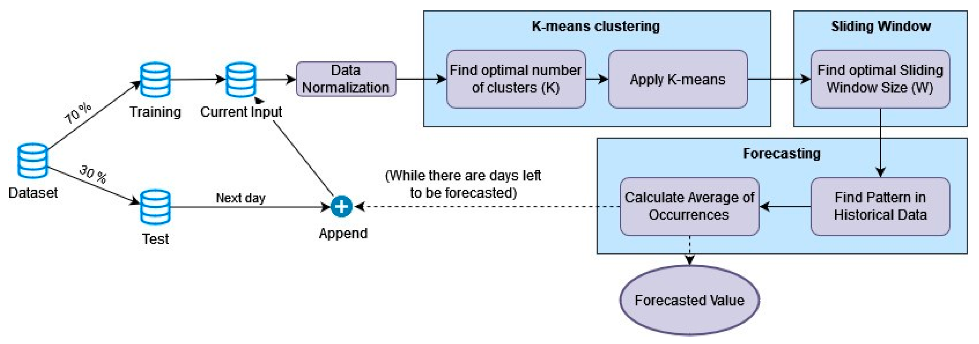
Pattern sequence-based forecasting is a general-purpose forecasting algorithm that was first proposed in 2011 [5], as illustrated in Figure 1. It is a versatile algorithm that employs clustering techniques to identify patterns in time-series data, which are subsequently used to make predictions. It is known for its efficiency and interpretability, making it a popular choice in various applications. The algorithm works as follows:

• Data normalization. The time series is standardised to reduce the effect of outliers.
• Horizon selection. The user specifies the number of consecutive observations that will be transformed into a label, and the number of observations to be forecasted in each iteration of the algorithm. This value is denoted as h, and in the context of this paper represents the number of observations per day.
• Optimal number of clusters selection. The K-means algorithm is executed for each number of clusters (K) between 2 and 15. The optimal number of clusters is selected using three different cluster validity indexes (CVI).
• Clustering/Labelling. The time series is labelled using the K-means algorithm with the optimal number of clusters.
• Optimal window size selection. We employed cross-validation to identify the optimal window size (W).
• Forecasting. The sequence of W labels corresponding to the W days before the forecasted date is searched throughout the historical data. The data from the day after the pattern is found are recorded for any occurrence, and the average of these data will produce the final forecast.
• Online learning. While there are days left to be forecasted, the last forecast ground truth is added to the training dataset and the entire process is repeated.

Improved PSF [6] is a variant of PSF that aims to reduce the training time further. Unlike the original PSF, Improved PSF utilizes only one CVI to determine the optimal number of clusters. Moreover, it does not require a sliding window for the forecasting step. Instead, the prediction is a weighted average of the cluster centers based on the frequency of each cluster per day of the week in the historical data.

SCPSNSP [7] is another variant of the previously described PSF algorithm. SCPSNSP introduces the use of Self-Organizing Maps as its main novelty, and it is the closest to our proposal. Instead of the three CVIs used by PSF, SCPSNSP uses the topographic error. The topographic error [21] measures how well the SOM preserves the topology of the input space. This is done by checking if the two best BMUs for each input are adjacent in the output map. Unlike PSF, SCPSNPS uses an ANN to predict the next sample. This ANN receives as an input signal the topographic coordinates of the symbols corresponding to the previous days (the row and column of the SOM for the previous days as numerical input) and predicts the coordinates on the topological map for the next day. Upon predicting the coordinates of a new sample, the algorithm identifies the closest cluster that contains at least one sample in it. The pattern predicted for the next day is the average of all the samples in the selected cluster.

2.5. Genetic Algorithm

A genetic algorithm [22] is an evolutionary metaheuristic inspired by Darwin’s theory of evolution. It evolves a population of potential solutions (individuals) using the concepts of fitness, selection, mutation, crossover and survival. The genetic algorithm used in this paper is described below:

• Initialization. A population with a selected number of potential solutions are initialized randomly.
• Fitness. A fitness function is used to evaluate the quality of each individual. In our case, the individual will be a set of hyperparameters of the algorithm, and the fitness function will be the Root Mean Square Error (RMSE) of the model trained with those hyperparameters.
• Selection. A random set of individuals is selected with binary tournament selection [23]. In the binary tournament, for each parent to be chosen, two individuals are selected randomly (in our case, with replacement) and put in a tournament. The winner of each tournament is the individual with the best fitness value. This individual will be selected as a parent.
• Crossover and Mutation. Each pair of parents is crossed overusing the self-adaptive binary crossover and the polynomial proposed in [24]. This will create a new set of offspring of individuals of the same size as the parent generation.
• Survival. Elitism is used to select the individuals that will conform to the next generation. This means that the next generation only keeps the individuals with the best fitness values, independent of whether they were a parent or offspring.

2.6. The Proposed Method

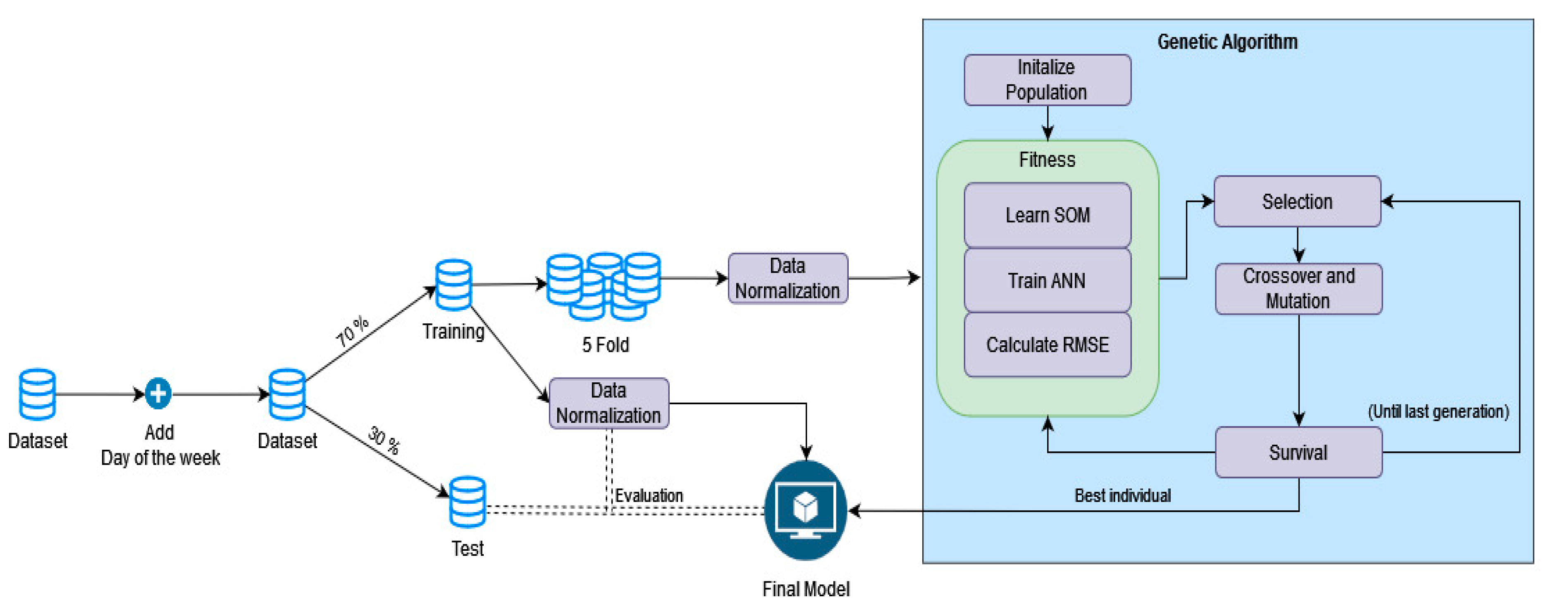
Similar to the other related proposals, our algorithm has two main steps: clustering and forecasting. However, unlike any previous proposal of this type, all hyperparameters of our algorithm are selected with a genetic algorithm. A general overview of our proposal can be found in Figure 2.

In all previously described PSF algorithms, the optimal number of clusters is selected using CVIs. The original PSF algorithm uses the silhouette index, Dunn’s index and Davies–Bouldin index; Improved PSF uses the Davies–Bouldin index; and SCPSNSP uses the topographic error. However, CVIs only measure the compactness of each cluster and the distance between different clusters. Hence, there is no guarantee that the optimal number of clusters given by any CVI will be the optimal number of clusters for the forecasting task. Therefore, in GA-SOM-NNSF, the genetic algorithm selects the optimal number of clusters (number of rows and columns of the SOM), the topology of the neural network and its learning rate. Thus, each time the genetic algorithm’s fitness function is called, a new SOM and neural network are trained according to the parameters provided by the individuals. Nevertheless, to reduce the computational overhead of training the same SOM if individuals share the same number of rows and columns of the SOM, the first time it is trained, its weights are stored on disk. The SOM is trained using the batch algorithm for up to 1000 epochs, but it can stop earlier if the BMU does not change for 3 epochs. After training, the BMU of each daily sample is assigned to a cluster identified by its row and column on the output lattice.

Afterwards, a one-hidden-layer feed-forward neural network with the sigmoid activation function in the hidden layer is used to learn the relationship between previous and future energy demand. It is well-known that using some exogenous variables can help improve the forecast. For example, the use of the temperature may help the model take into account HVAC systems, while the use of the day of the week may help the model to understand the difference in energy consumption between workdays and weekends. Nevertheless, we could not use the temperature as an exogenous variable in our study, as the datasets we used do not provide that information. This is likely due to the fact that the geographical areas we are working with are too large, and therefore, the range of temperatures for any given day may be too wide and unreliable. However, we included both days of the week and month of the year as additional features to the neural network to differentiate between loads on working days and non-working days. In our method, the neural network receives the cluster IDs from the previous X days (where X is determined by each individual of the genetic algorithm) in one-hot encoding, and the day of the week and month of the day to be predicted as exogenous variables. The output will be a unique cluster identifier in one-hot encoding. The neural network is trained for 150 epochs using the Adam optimizer with a learning rate determined by each individual of the genetic algorithm using the categorical cross-entropy loss.

While our ANN provides as output the expected cluster for a given input, both during training and to make a forecast, our method must provide a daily load for that expected cluster. The daily load of any cluster will be the weights learned by the SOM for that cluster.

Alternatives to the ANN

We opted to use an ANN in the last step of our algorithm as a one-hidden-layer feed-forward neural network can approximate any function. Furthermore, ANN has been used with success in similar approaches [7], other hybrid models [10,11] and standalone [8]. Nevertheless, this last step of our proposal could use a different machine learning model. However, linear models should be avoided, as they would be unable to learn any non-linear relationship between the input space (previous days’ cluster, day of the week and month) and the predicted clusters. If the ANN is replaced with another model, the new model’s hyperparameter should replace ANN hyperparameters (learning rate and number of hidden neurons) in the genetic algorithm.

2.7. Comparison Methodology

All algorithms were compared using the training/test partitions and the scaling method described in Section 2.1. The hyperparameters were selected automatically by using five-fold cross-validation in the training partition. We have evaluated a range of hyperparameters for each algorithm, and a maximum of 300 combinations of different parameters were tested per model. Furthermore, for reference, we evaluated two algorithms that do not involve clustering: Prophet [25] and ANN. The range of parameters considered for each method is as follows:

• PSF: Window size from 1 to 10. Number of clusters from 2 to 20;
• Improved PSF: Number of clusters from 2 to 20;
• SCPSNPS: Window size from 1 to 10. Number of rows and columns of the SOM from 5 to 10. With the Cascade-2 algorithm, resilient backpropagation and linear activation in the output layer (as described by the authors);
• GA-SOM-NNSF: Window size from 1 to 10. Number of rows and columns of the SOM from 5 to 10. Number of hidden neurons between 5 and 40. Learning rate between 0.0001 and 0.01. Population size of 15. Twenty generations;
• Prophet: Automatic parameter selection;
• ANN: Window size from 1 to 10. One hidden layer. Number of hidden layers between 5 and 40. Sigmoid activation in the hidden layer. Learning rate between 0.0001 and 0.01.

2.8. Experimental Setup

All experiments were conducted on a personal computer equipped with an AMD 5 Ryzen 2600X CPU operating at a clock speed of 3.6 GHz, an NVIDIA GeForce RTX 3060 Ti 8 GB graphics card and 32 GB of DDR4 RAM. The experiments were implemented using Python 3.9 and the libraries Simpsom [26] for the SOM, scikit-learn for K-Means and normalization, TensorFlow [27] for training neural networks, pymoo [28] for developing the genetic algorithm and FANN [29] (in C++) for the Cascade Neural Network of SCPSNSP. All random number generators were initialized with the seed value 1996. The code to execute our experiments has been provided as supplementary materials.

3. Results

3.1. Datasets’ Descriptions

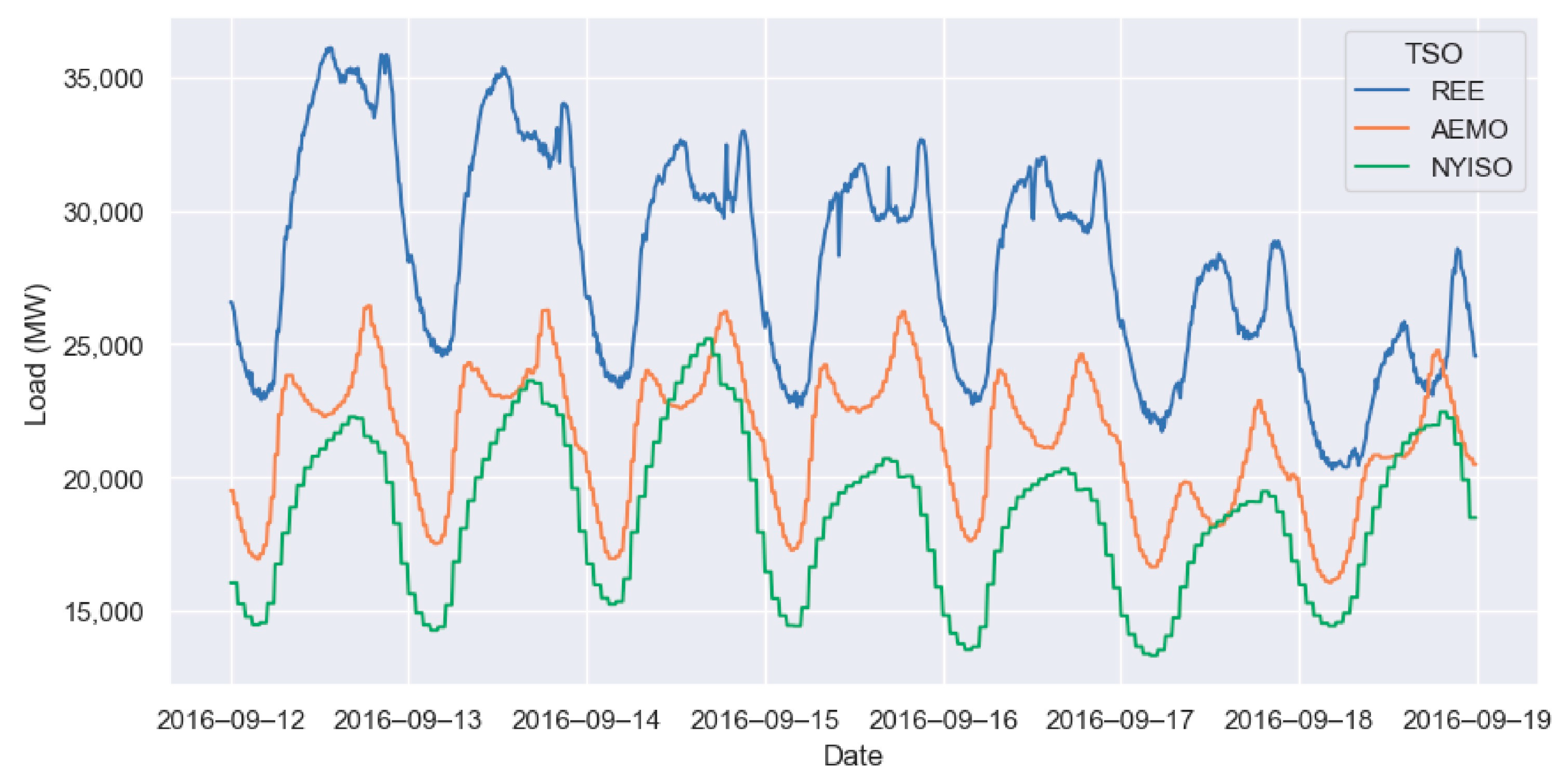
The machine learning algorithms used in this study were compared with other algorithms using the energy load data from three Transmission System Operators (TSOs). The same eleven years of data from 1 January 2009 to 31 December 2019 were taken from each dataset. Figure 3 shows a week of energy demand data from each TSO.

Red Eléctrica de España (REE) [15] is the main Spanish TSO, and its website provides information about energy demand and production in Spain since 2007, with observations recorded every 10 min. The website provides information about actual energy demand, energy demand predicted by the system, energy demand used to fix the hourly market price, energy produced by each renewable and non-renewable source, and their corresponding CO₂ emissions. However, some of these variables were gradually incorporated and may not be available for all years. The TSO system is divided into different independent subsystems for the Peninsular area, the Balearic Islands, the Canary Islands, Ceuta and Melilla. In this study, we only used data from the Peninsular area. It is important to note that the REE website does not offer a direct download of the dataset and that the data must be compiled by downloading an independent CSV file per day.

New York Independent System Operator, Inc. (NYISO) [17] is the organization responsible for managing New York State’s (USA) electric grid and its electric marketplace. Its website provides information about energy pricing, load, solar power generation and outages, among other technical reports. Most of the website’s load data have been recorded every hour. The system provides information about the entire energy load of New York State and the energy consumption in 11 different subzones of the state. For the purposes of this study, we used the aggregated energy load from the entire state of New York. The data can be obtained from the NYISO webpage, where monthly zip files are available, each containing a CSV file for every day.

Australian Energy Market Operator (AEMO) [16] is Australia’s main TSO for energy and gas. AEMO operates in two wholesale electricity markets: the National Electricity Market, operating in eastern and south-eastern Australia since 1998, and the Wholesale Electricity Market, operating in western Australia since 2006. For the purposes of this study, we used data from the National Electricity Market as they provide information about the actual load. In contrast, only the forecasted load is available for the Wholesale Electricity Market. The National Electricity Market is one of the world’s longest interconnected power systems, connecting New South Wales, the Australian Capital Territory, Queensland, South Australia, Victoria and Tasmania. The data on price and demand are provided in a single CSV file per month for each previously mentioned region, with observations recorded every 30 min. For this study, we used the aggregated demand every 30 min for all regions.

3.2. Metrics Used

Three metrics commonly used in time-series forecasting were used to evaluate the performance of each algorithm. For all these metrics, n represents the total number of observations, $\widehat{y}$ represents the predicted value, and y represents the expected value.

The Mean Absolute Percentage Error (MAPE) is a commonly used and easy-to-understand metric that provides the average difference between the forecasted and expected values in percentage. A lower MAPE value indicates a better forecast. However, MAPE can be heavily influenced by outliers and is asymmetric, meaning that overestimating and underestimating the ground truth have different effects on the metric.

$$\mathrm{M}\mathrm{A}\mathrm{P}\mathrm{E}=\frac{1}{n}{\sum }_{i=1}^n\left|\frac{y_i-\widehat{y_i}}{y_i}\right|$$

(2)

The Mean Absolute Error (MAE) is a standard metric in forecasting and regression tasks that provides the average difference between the forecasted and expected values. A lower MAE value indicates a better forecast. This metric is more robust to outliers than MAPE and RMSE.

$$\mathrm{M}\mathrm{A}\mathrm{E}=\frac{{\sum }_{i=1}^n|y_i-\widehat{y_i}|}{n}$$

(3)

The Root Mean Square Error (RMSE) is a commonly used metric in forecasting and regression tasks that measures the average difference between predicted and actual values, with a higher weight given to larger errors. A lower RMSE value indicates better performance. The RMSE metric is more useful when large errors are particularly undesirable, although it can be sensitive to outliers.

$$\mathrm{R}\mathrm{M}\mathrm{S}\mathrm{E}=\sqrt{\frac{{\sum }_{i=1}^n{\left(y_i-\widehat{y_i}\right)}^2}{n}}$$

(4)

3.3. Experimental Results

Table 1. Quality metrics obtained for REE.

Method	MAPE	MAE	RMSE	Time (s)	Best Hyperparameters
PSF	0.0639	1836.1706	2554.8588	1009.8	k = 2, w = 5
Improved PSF	0.0632	1811.2023	2350.6346	342.7	k = 2
SCPSNSP	0.0484	1368.6395	1888.6601	8534.7	5 × 5 map, w = 9
GA-SOM-NNSF	0.0362	1024.1512	1476.6051	36,300.3	7 × 10 map, w = 1, 36 neurons lr = 0.0051
Prophet	0.0554	1543.2565	2028.1925	76,948.5	Automatic
ANN	0.0236	681.7653	1010.3233	51,508.5	w = 7, lr = 0.001, 15 neurons

,

Table 2. Quality metrics obtained for AEMO.

Method	MAPE	MAE	RMSE	Time (s)	Best Hyperparameters
PSF	0.0616	1325.0971	1764.1506	933.5	k = 2, w = 4
Improved PSF	0.075	1594.5721	2020.5035	312.3	k = 2
SCPSNSP	0.049	1059.8433	1440.94	6614.3	5 × 5 map, w = 10
GA-SOM-NNSF	0.0474	1023.5576	1410.1180	14,722.2	7 × 10 map, w = 1, 33 neurons lr = 0.0084
Prophet	0.0593	1269.5846	1628.6608	25,308.6	Automatic
ANN	0.0368	797.0881	1090.1918	47,758.2	w = 10, lr = 0.0001, 20 neurons

and

Table 3. Quality metrics obtained for NYISO.

Method	MAPE	MAE	RMSE	Time (s)	Best Hyperparameters
PSF	0.0756	1355.6724	1754.3449	898.9	k = 2, w = 4
Improved PSF	0.1087	1962.0865	2475.4632	294.5	k = 2
SCPSNSP	0.0609	1098.2639	1489.5731	3503.7	6 × 6 map, w = 6
GA-SOM-NNSF	0.0522	948.7998	1294.0604	9342.7	5 × 9 map, w = 1, 36 neurons lr = 0.0053
Prophet	0.1075	1946.1666	2506.9506	21,637.5	Automatic
ANN	0.0362	667.5363	929.5423	45,838.8	w = 6, lr = 0.01, 25 neurons

present the performance of each method on the REE, AEMO and NYISO datasets. The tables report the three quality metrics’ results for the optimal model on the test partition; the total amount of time required to find the optimal hyperparameters, train the optimal model, and make the predictions; and the optimal hyperparameters for each method. Specifically, $k$ represents the optimal number of clusters for K-means, $w$ represents the window size (number of previous days to use as input) and $lr$ represents the learning rate for the neural network optimizer.

For the REE data, the ANN algorithm achieved the best performance in all three metrics, although it required a longer training time than the pattern sequence-based algorithms. On the other hand, Prophet had the slowest training time, taking more than 75,000 s, and provided only mediocre results. Among the pattern sequence-based algorithms, PSF had the worst performance, followed closely by Improved PSF. Our proposed GA-SOM-NNSF model performed considerably better than the other pattern sequence-based algorithms but required around 4.5 times more training time than SCPSNSP, although it trained 1.4 times faster than the best-performing ANN model.

For the AEMO data, the number of observations per hour was three times smaller than REE, resulting in faster training times for all algorithms. Once again, the ANN provided the best quality metrics for prediction, but it was also the slowest method to train. Prophet delivered a three-times-faster training time compared to REE, becoming the second slowest after the ANN. Unfortunately, like with the REE data, Prophet only provided better results than PSF and Improved PSF. Among the pattern sequence-based algorithms, Improved PSF provided worse results than PSF and was the worst-performing model. Our proposed method yielded the best results among pattern sequence-based algorithms. However, the improvement over SCPSNSP was relatively small compared to the difference in training time between the two, with SCPSNSP being 2.2 times faster than our proposal.

For the NYISO data, the number of observations is twice smaller than AEMO, leading to faster training for all methods. Once again, the ANN provided the best results among all the evaluated models and the improvement for having fewer observations per day in training time was marginal. Prophet was the second-slowest algorithm and provided the worst quality metrics of all algorithms, closely followed by Improved PSF. From among the pattern sequence-based algorithms, our algorithm provided the best results but was three times slower to train than SCPSNPS, the second-best algorithm of this kind.

4. Discussion

4.1. Robustness of the Approach

Before comparing the different models evaluated in this paper, we should check if our model produces robust results, i.e., the model learns without any overfitting or underfitting.

Table 4. Quality metrics for training and test with the best GA-SOM-NNSF model.

	Training				Test
Dataset	MAPE	MAE	RMSE	MAPE	MAE	RMSE
REE	0.0331	934.59	1383.56	0.0362	1024.15	1476.61
NYISO	0.0425	805.74	1164.14	0.0522	948.80	1294.06
AEMO	0.0294	663.14	975.61	0.0474	1023.56	1410.12

displays, for each dataset, the error obtained by the GA-SOM-NNSF model with the optimal hyperparameters in training and test.

The results indicate that our proposal performs well on unseen data using the REE and NYISO datasets. In both cases, the training error is a good estimator of the test error, and the difference between the two falls within reasonable boundaries as it is expected to have a slightly better result with the data used for training. However, in the case of AEMO, there is a substantial difference between the error in the training and test partitions. This does not necessarily indicate that our model is overfitting but rather that forecasting the days in the test partitions is considerably more challenging. A similar pattern can be found in the other evaluated algorithms. For example, SCPSNPS provides an RMSE of 1052.38 in the training partition and 1440.92 in the test partition.

4.2. Comparison between Algorithms

In this paper, we evaluated the performance of four pattern sequence-based forecasting algorithms (including our proposal) for energy load forecasting. The first two algorithms, PSF and Improved PSF, used K-means and averages of prior samples to produce a forecast. There were two main differences between these two algorithms. Firstly, Improved PSF only used one CVI instead of the three CVIs used by PSF. However, as seen in Table 1, Table 2 and Table 3, both methods found two to be the optimal number of clusters in all three datasets. Therefore, the main difference for all the cases studied in this paper is how each computes the prediction. As explained in Section 2.4, PSF uses a window to compute the pattern of previous days and looks for previous occurrences of that pattern. Improved PSF removes this search and calculates a weighted average of the cluster centers based on the frequency of each cluster per day of the week. While it would be expected that the inclusion of the day of the week should lead to better results, we also have to take into account that the changes made to the forecasting method may make the forecasting method less powerful, as with Improved PSF, we are completely ignoring the patterns of all the days in the history that do not share the same day of the week as the day to be forecasted. On the experiments run in this paper, Improved PSF provided slightly better results for REE but worse results for AEMO and NYISO.

The other two algorithms, SCPSNPS and our proposal, relied on using the SOM and an ANN to provide a forecast. The main difference between both was the usage of the genetic algorithm and the design of the neural network used. In SCPSNPS, the topology error is used as a CVI to obtain the optimal map size for the SOM. However, in our approach, we argue that clustering validity metrics may not always provide the optimal cluster sizes for forecasting purposes. Therefore, we employ a genetic algorithm to select the optimal cluster size and other hyperparameters for our method. The results in Table 1, Table 2 and Table 3 show that our proposal provides better results in all metrics for all three datasets at the expense of the additional training time to test a broader range of hyperparameters. The tables also display the differences between the map sizes in both algorithms, with the generic algorithm usually selecting bigger maps. This most likely indicates that even though the clustering separation or, in this case, the topology preservation may not be as good, the additional patterns provided by the new clusters can improve the forecast quality. The other main difference between both methods is the design of the neural network. In SCPSNPS, the neural network is built with a constructive algorithm and maps the coordinates between the input space and the output space. In our approach, the genetic algorithm selects the optimal hyperparameters for the neural network topology, and the mapping is performed between discrete variables representing each of the clusters. Therefore, if any exogenous variable added is also discrete, our neural network will act as a rule-based system, leading to a more straightforward interpretation once the rules are extracted. An example of a rule that could be extracted from our model would be: “If we want to predict a Friday of March and the cluster of the previous day was cluster 10, then, the next day, we expect the load profile from cluster 23”.

We also used two non-PSF algorithms to compare the results: Prophet and the ANN. Both models were slower to train than the PSF algorithms in all datasets, as expected. Prophet did not provide great results in any of the three datasets evaluated. However, the ANN always provided better metrics at the expense of being the slowest method to train. This differs from the results reported in the original PSF algorithms papers, but it could be explained by the improvements made in optimizers and weight initialization strategies over the last decade, and the larger amount of data used to train the neural networks could also explain the difference.

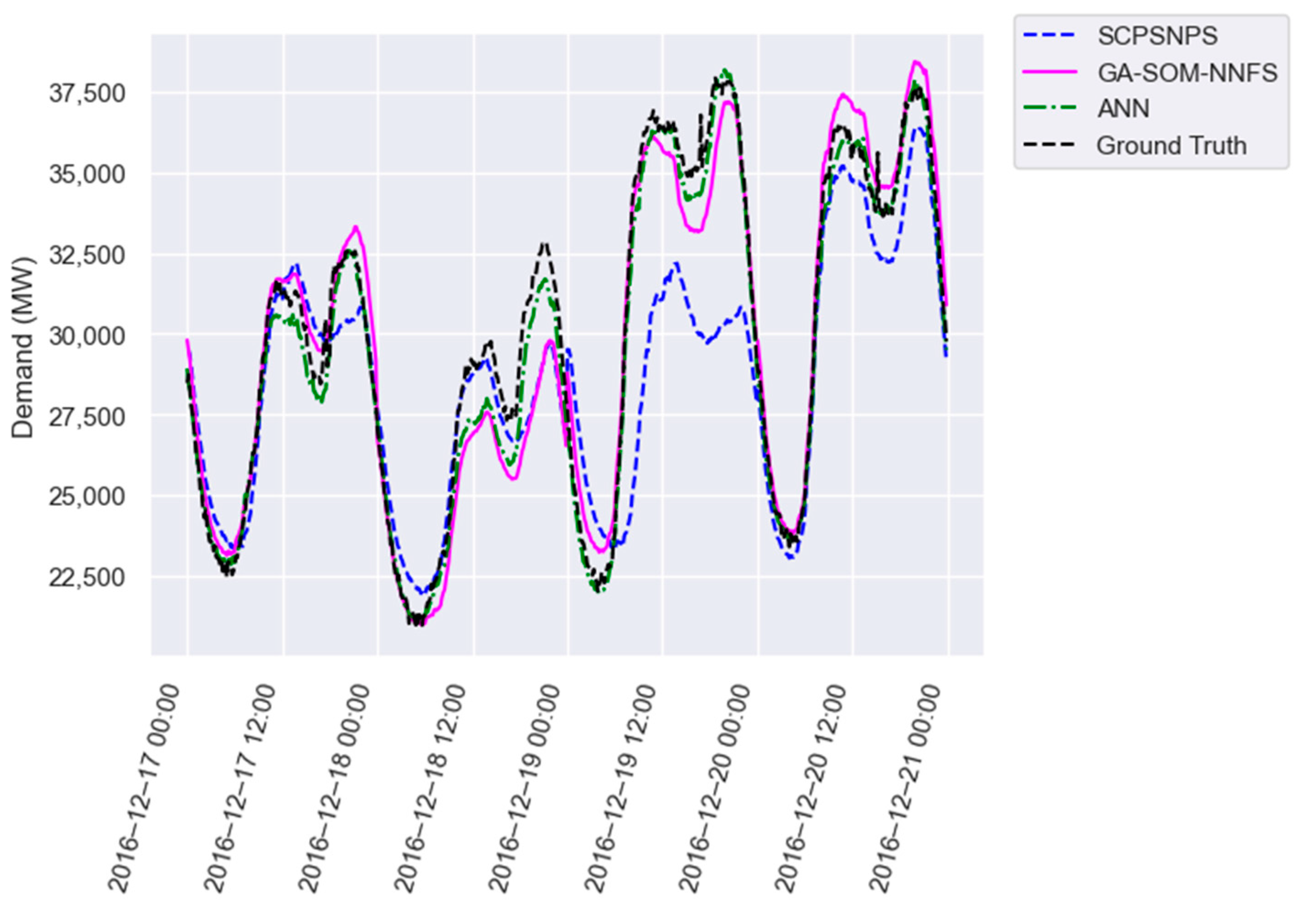
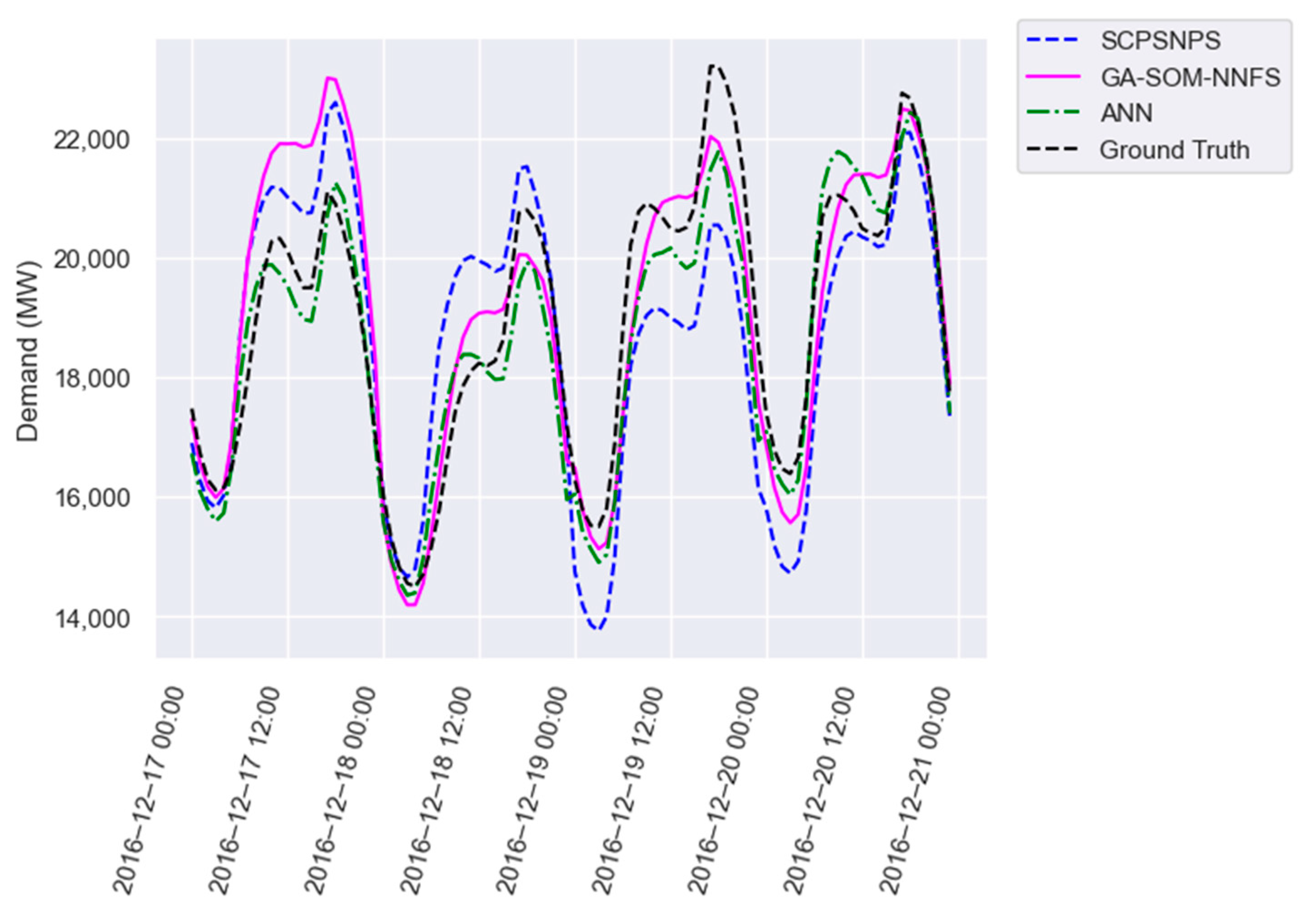
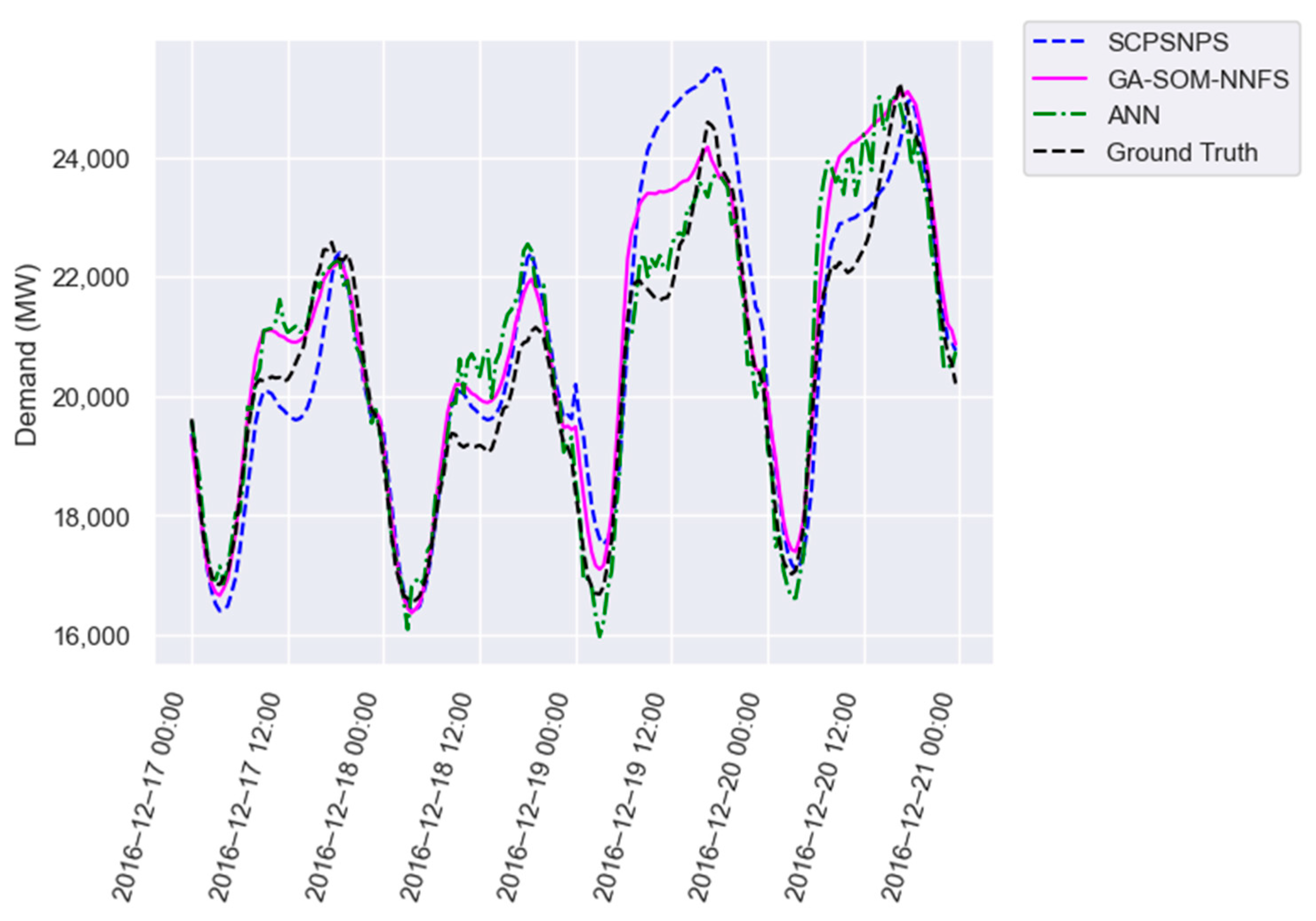
Figure 4, Figure 5 and Figure 6 provide a visual comparison of the forecast provided by SCPSNPS (blue), our proposal (pink) and the artificial neural network (green) with the expected value (black) for four consecutive days of test partition in all three datasets. In all three figures, the ANN provided a better forecast than the PSF algorithms, although there were some days when the PSF algorithms provided a more accurate approximation. Between GA-SOM-NNFS and our proposal, there were days when one offered better results than the other and vice versa. However, it was more frequent for SCPSNPS to use patterns significantly different from the closest possible pattern, as observed on the third day of each plot.

4.3. Practical Applications of the Proposed Algorithm

Even though our algorithm provided better results than all other pattern sequence-based algorithms, the ANN consistently outperformed our proposed algorithm in terms of accuracy, though requiring more training time. Therefore, in scenarios where accuracy is the primary concern, ANNs should be preferred over our proposed algorithm. However, if there are any limitations to the amount of time available to train the models, our proposal (or any other pattern sequence-based algorithm) should be used, although it is also computationally expensive. In those scenarios, the genetic algorithm could stop prematurely if the time restriction was reached, providing the best forecast for the time available to train. This could be further improved with parallel or distributed versions of the algorithm, drastically reducing the time required to train the SOMs and run the genetic algorithm.

Another significant advantage of our approach is its high interpretability. In this case, if the SOM finds an interesting pattern (or the pattern of interest is artificially introduced in the SOM), the ANN will learn relationships between that pattern, previous days’ patterns, the day of the week and the month. Due to the discrete nature of all input and output data, simple understandable rules could be easily extracted from the ANN, providing experts with better insights into why that pattern was occurring.

5. Conclusions

The work presented in this paper had two main goals: first, to evaluate different pattern sequence-based algorithms using large amounts of data, and second, to develop an algorithm that challenges the idea of using a CVI to determine the optimal cluster size in forecasting tasks.

To evaluate the pattern sequence-based algorithms, we used three publicly available data sources of energy demand with ten years of data recorded at an hourly and sub-hourly granularity. This is in contrast to previous studies that used only one dataset or less than two years of data. While pattern sequence-based algorithms had provided incredible results in energy demand in previous studies, our results showed that Artificial Neural Networks provided more accurate results, but they required more training time.

The second goal of our research was to develop an improved pattern sequence-based algorithm to address some of the weak points of previous proposals. The major difference in our proposal was the use of a genetic algorithm to select the optimal cluster size and the other neural network hyperparameters instead of using a cluster validity index. Our proposal provided better forecasts than all other pattern sequence-based algorithms but was also the slowest among them due to the use of the genetic algorithm. The optimal cluster sizes provided by our algorithm were completely different from those offered by the Cluster Validity Index used in the other proposal that makes use of the Self-Organizing Map, indicating that a Cluster Validity Index is most likely not the best tool to select clustering hyperparameters when the actual objective is to produce an accurate forecast.

In future works, we propose studying adaptations of our proposal for parallel and distributed architectures to reduce training time and evaluating pattern sequence-based algorithms in ensembles with other time-series forecasting algorithms.