


Image Fundus Classification System for Diabetic Retinopathy Stage Detection Using Hybrid CNN-DELM

 ,
,  , ,
, ,  and
and
Abstract
1. Introduction
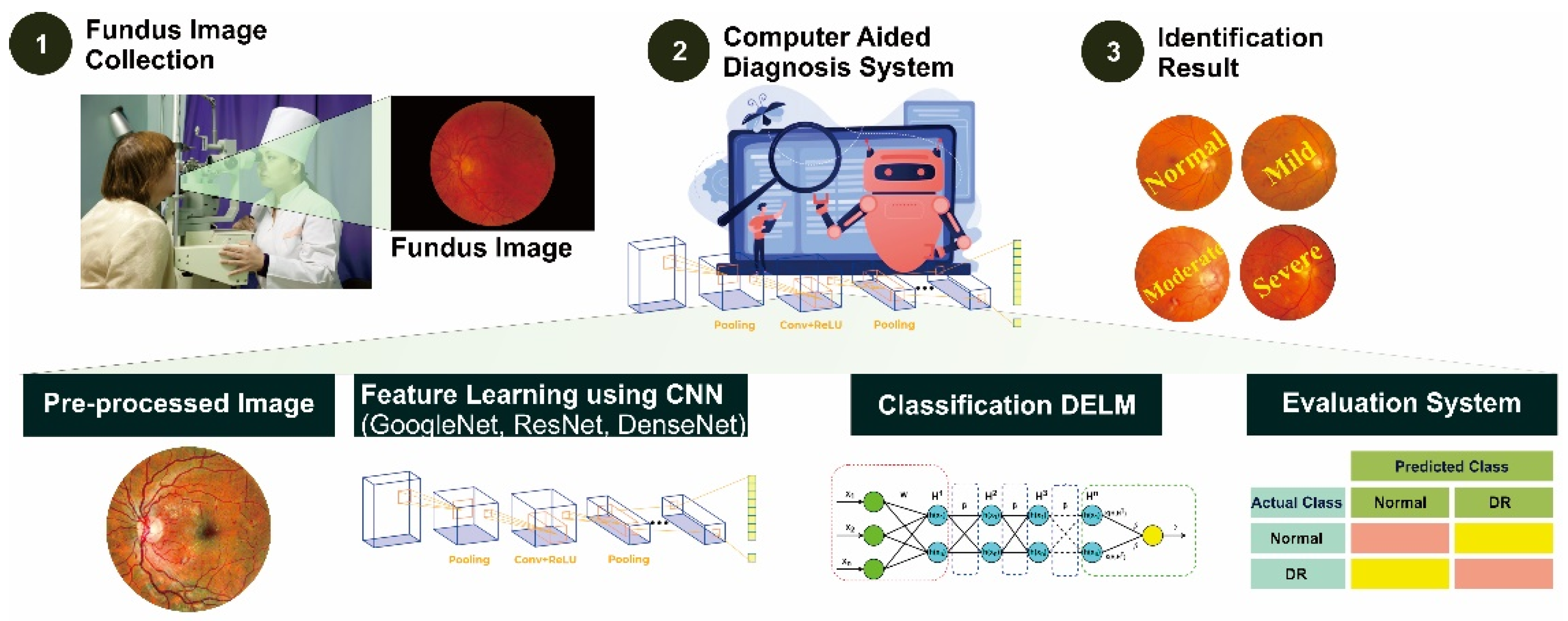
2. Materials and Methods
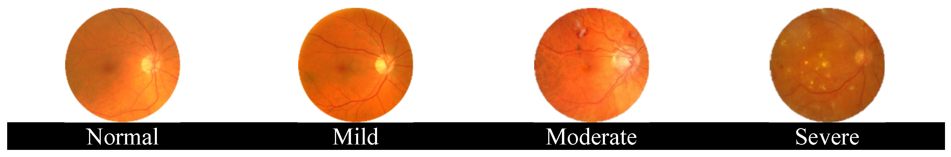
2.1. Diabetic Retinopathy
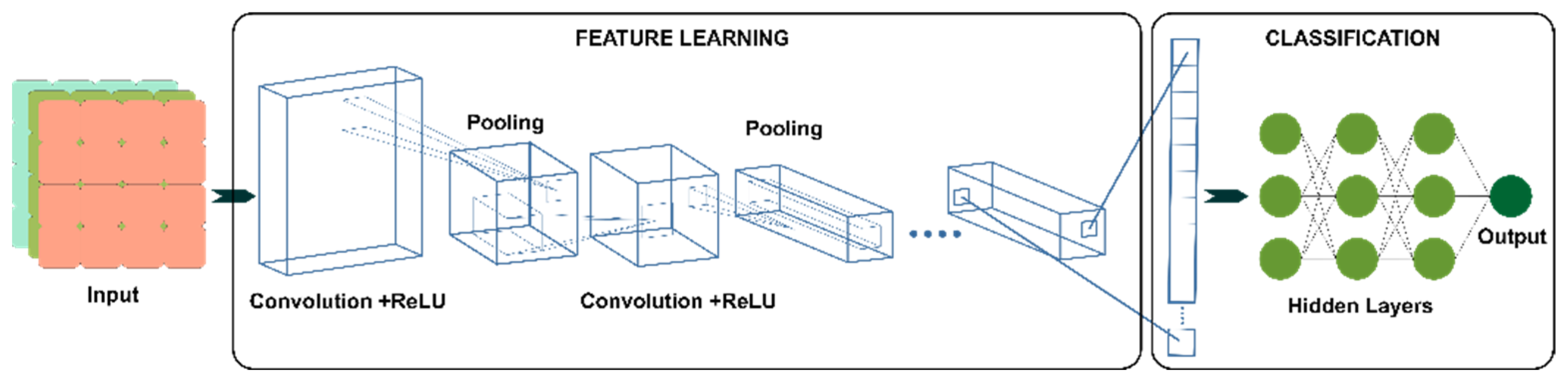
2.2. Convolutional Neural Network
2.2.1. GoogleNet
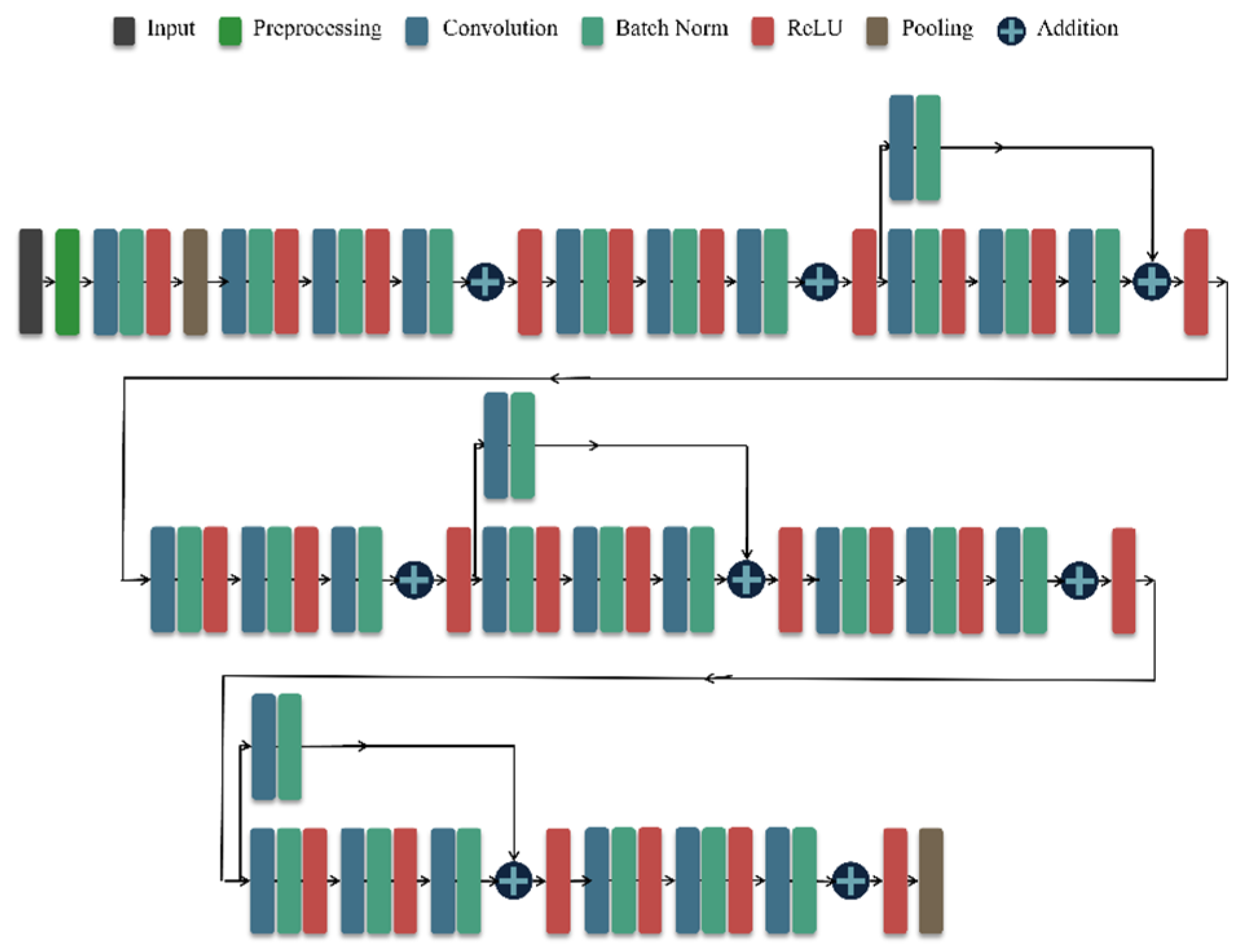
2.2.2. ResNet
2.2.3. DenseNet
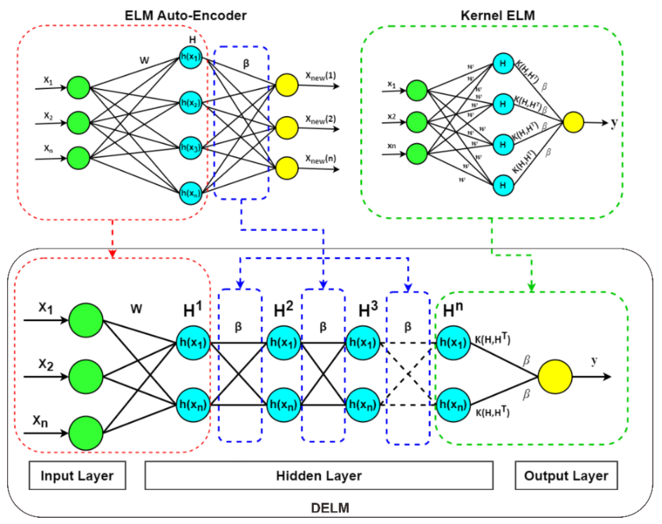
2.3. Deep Extreme Learning Machine (DELM)
3. Results
4. Conclusions
Author Contributions
Funding
Data Availability Statement
Conflicts of Interest
References
- Cheloni, R.; Gandolfi, S.A.; Signorelli, C.; Odone, A. Global Prevalence of Diabetic Retinopathy: Protocol for a Systematic Review and Meta-Analysis. BMJ Open 2019, 9, 2015–2019. [Google Scholar] [CrossRef] [PubMed]
- Wang, W.; Lo, A.C.Y. Diabetic Retinopathy: Pathophysiology and Treatments. Int. J. Mol. Sci. 2018, 19, 1816. [Google Scholar] [CrossRef] [PubMed]
- Lima, V.C.; Cavalieri, G.C.; Lima, M.C.; Nazario, N.O.; Lima, G.C. Risk Factors for Diabetic Retinopathy: A Case-Control Study. Int. J. Retin. Vitr. 2016, 2, 21. [Google Scholar] [CrossRef]
- Ren, C.; Liu, W.; Li, J.; Cao, Y.; Xu, J.; Lu, P. Physical Activity and Risk of Diabetic Retinopathy: A Systematic Review and Meta-Analysis. Acta Diabetol. 2019, 56, 823–837. [Google Scholar] [CrossRef] [PubMed]
- Porwal, P.; Pachade, S.; Kamble, R.; Kokare, M.; Deshmukh, G.; Sahasrabuddhe, V.; Meriaudeau, F. Indian Diabetic Retinopathy Image Dataset (IDRiD): A Database for Diabetic Retinopathy Screening Research. Data 2018, 3, 25. [Google Scholar] [CrossRef]
- Bellemo, V.; Lim, G.; Rim, T.H.; Tan, G.S.W.; Cheung, C.Y.; Sadda, S.; He, M.; Tufail, A.; Lee, M.L.; Hsu, W. Artificial Intelligence Screening for Diabetic Retinopathy: The Real-World Emerging Application. Curr. Diab. Rep. 2019, 19, 72. [Google Scholar] [CrossRef] [PubMed]
- Mansour, R.F. Deep-Learning-Based Automatic Computer-Aided Diagnosis System for Diabetic Retinopathy. Biomed. Eng. Lett. 2018, 8, 41–57. [Google Scholar] [CrossRef]
- Asyhar, A.H.; Foeady, A.Z.; Thohir, M.; Arifin, A.Z.; Haq, D.Z.; Novitasari, D.C.R. Implementation LSTM Algorithm for Cervical Cancer Using Colposcopy Data. In Proceedings of the 2020 International Conference on Artificial Intelligence in Information and Communication (ICAIIC), Fukuoka, Japan, 19–21 February 2020; pp. 485–489. [Google Scholar]
- Foeady, A.Z.; Novitasari, D.C.R.; Asyhar, A.H.; Firmansjah, M. Automated Diagnosis System of Diabetic Retinopathy Using GLCM Method and SVM Classifier. Proceeding Electr. Eng. Comput. Sci. Inform. 2018, 5, 154–160. [Google Scholar]
- Bora, M.B.; Daimary, D.; Amitab, K.; Kandar, D. Handwritten Character Recognition from Images Using CNN-ECOC. Procedia Comput. Sci. 2020, 167, 2403–2409. [Google Scholar] [CrossRef]
- Chakrabarty, N. A Deep Learning Method for the Detection of Diabetic Retinopathy. In Proceedings of the 2018 5th IEEE Uttar Pradesh Section International Conference on Electrical, Electronics and Computer Engineering (UPCON), Gorakhpur, India, 2–4 November 2018; pp. 1–5. [Google Scholar] [CrossRef]
- Shanthi, T.; Sabeenian, R.S. Modified Alexnet Architecture for Classification of Diabetic Retinopathy Images. Comput. Electr. Eng. 2019, 76, 56–64. [Google Scholar] [CrossRef]
- Anand, R.; Shanthi, T.; Nithish, M.S.; Lakshman, S. Face Recognition and Classification Using GoogleNET Architecture. In Soft Computing for Problem Solving; Springer: Berlin/Heidelberg, Germany, 2020; pp. 261–269. [Google Scholar]
- Mahajan, A.; Chaudhary, S. Categorical Image Classification Based on Representational Deep Network (RESNET). In Proceedings of the 2019 3rd International conference on Electronics, Communication and Aerospace Technology (ICECA), Coimbatore, India, 12–14 June 2019; pp. 327–330. [Google Scholar] [CrossRef]
- Li, H.; Zhuang, S.; Li, D.; Zhao, J.; Ma, Y. Benign and Malignant Classification of Mammogram Images Based on Deep Learning. Biomed. Signal Process. Control 2019, 51, 347–354. [Google Scholar] [CrossRef]
- Xu, K.; Feng, D.; Mi, H. Deep Convolutional Neural Network-Based Early Automated Detection of Diabetic Retinopathy Using Fundus Image. Molecules 2017, 22, 2054. [Google Scholar] [CrossRef] [PubMed]
- dos Santos, M.M.; da Silva Filho, A.G.; dos Santos, W.P. Deep Convolutional Extreme Learning Machines: Filters Combination and Error Model Validation. Neurocomputing 2019, 329, 359–369. [Google Scholar] [CrossRef]
- Pang, S.; Yang, X. Deep Convolutional Extreme Learning Machine and Its Application in Handwritten Digit Classification. Comput. Intell. Neurosci. 2016, 2016, 3049632. [Google Scholar] [CrossRef] [PubMed]
- Yin, Y.; Li, H.; Wen, X. Multi-Model Convolutional Extreme Learning Machine with Kernel for RGB-D Object Recognition. In Proceedings of the LIDAR Imaging Detection and Target Recognition 2017, Changchun, China, 23–25 July 2017. International Society for Optics and Photonics. [Google Scholar]
- Xiao, D.; Li, B.; Mao, Y. A Multiple Hidden Layers Extreme Learning Machine Method and Its Application. Math. Probl. Eng. 2017, 2017, 4670187. [Google Scholar] [CrossRef]
- Tissera, M.D.; McDonnell, M.D. Deep Extreme Learning Machines: Supervised Autoencoding Architecture for Classification. Neurocomputing 2016, 174, 42–49. [Google Scholar] [CrossRef]
- Uzair, M.; Shafait, F.; Ghanem, B.; Mian, A. Representation Learning with Deep Extreme Learning Machines for Efficient Image Set Classification. Neural Comput. Appl. 2018, 30, 1211–1223. [Google Scholar] [CrossRef]
- Ding, S.; Zhang, N.; Xu, X.; Guo, L.; Zhang, J. Deep Extreme Learning Machine and Its Application in EEG Classification. Math. Probl. Eng. 2015, 2015, 129021. [Google Scholar] [CrossRef]
- Omar, Z.A.; Hanafi, M.; Mashohor, S.; Mahfudz, N.F.M.; Muna’Im, M. Automatic Diabetic Retinopathy Detection and Classification System. In Proceedings of the 2017 7th IEEE International Conference on System Engineering and Technology (ICSET), Shah Alam, Malaysia, 2–3 October 2017; pp. 162–166. [Google Scholar] [CrossRef]
- Faust, O.; Acharya, R.; Ng, E.Y.-K.; Ng, K.-H.; Suri, J.S. Algorithms for the Automated Detection of Diabetic Retinopathy Using Digital Fundus Images: A Review. J. Med. Syst. 2012, 36, 145–157. [Google Scholar] [CrossRef]
- Hassan, S.A.; Akbar, S.; Rehman, A.; Saba, T.; Kolivand, H.; Bahaj, S.A. Recent Developments in Detection of Central Serous Retinopathy Through Imaging and Artificial Intelligence Techniques—A Review. IEEE Access 2021, 9, 168731–168748. [Google Scholar] [CrossRef]
- Spencer, B.G.; Estevez, J.J.; Liu, E.; Craig, J.E.; Finnie, J.W. Pericytes, Inflammation, and Diabetic Retinopathy. Inflammopharmacology 2020, 28, 697–709. [Google Scholar] [CrossRef] [PubMed]
- Zaki, W.M.D.W.; Zulkifley, M.A.; Hussain, A.; Halim, W.H.W.A.; Mustafa, N.B.A.; Ting, L.S. Diabetic Retinopathy Assessment: Towards an Automated System. Biomed. Signal Process. Control 2016, 24, 72–82. [Google Scholar] [CrossRef]
- Cai, X.; McGinnis, J.F. Diabetic Retinopathy: Animal Models, Therapies, and Perspectives. J. Diabetes Res. 2016, 2016, 3789217. [Google Scholar] [CrossRef] [PubMed]
- Dorj, U.O.; Lee, K.K.; Choi, J.Y.; Lee, M. The Skin Cancer Classification Using Deep Convolutional Neural Network. Multimed. Tools Appl. 2018, 77, 9909–9924. [Google Scholar] [CrossRef]
- Ker, J.; Wang, L.; Rao, J.; Lim, T. Deep Learning Applications in Medical Image Analysis. IEEE Access 2017, 6, 9375–9379. [Google Scholar] [CrossRef]
- Nguyen, H.T.; Lee, E.H.; Lee, S. Study on the Classification Performance of Underwater Sonar Image Classification Based on Convolutional Neural Networks for Detecting a Submerged Human Body. Sensors 2020, 20, 94. [Google Scholar] [CrossRef]
- Yamashita, R.; Nishio, M.; Do, R.K.G.; Togashi, K. Convolutional Neural Networks: An Overview and Application in Radiology. Insights Imaging 2018, 9, 611–629. [Google Scholar] [CrossRef]
- Saba, T.; Akbar, S.; Kolivand, H.; Ali Bahaj, S. Automatic Detection of Papilledema through Fundus Retinal Images Using Deep Learning. Microsc. Res. Tech. 2021, 84, 3066–3077. [Google Scholar] [CrossRef]
- Chauhan, R.; Ghanshala, K.K.; Joshi, R.C. Convolutional Neural Network (CNN) for Image Detection and Recognition. In Proceedings of the 2018 First International Conference on Secure Cyber Computing and Communication (ICSCCC), Jalandhar, India, 15–17 December 2018; pp. 278–282. [Google Scholar]
- Wang, S.H.; Phillips, P.; Sui, Y.; Liu, B.; Yang, M.; Cheng, H. Classification of Alzheimer’s Disease Based on Eight-Layer Convolutional Neural Network with Leaky Rectified Linear Unit and Max Pooling. J. Med. Syst. 2018, 42, 85. [Google Scholar] [CrossRef]
- Qomariah, D.U.N.; Tjandrasa, H.; Fatichah, C. Classification of Diabetic Retinopathy and Normal Retinal Images Using CNN and SVM. In Proceedings of the 2019 12th International Conference on Information & Communication Technology and System (ICTS), Surabaya, Indonesia, 18 July 2019; pp. 152–157. [Google Scholar] [CrossRef]
- Zhang, X.; Pan, W.; Bontozoglou, C.; Chirikhina, E.; Chen, D.; Xiao, P. Skin Capacitive Imaging Analysis Using Deep Learning GoogLeNet; Springer International Publishing: Berlin/Heidelberg, Germany, 2020; Volume 1229, AISC; ISBN 9783030522452. [Google Scholar]
- Zmudzinski, L. Deep Learning Guinea Pig Image Classification Using NVIDIA DIGITS and GoogLeNet. CEUR Workshop Proc. 2018, 2240, 5. [Google Scholar]
- Smith, D. Comparison of Google Image Search and ResNet Image Classification Using Image Similarity Metrics. Bachelor’s Thesis, University of Arkansas, Fayetteville, Arkansas, 2018. [Google Scholar]
- Kumar, A.; Kalia, A. Object Classification: Performance Evaluation of Cnn Based Classifiers Using Standard Object Detection Datasets. Int. J. Adv. Sci. Technol. 2019, 28, 135–143. [Google Scholar]
- Qin, J.; Pan, W.; Xiang, X.; Tan, Y.; Hou, G. A Biological Image Classification Method Based on Improved CNN. Ecol. Inform. 2020, 58, 101093. [Google Scholar] [CrossRef]
- Huang, G.B.; Zhu, Q.Y.; Siew, C.K. Extreme Learning Machine: A New Learning Scheme of Feedforward Neural Networks. IEEE Int. Conf. Neural Networks-Conf. Proc. 2004, 2, 985–990. [Google Scholar] [CrossRef]
- Ibrahim, W.; Abadeh, M.S. Extracting Features from Protein Sequences to Improve Deep Extreme Learning Machine for Protein Fold Recognition. J. Theor. Biol. 2017, 421, 1–15. [Google Scholar] [CrossRef] [PubMed]
- Yamin Siddiqui, S.; Adnan Khan, M.; Abbas, S.; Khan, F. Smart Occupancy Detection for Road Traffic Parking Using Deep Extreme Learning Machine. J. King Saud Univ.—Comput. Inf. Sci. 2020, 34, 727–733. [Google Scholar] [CrossRef]
- Khan, S.H.; Abbas, Z.; Rizvi, S.M.D. Classification of Diabetic Retinopathy Images Based on Customised CNN Architecture. In Proceedings of the 2019 Amity International Conference on Artificial Intelligence (AICAI), Dubai, United Arab Emirates, 4–6 February 2019; pp. 244–248. [Google Scholar]
- Hua, C.-H.; Huynh-The, T.; Lee, S. Retinal Vessel Segmentation Using Round-Wise Features Aggregation on Bracket-Shaped Convolutional Neural Networks. In Proceedings of the 2019 41st Annual International Conference of the IEEE Engineering in Medicine and Biology Society (EMBC), Berlin, Germany, 23–27 July 2019; pp. 36–39. [Google Scholar]


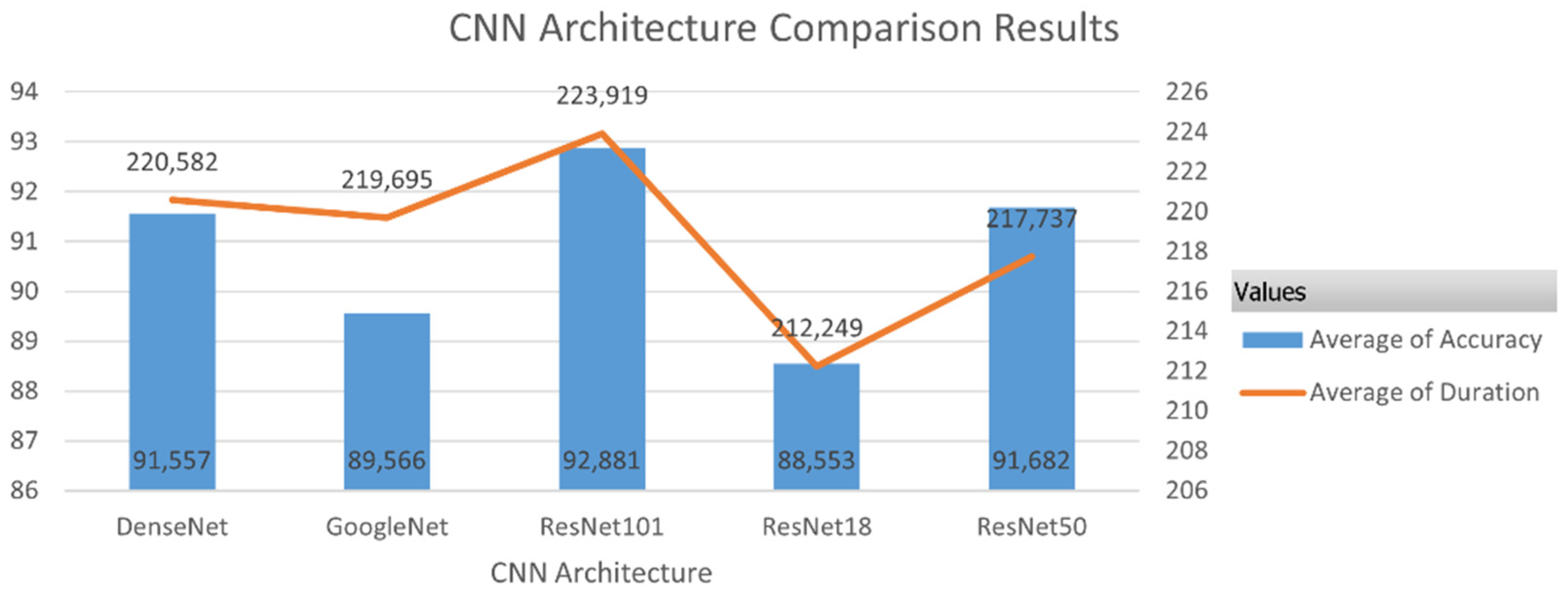
| No Feature | GoogleNet | ResNet18 | ResNet50 | ResNet101 | DenseNet |
|---|---|---|---|---|---|
| 1 | 0.0500 | 1.2727 | 3.1410 | 2.0698 | −0.0001 |
| 2 | 0.2205 | 1.7893 | 0.0496 | 0 | 0.0004 |
| 3 | 0 | 0.3892 | 0 | 0.0629 | 0.0018 |
| 4 | 0.5618 | 0.2355 | 0.1208 | 0 | −0.0963 |
| 5 | 0.0173 | 0.1450 | 0.0105 | 0.1196 | 0.0022 |
| 6 | 0.0241 | 0.6516 | 0 | 0.4925 | 0.0002 |
| 7 | 0 | 0.3554 | 0.0048 | 1.5753 | −0.0004 |
| 8 | 0 | 1.0218 | 0.2059 | 0.1258 | 0.0007 |
| 9 | 0.0268 | 1.3834 | 0 | 0.3570 | 0.0002 |
| 10 | 0.1011 | 0.7051 | 0.1300 | 0.5861 | 0.0090 |
| feature-n | 0.4129 | 0.0715 | 0.3104 | 0.4698 | 0.8898 |
| Total feature | 1024 | 512 | 2048 | 2048 | 1920 |
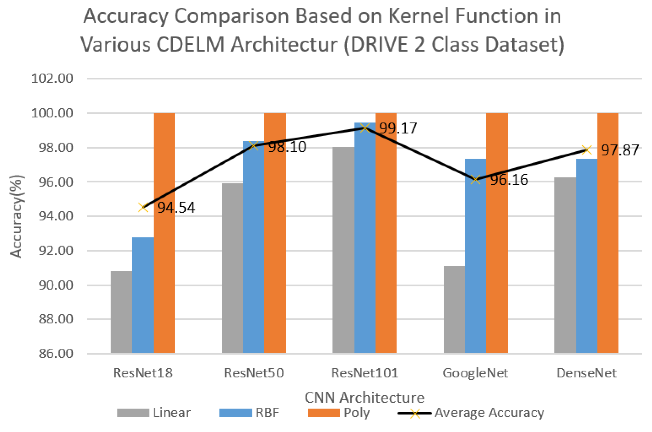
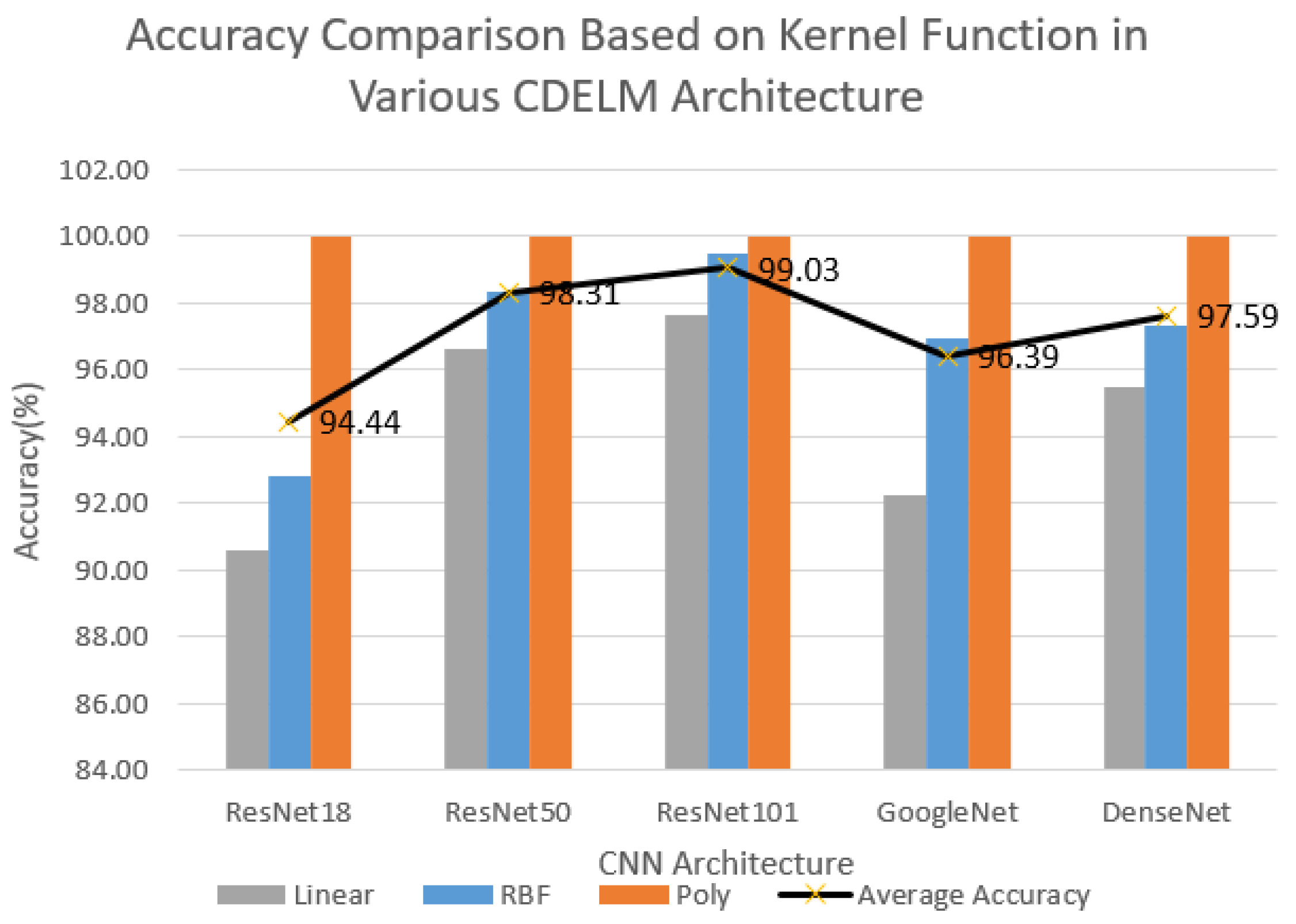
| CNN Architecture | Kernel | Accuracy (%) | Sensitivity (%) | Specificity (%) | Duration (s) |
|---|---|---|---|---|---|
| ResNet18 | Linear | 90.83 | 90.83 | 90.97 | 288.50 |
| RBF | 92.78 | 92.78 | 92.92 | 288.10 | |
| Poly | 100.00 | 100.00 | 100.00 | 291.22 | |
| ResNet50 | Linear | 95.90 | 95.90 | 96.21 | 299.17 |
| RBF | 98.40 | 98.40 | 98.45 | 295.58 | |
| Poly | 100.00 | 100.00 | 100.00 | 295.37 | |
| ResNet101 | Linear | 98.06 | 98.06 | 98.12 | 296.63 |
| RBF | 99.44 | 99.44 | 99.45 | 300.62 | |
| Poly | 100.00 | 100.00 | 100.00 | 298.02 | |
| GoogleNet | Linear | 91.11 | 91.11 | 91.92 | 300.24 |
| RBF | 97.36 | 97.36 | 97.45 | 299.29 | |
| Poly | 100.00 | 100.00 | 100.00 | 307.13 | |
| DenseNet | Linear | 96.25 | 96.25 | 96.35 | 302.45 |
| RBF | 97.36 | 97.36 | 97.49 | 328.36 | |
| Poly | 100.00 | 100.00 | 100.00 | 306.15 |
| CNN Architecture | Kernel | Accuracy (%) | Sensitivity (%) | Specificity (%) | Duration (s) |
|---|---|---|---|---|---|
| ResNet18 | Linear | 90.56 | 90.56 | 90.72 | 290.25 |
| RBF | 92.78 | 92.78 | 92.92 | 284.36 | |
| Poly | 100.00 | 100.00 | 100.00 | 287.24 | |
| ResNet50 | Linear | 96.60 | 96.60 | 96.78 | 293.76 |
| RBF | 98.33 | 98.33 | 98.38 | 291.99 | |
| Poly | 100.00 | 100.00 | 100.00 | 294.61 | |
| ResNet101 | Linear | 97.64 | 97.64 | 97.72 | 298.70 |
| RBF | 99.44 | 99.44 | 99.45 | 293.67 | |
| Poly | 100.00 | 100.00 | 100.00 | 293.08 | |
| GoogleNet | Linear | 92.22 | 92.22 | 92.86 | 294.98 |
| RBF | 96.94 | 96.94 | 97.06 | 288.39 | |
| Poly | 100.00 | 100.00 | 100.00 | 290.46 | |
| DenseNet | Linear | 95.49 | 95.49 | 95.62 | 298.19 |
| RBF | 97.29 | 97.29 | 97.43 | 290.27 | |
| Poly | 100.00 | 100.00 | 100.00 | 289.96 |
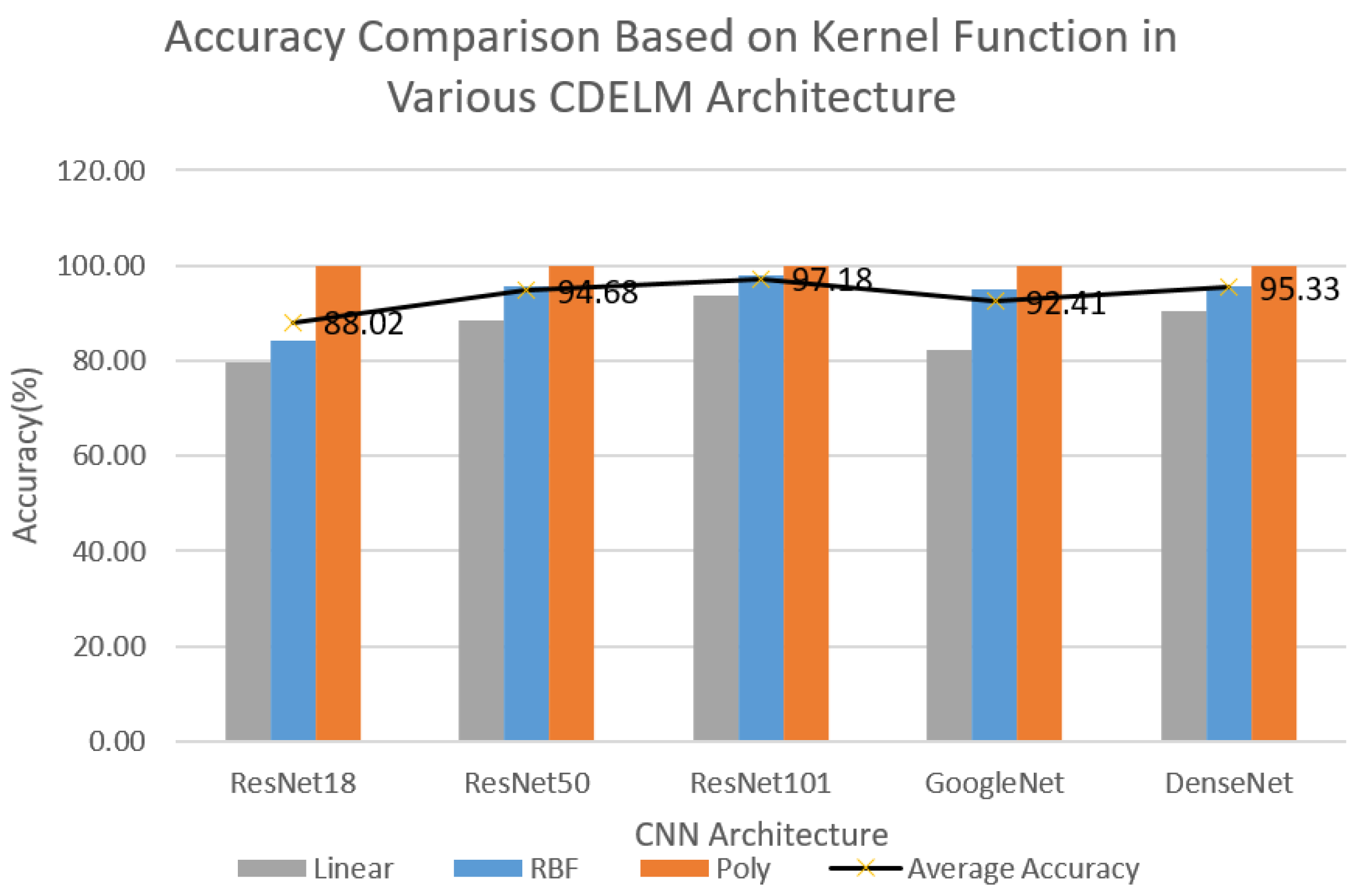
| CNN Architecture | Kernel | Accuracy (%) | Sensitivity (%) | Specificity (%) | Duration (s) |
|---|---|---|---|---|---|
| ResNet18 | Linear | 79.72 | 79.72 | 79.85 | 136.04 |
| RBF | 84.33 | 84.33 | 84.33 | 135.43 | |
| Poly | 100.00 | 100.00 | 100.00 | 140.27 | |
| ResNet50 | Linear | 88.52 | 88.52 | 88.83 | 136.95 |
| RBF | 95.51 | 95.51 | 95.63 | 138.10 | |
| Poly | 100.00 | 100.00 | 100.00 | 146.84 | |
| ResNet101 | Linear | 93.55 | 93.55 | 93.63 | 137.25 |
| RBF | 98.00 | 98.00 | 98.00 | 138.84 | |
| Poly | 100.00 | 100.00 | 100.00 | 142.72 | |
| GoogleNet | Linear | 82.11 | 82.11 | 82.29 | 136.07 |
| RBF | 95.12 | 95.12 | 95.18 | 138.04 | |
| Poly | 100.00 | 100.00 | 100.00 | 141.78 | |
| DenseNet | Linear | 90.52 | 90.52 | 90.60 | 138.41 |
| RBF | 95.47 | 95.47 | 95.46 | 138.37 | |
| Poly | 100.00 | 100.00 | 100.00 | 140.99 |
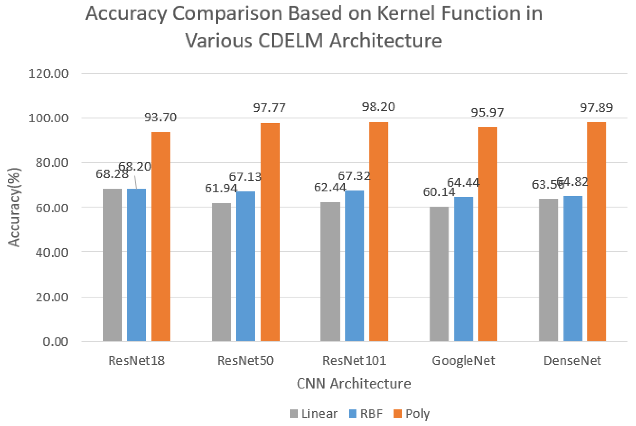
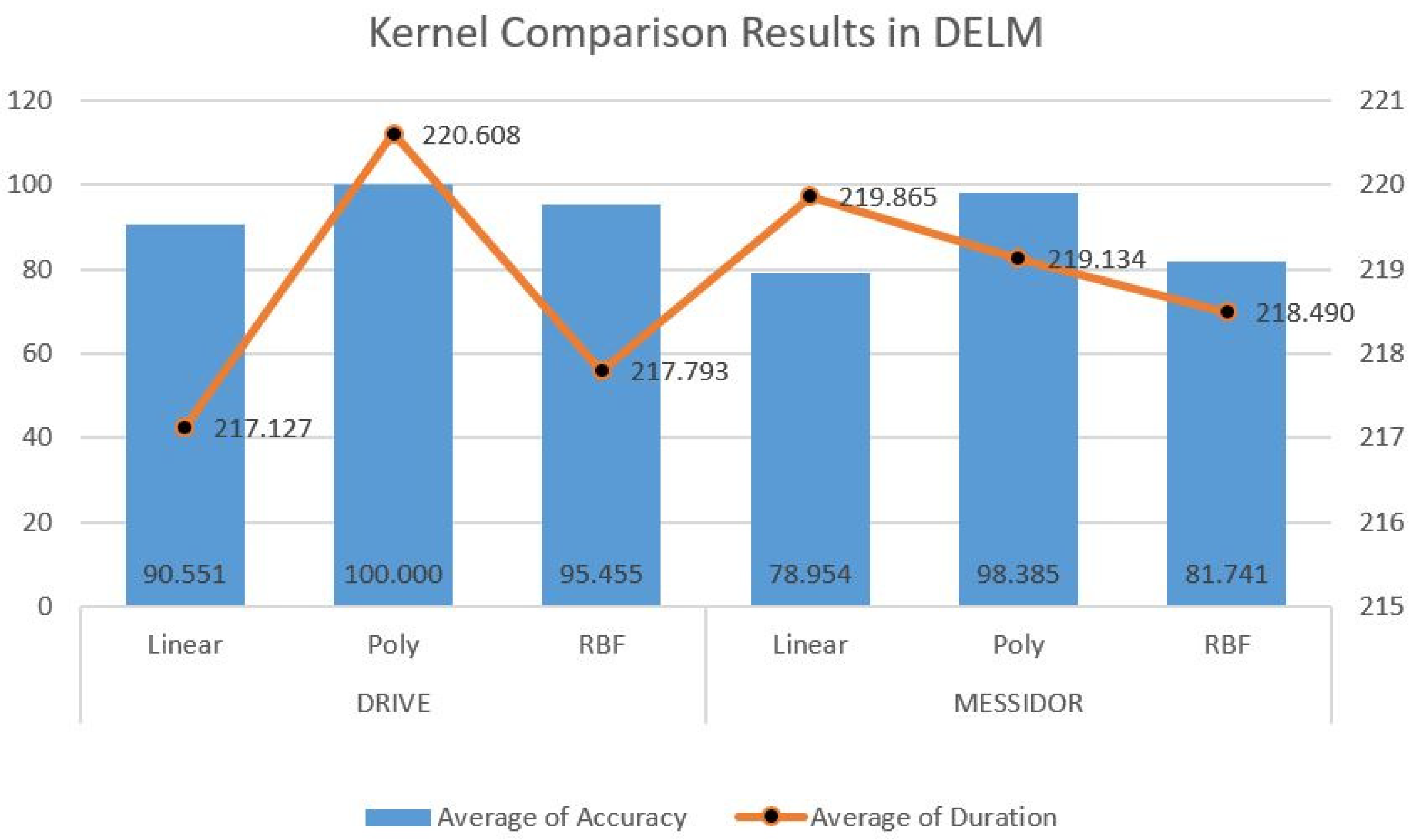
| CNN Architecture | Kernel | Accuracy (%) | Sensitivity (%) | Specificity (%) | Duration (s) |
|---|---|---|---|---|---|
| ResNet18 | Linear | 68.28 | 68.28 | 69.11 | 137.21 |
| RBF | 68.20 | 68.20 | 67.72 | 138.00 | |
| Poly | 93.70 | 93.70 | 93.70 | 143.55 | |
| ResNet50 | Linear | 61.94 | 61.94 | 61.05 | 139.06 |
| RBF | 67.13 | 67.13 | 66.58 | 144.96 | |
| Poly | 97.77 | 97.77 | 97.77 | 144.78 | |
| ResNet101 | Linear | 62.44 | 62.44 | 62.44 | 159.63 |
| RBF | 67.32 | 67.32 | 67.10 | 161.81 | |
| Poly | 98.20 | 98.20 | 98.19 | 166.94 | |
| GoogleNet | Linear | 60.14 | 60.14 | 59.36 | 161.97 |
| RBF | 64.44 | 64.44 | 64.19 | 140.73 | |
| Poly | 95.97 | 95.97 | 96.03 | 144.16 | |
| DenseNet | Linear | 63.56 | 63.56 | 63.17 | 137.56 |
| RBF | 64.82 | 64.82 | 64.39 | 162.28 | |
| Poly | 97.89 | 97.89 | 97.90 | 142.77 |
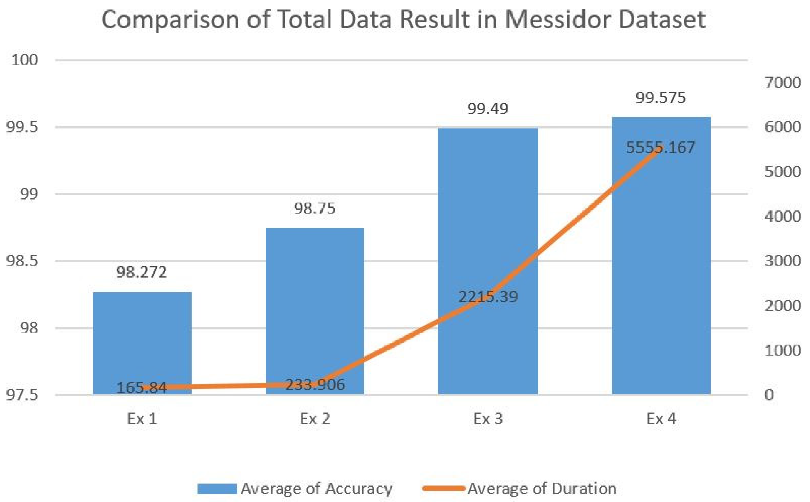
| Experiment | Number of Training Data | Number of Testing Data | Accuracy (%) | Sensitivity (%) | Specificity (%) | Duration (s) |
|---|---|---|---|---|---|---|
| Ex 1 | 16,000 | 4000 | 98.27 | 98.27 | 98.28 | 165.84 |
| Ex 2 | 32,000 | 8000 | 98.75 | 98.75 | 98.75 | 233.91 |
| Ex 3 | 40,000 | 10,000 | 99.49 | 99.49 | 99.49 | 2215.39 |
| Ex 4 | 48,000 | 12,000 | 99.58 | 99.58 | 99.58 | 5555.17 |
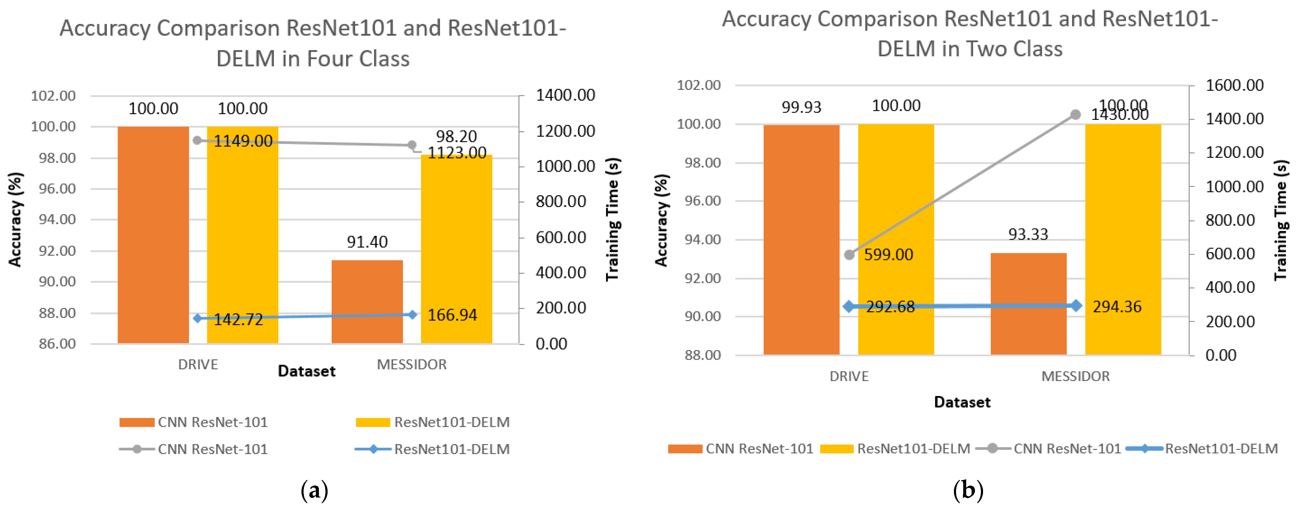
| 2 Class | ResNet-101 | ||||
| Dataset | Accuracy (%) | Sensitivity (%) | Specificity (%) | Duration (s) | |
| DRIVE | 99.93 | 99.93 | 99.93 | 599.00 | |
| MESIDOR | 92.99 | 92.99 | 93.05 | 594 | |
| ResNet-101-DELM | |||||
| DRIVE | 100.00 | 100.00 | 100.00 | 303.15 | |
| MESIDOR | 100.00 | 100.00 | 100.00 | 293.08 | |
| 4 Class | ResNet-101 | ||||
| Dataset | Accuracy (%) | Sensitivity (%) | Specificity (%) | Duration (s) | |
| DRIVE | 100.00 | 100.00 | 100.00 | 1149.00 | |
| MESIDOR | 91.40 | 91.40 | 91.49 | 1123.00 | |
| ResNet-101-DELM | |||||
| DRIVE | 100.00 | 100.00 | 100.00 | 142.72 | |
| MESIDOR | 98.20 | 98.20 | 98.19 | 166.94 | |
| Method | Dataset | Accuracy (%) | Sensitivity (%) | Specificity (%) | Duration (s) |
|---|---|---|---|---|---|
| 5-Layered CNN [46] | MESSIDOR | 98.15 | 98.94 | 97.87 | - |
| Modified Alexnet [12] | MESSIDOR | 92.35 | - | 97.45 | - |
| ResNet-101 [47] | DRIVE | 95.10 | 79.30 | 97.40 | - |
| CLAHE+ ResNet-101-DELM | DRIVE | 100.00 | 100.00 | 100.00 | 142.72 |
| CLAHE+ ResNet-101-DELM | MESIDOR | 98.20 | 98.20 | 98.19 | 166.94 |
Publisher’s Note: MDPI stays neutral with regard to jurisdictional claims in published maps and institutional affiliations. |
© 2022 by the authors. Licensee MDPI, Basel, Switzerland. This article is an open access article distributed under the terms and conditions of the Creative Commons Attribution (CC BY) license (https://creativecommons.org/licenses/by/4.0/).
Share and Cite
Novitasari, D.C.R.; Fatmawati, F.; Hendradi, R.; Rohayani, H.; Nariswari, R.; Arnita, A.; Hadi, M.I.; Saputra, R.A.; Primadewi, A. Image Fundus Classification System for Diabetic Retinopathy Stage Detection Using Hybrid CNN-DELM. Big Data Cogn. Comput. 2022, 6, 146. https://doi.org/10.3390/bdcc6040146
Novitasari DCR, Fatmawati F, Hendradi R, Rohayani H, Nariswari R, Arnita A, Hadi MI, Saputra RA, Primadewi A. Image Fundus Classification System for Diabetic Retinopathy Stage Detection Using Hybrid CNN-DELM. Big Data and Cognitive Computing. 2022; 6(4):146. https://doi.org/10.3390/bdcc6040146
Chicago/Turabian StyleNovitasari, Dian Candra Rini, Fatmawati Fatmawati, Rimuljo Hendradi, Hetty Rohayani, Rinda Nariswari, Arnita Arnita, Moch Irfan Hadi, Rizal Amegia Saputra, and Ardhin Primadewi. 2022. "Image Fundus Classification System for Diabetic Retinopathy Stage Detection Using Hybrid CNN-DELM" Big Data and Cognitive Computing 6, no. 4: 146. https://doi.org/10.3390/bdcc6040146
APA StyleNovitasari, D. C. R., Fatmawati, F., Hendradi, R., Rohayani, H., Nariswari, R., Arnita, A., Hadi, M. I., Saputra, R. A., & Primadewi, A. (2022). Image Fundus Classification System for Diabetic Retinopathy Stage Detection Using Hybrid CNN-DELM. Big Data and Cognitive Computing, 6(4), 146. https://doi.org/10.3390/bdcc6040146