Article

Moving Object Detection Based on a Combination of Kalman Filter and Median Filtering

1
Department of Mathematical Modeling, North Caucasus Federal University, 355017 Stavropol, Russia
2
Department of Modular Computing and Artificial Intelligence, North-Caucasus Center for Mathematical Research, 355017 Stavropol, Russia
*
Author to whom correspondence should be addressed.
Big Data Cogn. Comput. 2022, 6(4), 142; https://doi.org/10.3390/bdcc6040142
Submission received: 26 October 2022 / Revised: 9 November 2022 / Accepted: 22 November 2022 / Published: 25 November 2022

Abstract

:
The task of determining the distance from one object to another is one of the important tasks solved in robotics systems. Conventional algorithms rely on an iterative process of predicting distance estimates, which results in an increased computational burden. Algorithms used in robotic systems should require minimal time costs, as well as be resistant to the presence of noise. To solve these problems, the paper proposes an algorithm for Kalman combination filtering with a Goldschmidt divisor and a median filter. Software simulation showed an increase in the accuracy of predicting the estimate of the developed algorithm in comparison with the traditional filtering algorithm, as well as an increase in the speed of the algorithm. The results obtained can be effectively applied in various computer vision systems.

1. Introduction

At present, the solution of problems related to the determination of a moving object and the distance to it is practically significant in various robotic systems, including computer vision systems [1]. The distance to the object is determined in video monitoring systems for security [2], navigation [3], surveillance [4], control [5], etc. In turn, systems that solve the problem of detecting a moving object and determining the distance to it put forward increased technical and hardware requirements. Since, first of all, the process of detecting a moving object is complicated by the presence of projective, affine distortions, as well as distortions from receivers, the computational algorithms on which the systems are built should not only process the video sequence of data at real speed in real time, but also qualitatively process the data received from various types of distortions and artifacts. For this reason, there is a search, development of high-quality and new computational methods and algorithms used to solve the designated range of problems including in terms of quality while reducing the variability of the technological process [6].
Currently, solving problems related to determining the distance to an object is practically significant in various robotic systems, including computer vision systems [7]. Modern computer vision systems obtain real information about the distance to objects using various sets of sensors, such as radar [8], ultrasonic sensors [9], lidars [10], stereo mate [11], etc.
At the same time, in various applications (unmanned vehicles, mobile applications), the approach of merging lidar and camera sensors is becoming more widespread [12]. In [13], the authors propose an approach to merge several lidar sensors and a color camera in real time to recognize multi-scale objects at the semantic level, which makes it possible to adapt the developed module to complex scenes.
The procedure for the simultaneous use of such sensors is that the common sensor receives a combination of data coming from the camera in the form of an image, and from the lidar in the form of a cloud of points. After that, the resulting point cloud is projected onto the image. The position of the point cloud in the image is the determined distance to the moving object. In [14], the authors propose to determine the distance to objects of known sizes and geometry in order to improve the estimation of the position of the object before quantization and to obtain systematic errors inherent in lidar. The authors also propose in their work to apply the fitting method to convert the lidar into a monocular camera, which avoids the task of extracting the target edge from the point cloud. For successful sensor fusion, [15] used sparse and accurate point clouds as a guideline for determining the correspondence of stereo images in a single three-dimensional volume space. In [16], a lidar-camera fusion approach was developed to correct oscillating lidar distortions with full velocity estimation. A new mechanism for quantifying and analyzing 3D motion correlation for estimating real-time temporal displacement of fusion of dissimilar sensors is described by the authors of [17]. A multi-sensor platform for combining camera and lidar data for object detection, including small obstacles and moving objects, is proposed in [18]. A new merge pipeline based on the method of early fusion of image range and RGB image to improve the detection of 3D objects is proposed in [19]. A new approach to the use of a convolutional neural network that detects and identifies an object based on data obtained from a 3D lidar is described in [20]. Paper [21] presents a new method for estimating the transformation between the manipulator camera and the 2D lidar coordinate system, based on the use of point, line, and plane geometry constraints between the segmented 2D lidar scan and the reconstructed trihedron elements. The proposed spatiotemporal sampling algorithm activates the lidar only in areas of interest identified by analyzing visual input and reduces the base lidar frame rate according to the kinematic state of the system in [22]. In [23], the authors, before calibrating the lidar camera, use a new method in which they align 3D visual points on laser scans based on the tight coupling graph optimization method to calculate the external parameter between the lidar and the camera. The approach in [24] uses the geometric information provided by the point cloud as prior knowledge and clusters the point cloud data using an improved density clustering algorithm to further combine data from lidar and camera sensors. The authors of [25] at the theoretical level analyzed the limitations imposed by boundary objects and the sensitivity of the calibration accuracy to the distribution of boundaries in the scene, and at the implementation level, they proposed a method for detecting lidar boundaries based on cutting voxels from a point cloud and fitting the plane. Three different approaches for combining image characteristics with point cloud data in which lidar reflection data can be replaced with low-level image characteristics without degrading detector performance have been developed by researchers [26]. To solve the problem of combining data from different types of lidar and camera sensors, the authors of [20] developed a multimodal system for detecting and tracking 3D objects (EZFusion). The classification of 3D LiDAR point clouds using a visual object detector and an object tracker that jointly performs detection and tracking of 3D objects before data calibration is used in [27]. The authors of the study [28] solve the problem of segmentation of moving objects. The authors combine the steps of segmentation, background initialization, feature extraction, plotting, graph signal selection, and semi-supervised learning algorithm and explain the theoretical background, and propose two architectures for semi-supervised learning segmentation and a new evaluation procedure for GPS-based segmentation algorithms. One paper [29] proposed a processing method for practical applications under conditions of strong input uncertainty.
However, in all the listed works, the sensor data are calibrated without their preliminary processing. Since there may be impulsive noise among the data during projection, then in this case, in order to improve the accuracy of distance estimation, the received data require primary processing with a digital filter. From this point of view, a suitable tool is the median filter [30], which allows cleaning data from impulse noise. On the other hand, the process of combining several sensors at the same time requires the use of a suitable algorithm that allows you to work with multiple input signals. The Kalman filter [31] is a recursive filter capable of predicting the future state of a system based on previous data.
However, in real-time computer vision systems, the process of estimating the distance to a moving object should be as fast as possible. The presence of the division operation in the traditional Kalman filter algorithm increases the computational cost [32]. There are various approaches that allow to increase the speed of a computing system built on the basis of the Kalman filter, among which are [32,33,34] and others.
However, the existing real Kalman filtering methods for solving the problem of detecting a moving object use the traditional structure of the algorithm. Such a structure includes the execution of a division operation. This is a problematic application of this approach in terms of the computational delay of the algorithm and the quality of data processing in real time. In this paper, we propose an algorithm that includes combinational filtering of data based on a median filter used to filter a point cloud and a modified Kalman filter with a Goldschmidt divider used to predict estimates of distances to a moving object. The modified Kalman filter algorithm, including the Goldschmidt divider, replaces the division operation by reducing it to iterative multiplication, which allows to speed up data processing, thereby reducing computational costs. The median filter is used to preprocess data from impulse noise. The modified algorithm proposed by us, built on the basis of the integration of these solutions, made it possible to obtain advantages in the form of a reduction in the time delay and the error in calculating the distance to a moving object. Software simulation confirms the obtained results.
The article includes: Section 1 containing preliminary information and problem statement; Section 2, which introduces the developed filter algorithm; Section 3, which describes software and experimental simulations of filter accuracy and time performance estimates.

2. Materials and Methods

The Kalman filter is a recursive probabilistic filter. Based on the filter, the past state, present state and future state of the dynamic system are determined [35]. The entire filtering procedure is divided into two processes: performing prediction and updating the state. The predicted state is a mathematical model (1) and (2). They use previous and input data received from a series of sensors:
x ¯ k = A x k 1 + B u k 1
where x ¯ k —state variable vector, A —transition matrix between system states, B —control matrix and u k 1 —system control action at the previous moment of time.
P ¯ k = A P k 1 A T + Q
where P ¯ k —error covariance matrix and Q —technological noise covariance matrix.
The updated state uses the predicted state value to perform the next prediction step. The updated state is calculated using Equations (4) and (5):
K k = P ¯ k 1 H P ¯ k 1 H T + R
x ^ k = x ¯ k 1 + K k ( y k H x ¯ k 1 )
P ^ k = ( I K k H ) P ¯ k 1
where K k —Kalman gain, H —measurement matrix showing the relationship between measurements and the state of the system, R —measurement noise matrix, y k —measurement of the system state at the current time and I —identity matrix.
However, the step of updating the states of a dynamical system requires a preliminary determination of the value of the Kalman gain (3) [36]. Since Kalman gain involves performing a division operation, it can be concluded that gain calculation is the most computationally expensive operation.
There are many methods for designing fission equipment. Among which we can single out the quadratically convergent Goldschmidt algorithm [37]. A feature of this algorithm is the ability to obtain the result of division without a remainder. Then, this algorithm is defined by Equation (6):
N = a F i b F i
where coefficient F i = 2 b . In Section 2, we will show the application of the Goldschmidt algorithm in the Kalman filter when calculating the gain K k , and we will also use the median filter to filter the point cloud projected onto the input image.
The median filter is a non-linear digital filter [38]. Such a filter is used in image and signal processing to remove impulse noise and smooth the signal. In systems that receive information using sensors, the signals always have noise from the environment and noise from the loss of sensors.
The process of median filtering is to obtain the signal values in the form of a variational series built in ascending or descending order. Signal values are taken in the vicinity of some point (filter window). To solve the task of determining the distance to a moving object, the median filter will select a cloud of points from the input images using nearby data. Thus, if we designate the filtered selection of array elements as D = { d 1 ,   d 2 ,   ,   d n } , so that the number of selection elements coincides with the size of the filter window, then the application of median filtering, which selects the central values of the ordered selection, can be written as:
x = m e d ( d 1 ,   d 2 ,   ,   d n )

3. Results

This section presents a filtering algorithm that uses the median filtering method, as well as a modified Kalman filter based on the Goldschmidt divisor.

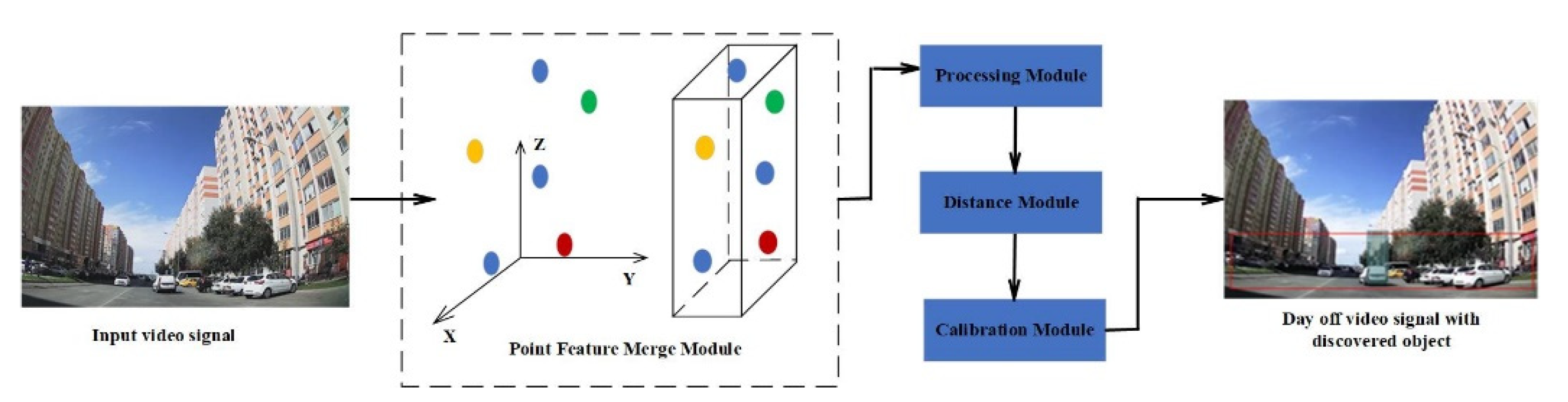
3.1. Proposed Algorithm

The proposed model of the process of determining the distance to a moving object based on the fusion of camera and lidar sensors is shown in Figure 1. The presented model uses a cloud of points obtained by lidar and an RGB image obtained from a video camera as input and predicts oriented 3D frames for moving objects (cars, pedestrians, cyclists).
This model includes four main modules: Point Merge Module, which extracts point features from an RGB image and combines the extracted features with the corresponding point cloud features, Value Calibration Module, Merged Values Processing Module and Object Distance Module. Below is a filtering algorithm that uses the median filtering method, as well as a modified Kalman filter, built on the basis of the Goldschmidt divider, used in the modules for processing and determining the distance.
The processing of lidar data can be represented in several stages. At the first stage, lidar points are captured, after which all points in a single system are complexed and reduced to a single coordinate system or a uniform grid. The grid is created by transforming between irregular raw lidar measurements and a grid at regular intervals. The m×n grid dimensions are defined as follows:
m = ( y m a x y m i n G s ) + 1
n = ( x m a x x m i n G s ) + 1
where m is the number of grid rows, n is the number of columns in the grid and G s is the grid cell size depending on the lidar data density. The denser the raw data, the smaller the cell size and vice versa. Thus, after appropriate transformations, all coordinates of the lidar measurement are assigned to each grid cell.
All data have a certain amount of noise, so the next step is to filter these data. Since an isolated outlier is a noise point that is isolated from the main point cloud, it remains to determine how far it is from the point cloud. At this stage, the algorithm proposed in the paper applies median data filtering. To do this, point clouds are divided into voxels of a given size and a minimum number of voxel points.
Voxels that do not pass the test are discarded, leaving only useful points that carry information about objects. This approach is effective for lidars with a large number of points and allows you to analyze the entire three-dimensional matrix of voxels, based on the occupancy of neighboring cells, passing through the filter through all points sequentially.
Let some point m = [ u ,   v ] T on the image plane be given. Moreover, it is a projection of some point M = [ X , Y , Z ] T in the space of the point cloud. Then the relationship between these points can be written as:
S m = W [   R t ] M
where S —some scalar, R and t —external parameters of the camera and W —matrix of internal parameters of the camera (10):
W = [ α γ x o 0 β y o 0 0 1 ]
where ( x 0 , y 0 ) —coordinates of the point, α and β —compression ratios along the Ox and Oy axes and γ —coefficient of asymmetry between the image axes. We take Z = 0 and denote by r i j the i-th element of the rotation matrix R . Then the projective matrix M p (10), which projects the point cloud onto the image obtained by calibrating the lidar and camera sensors, will take the form:
M p = [ r 11 r 12 x 0 r 21 r 22 y 0 0 0 1 ]
Then, we rewrite (10) for a point on the object M = [ X , Y , 1 ] T and the corresponding point on the image m in the form:
S m = L M
where L —image homography matrix, defined as:
L = W [ r 1 r 2 t ]
Let us find the homography matrix; for this, we introduce the covariance matrix Φ m i :
i ( m i m i ) T Φ m i 1 ( m i m i )
where m i is determined from Equation (15):
m i = 1 l ¯ 3 T M i [ l ¯ 1 T M i l ¯ 2 T M i ]
where l ¯ i —i-th row of the matrix L .
Let L = [ l 1 l 2 l 3 ] , then from (12) we obtain:
[ l 1 l 2 l 3 ] = λ W [ r 1 r 2 t ]
where λ —some scalar. Knowing that r 1 and r 2 are orthogonal, then we write:
l 1 T W T W 1 l 2 = 0
l 1 T W T W 1 l 1 = l 2 T W T W 1 l 2
For v i j , we obtain:
v i j = [ l i 1 l j 1 , l i 1 l j 2 + l i 2 l j 1 , l i 2 l j 2 + l i 3 l j 1 + l i 1 l j 3 , l i 3 l j 2 + l i 2 l j 3 , l i 3 l j 3 ] T
Then, we rewrite (18) and (19) as:
[ v 12 T ( v 11 v 22 ) T ] e = 0
where the vector e :
e = [ E 11 ,   E 12 ,   E 22 ,   E 13 ,   E 23 ,   E 33   ]
E i j matrix elements E = W T W 1 . Then, to determine the matrix W of the internal parameters of the camera, it suffices to use n images and Equation (19):
v 0 = ( E 12 E 13 E 11 E 23 ) / ( E 11 E 22 E 12 2 )
λ = E 33 [ E 13 2 + v 0 ( E 12 E 13 E 11 E 23 ) ] / E 11
α = λ / E 11
β = λ E 11 / ( E 11 E 22 E 12 2 )
γ = E 12 α 2 β λ
u 0 = c v 0 α E 13 α 2 λ
After determining the matrix W , it is possible to determine the homography matrix, and using expression (11) to carry out a complete projection of the point cloud into the image space. Denote d i j = L M . Then, after projecting the points, we obtain some matrix of values:
D = [ d 11 d 1 j d i 1 d i j ]
We will apply a median filter with a weighted weight vector V of size N to the resulting array of values for pre-processing and removal of impulse noise. Data processing is as follows. We have an input sequence such as D = { d 1 ,   d 2 ,   ,   d n } . Then, after some algebraic transformations using replication over each value of the vector V, the median filtering output is calculated as:
x ( n ) = m e d i a n ( V 1 d 1 , V 2 d 2 ,   , V n d n )
where V n are the values of the weight vector and is the replication operator. In what follows, we will use a median filtering window of size N = 5 . In this case, we obtain a symmetric weight vector V = [ V 1 , V 2 , V 3 , V 2 , V 1 ] and an observation   D = [ d 1 , d 2 , d 3 , d 4 , d 5 ] . Then, from (21), the filter output will be as follows:
x ( n ) = m e d i a n [ V 1 d 1 , V 2 d 2 , V 3 d 3 , V 4 d 4 , V 5 d 5 ] = m e d i a n [ d 1 , d 2 , d 2 , d 3 , d 3 , d 3 , d 4 , d 4 , d 5 ] = m e d i a n [ d 4 , d 4 , d 3 , d 3 , d 3 , d 2 , d 2 , d 5 , d 1 ] = d 3
The approach associated with the use of median filtering will improve the accuracy of the position of the point cloud to further determine the distance to the object. After receiving the processed data, a digital Kalman filter is applied to them. The Kalman filter can predict future status based on previous data. We propose a modified Kalman filter algorithm based on the use of the Goldschmidt divider to calculate the Kalman gain value.
Thus, based on the conditions described, the paper proposes an algorithm for implementing data filtering to detect the distance to an object in a video data stream (Algorithm 1).
Algorithm 1: Data filtering using median filter and Kalman filter built using the Goldschmidt algorithm to calculate the Kalman gain
Input data:
1:        { m ,   M , S ,   R ,   L , E , r 1 , r 2 , t ,   x 0 , i , P o , i , A ,   B ,   C , D ,   H , Q , R }
Calibration of sensor values:
Determination of the internal parameters of the camera matrix W :
2.         v 0 = ( E 12 E 13 E 11 E 23 ) / ( E 11 E 22 E 12 2 )
3.           λ = E 33 [ E 13 2 + v 0 ( E 12 E 13 E 11 E 23 ) ] / E 11
4.               α = λ / E 11
5.            β = λ E 11 / ( E 11 E 22 E 12 2 )
6.             γ = E 12 α 2 β λ
7.           u 0 = c v 0 α E 13 α 2 λ
Definition of homography matrix:
8.           L = W [ r 1 r 2 t ]
Projection matrix calculation   D :
9.             d i j = L M
Calculation of median filtering values:
10.             x = m e d i a n ( d 1 , d 2 , , d n )
gKalman filtering:
Prediction Calculation:
11:            x ¯ k = A x k 1 + B u k 1
12:                P ¯ k = A P k 1 A T + Q
Kalman gain calculation:
13:                b 0 = H P ¯ k H T + R
14:                 F k = 2 b k
15.                N k = N k 1 F k
16:                b k = b k 1 F k
If b k = 1 , then
17:                K k = P ¯ k H T b k
other F k + 1 = 2 b k ,
Update Calculation:
18:             x ^ k = x ¯ k 1 + K k ( y k H x ¯ k 1 )
19:                P ^ k = ( I K k H ) P ¯ k 1
The developed algorithm makes it possible to obtain such a filter design that is capable of processing data obtained after calibrating the values coming from different types of sensors. At the same time, the use of median filtering preliminarily clears the projected data from different planes from impulse noise. In turn, the modified Kalman filter, due to the use of the Goldschmidt algorithm in calculating the Kalman gain, makes it possible to avoid the division operation in the filter design, which will reduce computational costs during filtering.
Let us consider the numerical implementation of the algorithm described above, which proves the effectiveness of the proposed algorithm and theoretical results in comparison with the known algorithm.

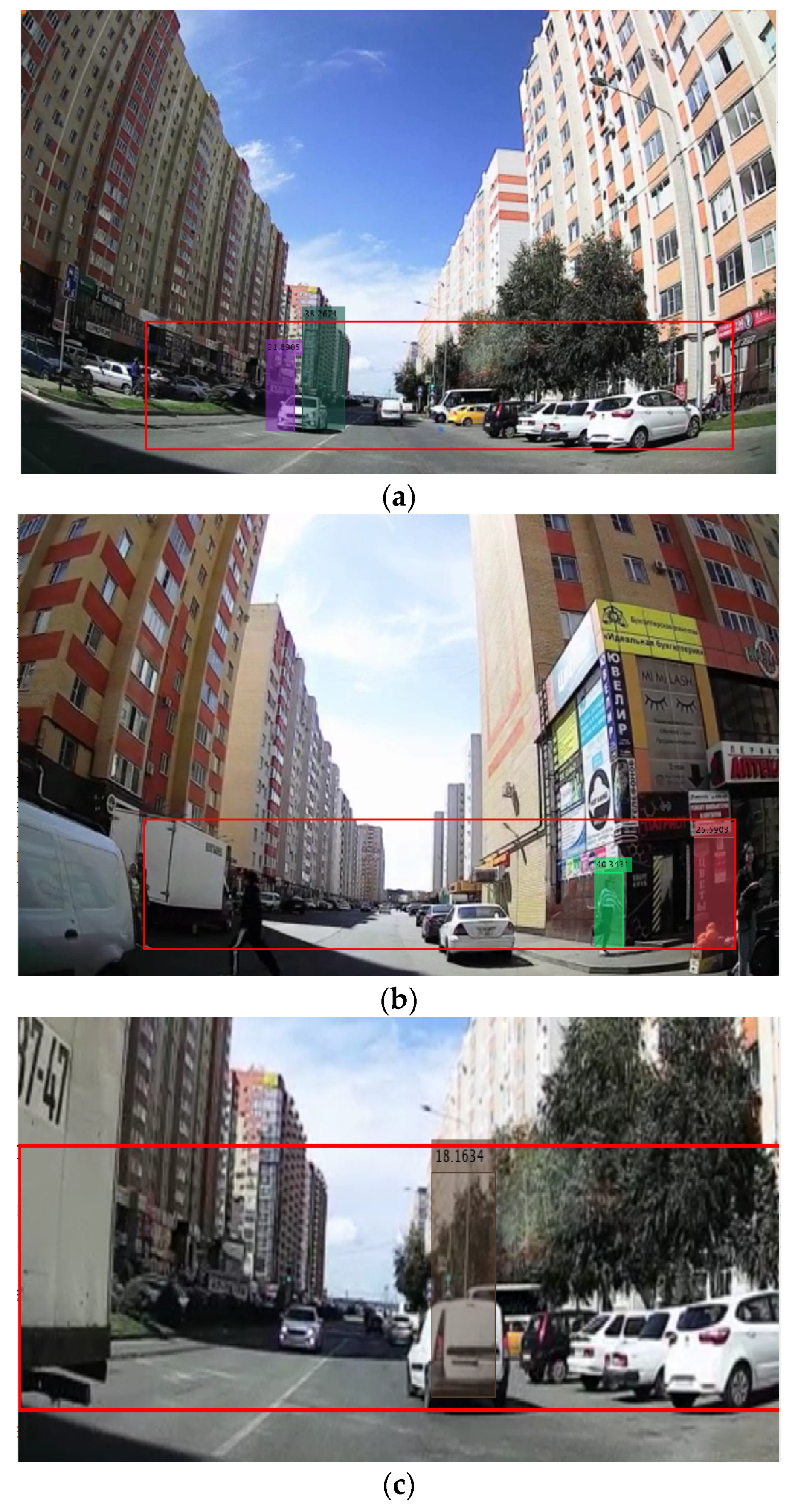
3.2. Numerical and Software Implementation

Let the system under consideration consist of two sensors: a lidar sensor and a camera from which images are received. The system matrices and input data are proposed to be equal: m = [ 4 ,   3 ] T , M = [ 2 , 1 , 0 ] T , W i = 10 × 10 ;   α = β = 1 , γ = 0 , R = 1 , t = 1 , Δ T = 0.05 —sampling time for each frame, B = 0 , τ = 0.05 —measurement noise variance.
A = [ 1 0 Δ T 0 0 1 0 Δ T 0 0 1 0 0 0 0 1 ]
Q = [ Δ T 4 / 4 0 Δ T 3 / 2 0 0 Δ T 4 / 4 0 Δ T 3 / 2 Δ T 3 / 2 0 Δ T 2 0 0 Δ T 3 / 2 0 Δ T 2 ] τ 2
R = [ τ 1 0 0 0 0 τ 1 0 0 0 0 τ 1 0 0 0 0 τ 1 ]
H = [ 1 0 0 0 0 1 0 0 1 0 0 0 0 1 0 0 ]
A comparison of the simulation results for the well-known Kalman filtering algorithm and the developed algorithm is presented in Table 1. The error in determining the distance was found as the difference between the true value of the distance and the determined one. Each scenario number has a different distance. Simulation was carried out on 10 scenarios with different true distance values, respectively, from 1 to 10 m.
To assess the influence of key parameters affecting performance in the known algorithms [31, 35] and the proposed algorithm, we will carry out their numerical simulation to solve the problem of determining the state of a dynamic system at the next time point for 100 consecutive measurements. As input data, we will use the following system matrices and input data that will describe the position of the object and update this estimate:
A k = ( 0.3 × ( 1 + 0.01 t k ) 0.01 0.1 0.96 ) , B k = I ,   Q k = 0.1 × I ,
R = ( 0.02 0.06 0.07 0.07 ) ,       H = ( 1 0 )
The time sequence { t k } lies in the interval [0, 10] with a uniform sampling step of 0.1; therefore, k = 0 , 1 , , 100 . Initial filter setting: x ^ 1 , 0 = 1 and P 1 , 0 = 100 × I . The performance check and accuracy of all three algorithms will be evaluated using different input values of the matrix P 0 . This matrix is the state covariance matrix and affects the confidence of the filter in estimating the state variables. We will evaluate the accuracy of the algorithm by calculating the root mean square error (RMSE) for each specific state of the system:
R M S E = i = 1 n ( E r r o r i ) 2 n 1
The simulation results are presented in Table 2. The obtained results show that the calculation error, which depends on the measurement noise in the developed method, decreases by 0.7 and 0.6 in comparison with the [35, 31] algorithms. The application of the Goldschmidt algorithm in the structure of the developed filter makes it possible to reduce the computational delay by 2.9 and 2.4 times, respectively. At the same time, the variation of the parameter of the covariance matrix shows that they practically do not affect the time delay of the filter; however, an increase in the values of the matrix leads to an increase in the mean square error of the filter for all three algorithms.
Figure 2 shows the results of software simulation. To carry out software simulation, archival data were used in the form of a video file with a frame size of 720 × 1280 and an input rate of up to 30 frames per second. The simulation was carried out using the Matlab R2021a software package. The purpose of the simulation is to measure the distance from the sensor to the object. A moving object is determined by analyzing a sequence of points for four situations. This takes into account that the sequence of points is interrupted only when no re-reflection has occurred. If this did not happen, then we are dealing with an object that strongly refracts waves. Thus, the sequence of points can be refracted with a shift closer to the vehicle. Thus, we are dealing with a convex obstacle; in this case, by a convex obstacle, we mean cars, people, etc. By the magnitude of the shift, we can judge the size of the obstacle. If the sequence of points is not interrupted, we obtain a solid line, and there are no obstacles. When a sequence of points is refracted with a shift from the vehicle, then we are dealing with a concave obstacle (puddle, pit, etc.). Having determined all the obstacles, the algorithm determines the contours of the moving object from all sides.
Thus, the object of interest is within the bounding box, where the box is created by detecting the object. The determined distance corresponds to the measured distance from the point cloud. The data are unstable due to the large number of point clouds from the environment and objects in the bounding box. There was a difficulty in choosing an objective point cloud. The median filter helps select a bounding box point cloud using nearby data. The domain code is in the public domain [39].

4. Discussion

The obtained results show that the developed algorithm gives a gain in the measurement error due to the use of the median filter and the detection time of the distance to the object in the video data stream. Moreover, the greater the distance to the object, the higher the error and the time of determining the distance.
As a result of the program, the distance to moving objects is determined. During the entire video sequence, moving objects can be covered by other objects, and projective transformations associated with camera tilt do not occur. However, there are affine transformations associated with scalability and rotation of moving objects. The results obtained make it possible to determine the distance to moving objects when this object is overlapped in computer vision systems.

5. Conclusions

In this paper, we studied the solution of the problem of determining the distance to an object using the well-known Kalman filtering algorithm and the developed filtering algorithm, which uses the Goldschmidt divider design to improve the performance of the computing system. Additionally, the developed algorithm includes a block of median data filtering to improve the accuracy of determining the distance to the object. The results of software simulation showed a faster determination of the distance to an object in the video data stream, as well as a smaller error in such determination. The results obtained showed that the developed algorithm can be applied in computer vision systems to combine data obtained from different types of sensors. In addition, the proposed algorithm should be applied in computer vision systems, where a critical indicator is to increase the performance of the system, i.e., indicator of the time delay of the system.
Further research will be aimed at developing the hardware implementation of the developed algorithm, the architectural implementation of the median filtering units, and the modified algorithm divider, as well as comparing the work of the developed architectures in positional and non-positional number systems.

Author Contributions

Conceptualization, D.K. and P.L.; methodology, P.L.; software, D.K.; validation, D.K.; formal analysis, P.L.; investigation, D.K.; resources, P.L.; data curation, D.K.; writing—original draft preparation, D.K.; writing—review and editing, P.L.; visualization, D.K.; supervision, P.L.; project administration, P.L.; funding acquisition, D.K. and P.L. All authors have read and agreed to the published version of the manuscript.

Funding

The work was supported by the Council for Grants of the President of the Russian Federation under Project MK-3918.2021.1.6.

Institutional Review Board Statement

Not applicable.

Informed Consent Statement

Not applicable.

Data Availability Statement

Not applicable.

Acknowledgments

The authors would like to thank North-Caucasus Federal University for supporting in the contest of projects competition of scientific groups and individual scientists of North-Caucasus Federal University.

Conflicts of Interest

The authors declare no conflict of interest. The funders had no role in the design of the study; in the collection, analyses or interpretation of data; in the writing of the manuscript; or in the decision to publish the results.

References

  1. Wong, C.-C.; Chien, M.-Y.; Chen, R.-J.; Aoyama, H.; Wong, K.-Y. Moving Object Prediction and Grasping System of Robot Manipulator. IEEE Access 2022, 10, 20159–20172. [Google Scholar] [CrossRef]
  2. Singha, A.; Bhowmik, M.K. Salient Features for Moving Object Detection in Adverse Weather Conditions During Night Time. IEEE Trans. Circuits Syst. Video Technol. 2020, 30, 3317–3331. [Google Scholar] [CrossRef]
  3. Shi, W.; Shan, R.; Okada, Y. A Navigation System for Visual Impaired People Based on Object Detection. In Proceedings of the 2022 12th International Congress on Advanced Applied Informatics (IIAI-AAI), Kanazawa, Japan, 2–8 July 2022; pp. 354–358. [Google Scholar]
  4. Baiju, P.S.; George, S.N. An Automated Unified Framework for Video Deraining and Simultaneous Moving Object Detection in Surveillance Environments. IEEE Access 2020, 8, 128961–128972. [Google Scholar] [CrossRef]
  5. Sultana, M.; Mahmood, A.; Jung, S.K. Unsupervised Moving Object Detection in Complex Scenes Using Adversarial Regularizations. IEEE Trans. Multimedia 2021, 23, 2005–2018. [Google Scholar] [CrossRef]
  6. Grishaeva, S.A.; Barmenkov, E.Y.; Borisova, E.V. Features of Advanced Product Quality Planning in the Space Industry Enterprises. In Proceedings of the 2021 International Conference on Quality Management, Transport and Information Security, Information Technologies (IT&QM&IS), Yaroslavl, Russia, 6–10 September 2021; pp. 293–297. [Google Scholar]
  7. Rahmadya, B.; Sun, R.; Takeda, S.; Kagoshima, K.; Umehira, M. A Framework to Determine Secure Distances for Either Drones or Robots Based Inventory Management Systems. IEEE Access 2020, 8, 170153–170161. [Google Scholar] [CrossRef]
  8. Lee, T.-Y.; Skvortsov, V.; Kim, M.-S.; Han, S.-H.; Ka, M.-H. Application of Band FMCW Radar for Road Curvature Estimation in Poor Visibility Conditions. IEEE Sens. J. 2018, 18, 5300–5312. [Google Scholar] [CrossRef]
  9. Wang, L.; Wang, T.; Liu, H.; Hu, L.; Han, Z.; Liu, W.; Guo, N.; Qi, Y.; Xu, Y. An Automated Calibration Method of Ultrasonic Probe Based on Coherent Point Drift Algorithm. IEEE Access 2018, 6, 8657–8665. [Google Scholar] [CrossRef]
  10. Balemans, N.; Hellinckx, P.; Steckel, J. Predicting LiDAR Data from Sonar Images. IEEE Access 2021, 9, 57897–57906. [Google Scholar] [CrossRef]
  11. Toth, M.; Stojcsics, D.; Domozi, Z.; Lovas, I. Stereo Odometry Based Realtime 3D Reconstruction. In Proceedings of the 2018 IEEE 16th International Symposium on Intelligent Systems and Informatics (SISY), Subotica, Serbia, 13–15 September 2018; pp. 000321–000326. [Google Scholar]
  12. Deng, Q.; Li, X.; Ni, P.; Li, H.; Zheng, Z. Enet-CRF-Lidar: Lidar and Camera Fusion for Multi-Scale Object Recognition. IEEE Access 2019, 7, 174335–174344. [Google Scholar] [CrossRef]
  13. Huang, J.-K.; Grizzle, J.W. Improvements to Target-Based 3D LiDAR to Camera Calibration. IEEE Access 2020, 8, 134101–134110. [Google Scholar] [CrossRef]
  14. Choe, J.; Joo, K.; Imtiaz, T.; Kweon, I.S. Volumetric Propagation Network: Stereo-LiDAR Fusion for Long-Range Depth Estimation. IEEE Robot Autom. Lett. 2021, 6, 4672–4679. [Google Scholar] [CrossRef]
  15. Yang, W.; Gong, Z.; Huang, B.; Hong, X. Lidar With Velocity: Correcting Moving Objects Point Cloud Distortion from Oscillating Scanning Lidars by Fusion with Camera. IEEE Robot Autom. Lett. 2022, 7, 8241–8248. [Google Scholar] [CrossRef]
  16. Qiu, K.; Qin, T.; Pan, J.; Liu, S.; Shen, S. Real-Time Temporal and Rotational Calibration of Heterogeneous Sensors Using Motion Correlation Analysis. IEEE Trans. Robot. 2021, 37, 587–602. [Google Scholar] [CrossRef]
  17. Zhangyu, W.; Guizhen, Y.; Xinkai, W.; Haoran, L.; Da, L. A Camera and LiDAR Data Fusion Method for Railway Object Detection. IEEE Sens. J. 2021, 21, 13442–13454. [Google Scholar] [CrossRef]
  18. Zhang, Z.; Liang, Z.; Zhang, M.; Zhao, X.; Li, H.; Yang, M.; Tan, W.; Pu, S. RangeLVDet: Boosting 3D Object Detection in LIDAR with Range Image and RGB Image. IEEE Sens. J. 2022, 22, 1391–1403. [Google Scholar] [CrossRef]
  19. Zhao, X.; Sun, P.; Xu, Z.; Min, H.; Yu, H. Fusion of 3D LIDAR and Camera Data for Object Detection in Autonomous Vehicle Applications. IEEE Sens. J. 2020, 20, 4901–4913. [Google Scholar] [CrossRef] [Green Version]
  20. Liu, C.; Huang, Y.; Rong, Y.; Li, G.; Meng, J.; Xie, Y.; Zhang, X. A Novel Extrinsic Calibration Method of Mobile Manipulator Camera and 2D-LiDAR via Arbitrary Trihedron-Based Reconstruction. IEEE Sens. J. 2021, 21, 24672–24682. [Google Scholar] [CrossRef]
  21. Ma, L.; Li, Y.; Li, J.; Tan, W.; Yu, Y.; Chapman, M.A. Multi-Scale Point-Wise Convolutional Neural Networks for 3D Object Segmentation from Lidar Point Clouds in Large-Scale Environments. IEEE Trans. Intell. Transp. Syst. 2021, 22, 821–836. [Google Scholar] [CrossRef]
  22. Fu, B.; Wang, Y.; Ding, X.; Jiao, Y.; Tang, L.; Xiong, R. LiDAR-Camera Calibration Under Arbitrary Configurations: Observability and Methods. IEEE Trans. Instrum. Meas. 2020, 69, 3089–3102. [Google Scholar] [CrossRef] [Green Version]
  23. Cui, M.; Zhu, Y.; Liu, Y.; Liu, Y.; Chen, G.; Huang, K. Dense Depth-Map Estimation Based on Fusion of Event Camera and Sparse LiDAR. IEEE Trans. Instrum. Meas. 2022, 71, 7500111. [Google Scholar] [CrossRef]
  24. Yuan, C.; Liu, X.; Hong, X.; Zhang, F. Pixel-Level Extrinsic Self Calibration of High Resolution LiDAR and Camera in Targetless Environments. IEEE Robot Autom. Lett. 2021, 6, 7517–7524. [Google Scholar] [CrossRef]
  25. Csontho, M.; Rovid, A.; Szalay, Z. Significance of Image Features in Camera-LiDAR Based Object Detection. IEEE Access 2022, 10, 61034–61045. [Google Scholar] [CrossRef]
  26. Li, Y.; Deng, J.; Zhang, Y.; Ji, J.; Li, H.; Zhang, Y. A Close Look at the Integration of LiDAR, Millimeter-Wave Radar, and Camera for Accurate 3D Object Detection and Tracking. IEEE Robot Autom. Lett. 2022, 7, 11182–11189. [Google Scholar] [CrossRef]
  27. Sualeh, M.; Kim, G.-W. Visual-LiDAR Based 3D Object Detection and Tracking for Embedded Systems. IEEE Access 2020, 8, 156285–156298. [Google Scholar] [CrossRef]
  28. Giraldo, J.H.; Javed, S.; Sultana, M.; Jung, S.K.; Bouwmans, T. The Emerging Field of Graph Signal Processing for Moving Object Segmentation. In International Workshop on Frontiers of Computer Vision; Springer: Cham, Switzerland, 2021; pp. 31–45. [Google Scholar]
  29. Zhang, W.; Li, X.; Ma, H.; Luo, Z.; Li, X. Universal Domain Adaptation in Fault Diagnostics with Hybrid Weighted Deep Adversarial Learning. IEEE Trans. Industr. Inform. 2021, 17, 7957–7967. [Google Scholar] [CrossRef]
  30. Thanh, D.N.H.; Hieu, L.M.; Enginoglu, S. An Iterative Mean Filter for Image Denoising. IEEE Access 2019, 7, 167847–167859. [Google Scholar] [CrossRef]
  31. Liu, H.; Hu, F.; Su, J.; Wei, X.; Qin, R. Comparisons on Kalman-Filter-Based Dynamic State Estimation Algorithms of Power Systems. IEEE Access 2020, 8, 51035–51043. [Google Scholar] [CrossRef]
  32. Pereira, P.T.L.; Paim, G.; da Costa, P.U.L.; da Costa, E.A.C.; de Almeida, S.J.M.; Bampi, S. Architectural Exploration for Energy-Efficient Fixed-Point Kalman Filter VLSI Design. IEEE Trans. Very Large Scale Integr. VLSI Syst. 2021, 29, 1402–1415. [Google Scholar] [CrossRef]
  33. Zhang, H.; Zhou, X.; Wang, Z.; Yan, H. Maneuvering Target Tracking with Event-Based Mixture Kalman Filter in Mobile Sensor Networks. IEEE Trans. Cybern. 2020, 50, 4346–4357. [Google Scholar] [CrossRef]
  34. Onat, A. A Novel and Computationally Efficient Joint Unscented Kalman Filtering Scheme for Parameter Estimation of a Class of Nonlinear Systems. IEEE Access 2019, 7, 31634–31655. [Google Scholar] [CrossRef]
  35. Peyman, S.; Saeid, H.; Simon, H. Kalman Filter. In Nonlinear Filters; Wiley: Hoboken, NJ, USA, 2022; pp. 49–70. [Google Scholar]
  36. Sayed, A.H. Kalman Filter. In Adaptive Filters; John Wiley & Sons, Inc.: Hoboken, NJ, USA; pp. 104–110.
  37. Piso, D.; Bruguera, J.D. Variable Latency Goldschmidt Algorithm Based on a New Rounding Method and a Remainder Estimate. IEEE Trans. Comput. 2011, 60, 1535–1546. [Google Scholar] [CrossRef]
  38. Green, O. Efficient Scalable Median Filtering Using Histogram-Based Operations. IEEE Trans. Image Process. 2018, 27, 2217–2228. [Google Scholar] [CrossRef] [PubMed]
  39. Lidar Kalman Filter Median. Available online: https://github.com/KalitaDiana/Lidar_Kalman_filter_median/blob/main/Lidar_Kalman_filter.m (accessed on 20 October 2022).
Figure 1. Model of the process of determining the distance to a moving object in a video data stream.
Bdcc 06 00142 g001
Figure 2. The result of software simulation of determining the distance from the object to the car. (a) The distance to the approaching object; (b) distance to turning objects; (c) distance to the receding object.
Bdcc 06 00142 g002
Table 1. Results in the measurement error and the time of determining the distance to the object in the known and proposed algorithm.
NoKnown AlgorithmAlgorithm 1
ErrorTemporary
Delay
ErrorTemporary
Delay
10.890.170.480.12
20.650.170.570.14
30.870.160.320.14
40.350.180.130.16
50.780.190.070.15
60.260.230.180.19
70.370.220.330.19
80.580.270.310.22
90.820.250.550.25
100.820.250.390.22
Table 2. Time delays and measurement errors of known Kalman filtering algorithms and the developed algorithm based on the Goldschmidt divider.
IndicatorAlgorithm
[35][31]Algorithm 1
DelayRMSEDelayRMSEDelayRMSE
P 0 1.08330.98710.90610.87220.37340.2135
100 P 0 1.08791.11090.90700.99690.38390.3368
500 P 0 1.08781.17700.90641.06220.38410.4021
Publisher’s Note: MDPI stays neutral with regard to jurisdictional claims in published maps and institutional affiliations.

