Abstract
Flying ad hoc networks (FANETs) or drone technologies have attracted great focus recently because of their crucial implementations. Hence, diverse research has been performed on establishing FANET implementations in disparate disciplines. Indeed, civil airspaces have progressively embraced FANET technology in their systems. Nevertheless, the FANETs’ distinct characteristics can be tuned and reinforced for evolving security threats (STs), specifically for intrusion detection (ID). In this study, we introduce a deep learning approach to detect botnet threats in FANET. The proposed approach uses a hybrid shark and bear smell optimization algorithm (HSBSOA) to extract the essential features. This hybrid algorithm allows for searching different feature solutions within the search space regions to guarantee a superior solution. Then, a dilated convolutional autoencoder classifier is used to detect and classify the security threats. Some of the most common botnet attacks use the N-BaIoT dataset, which automatically learns features from raw data to capture a malicious file. The proposed framework is named the hybrid shark and bear smell optimized dilated convolutional autoencoder (HSBSOpt_DCA). The experiments show that the proposed approach outperforms existing models such as CNN-SSDI, BI-LSTM, ODNN, and RPCO-BCNN. The proposed HSBSOpt_DCA can achieve improvements of 97% accuracy, 89% precision, 98% recall, and 98% F1-score as compared with those existing models.
1. Introduction
In recent years, unmanned aerial vehicles (UAVs) have attracted additional focus. The use of UAVs provides several distinct benefits over standard human-crewed airplanes, particularly concerning the operative charge, the operator’s protection, the UAVs’ functionality in arduous or risky settings, and their availability for civil implementations [1]. The latest technological developments have made it easy to set up an unmanned aerial system with a complex topology for crucial operations [2]. Their swift development and intense involvement in intelligent transportation (IT) has significantly affected the path that drone societies have attempted to establish for the prospective UAV systems. The present decentralized technology advances allow for diverse operations and the correlation of resources [3]. This technique permits unnecessary the use of crucial elements and enhances the system’s comprehensive strength [4]. Nevertheless, many contemporary developments in the network-attached UAV fleet domain concentrate on the path to attaining a drone network (DN) [5]. Low regard is given to the DN systems’ cyber security, resulting in the very advanced DN systems being defenseless against diverse STs [6,7].
This assures the data’s secrecy, attainability, and unity while transmitting during UAV-to-UAV transmission, and the safety of UAV-to-ground-node transmission remains a major problem experienced by FANETs. In FANETs, UAVs transfer data that encompass audio, video, image, text, GPS position, and other formats. In transmitting these data, they must possess a fine QoS, having low delay and error rates [8]. For dependable data delivery, FANETs send the most significant data in disparate deployments that must be dispatched in a time-bound way. Hence, the networks’ dependability remains excellent [9].
The compromised FANET-IoT devices (IoTD) in no way exhibit signs of being hacked and function as zombies for the botmaster (BM) when initiating the attacks [10]. A BN’s dimensions may remain small, comprising hundreds of bots, while a bigger BN can have thousands of bots. A few bots will be present on the dark web very inexpensively, while enormous BNs have heavy costs [11].
There are two kinds of BNs: (i) BNs accepting commands and in consistent interaction with the BM within a client–server framework; (ii) peer-to-peer bots that communicate independently with one another and initiate the attacks after obtaining the BM’s commands. BMs interact with bots by employing the aid of a command-and-control (CnC) server; the bots remain concealed until the BM gives commands. The concealed bots’ conduct creates infested bots and a botnet attack (BA), which is an intricate job [12]. The BAs include the following: (i) scan commands employed in discovering the defenseless IoTD; (ii) ACK, SYN, UDP, and TCP flooding; (iii) combination attacks employed in starting a link and transferring the spam into this [13]. The current drawback in UAV-assisted FANETs is the effective detection of security threats. For that purpose, the feature selection and classification methods need improvement. The contributions of this study are described below:
- A new technique is proposed that utilizes the hybrid shark and bear smell optimization algorithm (HSBSOA) for FS and the deep neural classifiers to enhance the efficient and precise BN identification approach in FANETs;
- The aim of this study remains in identifying and classifying the implementation-specified threats, such as scan attacks, DDoS, TCP, UDP, and sync flooding, which are a few of the typical attacks.
The proposed hybrid HSBSOpt_DCA approach allows for more precise multiclass classification, including various types of attacks and non-attacks (NAs), and has shown encouraging results. The organization of remainder of this paper is as follows. Section 2 provides a state-of-the-art literature review. Section 3, the Materials and Methods, discusses the dataset used and the proposed methods. Section 4 provides a detailed analysis and the results. Section 5 concludes the article.
2. Related Works
In [14], Fried and Last proposed a novel and optimistic technique of employing wide-range and publicly accessible flight records for training in machine learning (ML) paradigms, which could identify anomalous flight designs and was proven to be a coherent counteractant for many ADS-B attacks. This novel technique varies from the formerly proffered methodologies, incorporating elementariness with the present ADS-B system. In [15], Mall et al. discussed unsupervised settings with sensors fixed in specific regions where the data can be gathered via mobile gadgets that remain attached to a UAV or drone. The authors initially modeled an appropriate framework and a lightweight convention for initiating safe transmission amongst the gadgets and the cloud through a portable drone. This convention also employs the physically unclonable function’s (PUF) advantages for creation, which is employed to encrypt the messages in transmission. The familiar Scyther simulator is employed to stimulate the convention, and the outcomes show that this convention remains fully secured, preventing confidential data seepage.
In [16], Mairaj et al. attempted to learn the benefits of game-theoretic (GT) implementations for the avoidance of DDoSAs upon a drone emanating data out of standard game solutions, and optimized this with an encompassed authenticity concept named the quantal response equilibrium (QRE). The authors detected possible schemes for every player via simulations and devised five non-collaborative game scenarios for the DDoSAs’ two versions. In such games, the conventional GT resolution or Nash equilibrium (NashE) gives data regarding the drone’s suggested modes, the hacker’s favored scheme, and the GT threshold (TH), presuming that the participants remain exceptionally brilliant.
In [17], Popoola et al. suggested the federated DL (FDL) methodology for zero-day BA identification to prevent data secrecy seepage in IoT-edge gadgets (IoTEG). This study utilizes an optimal deep neural network (ODNN) framework for NT classification. A model parameter server (MPS) distantly organizes the DNN paradigms’ training in several IoTEGs when the federated averaging algorithm is employed to sum up the local paradigm updates. A global DNN paradigm is generated after many transmission rounds between the MPS and the IoTEG.
In [18], Hatzivasilis et al. introduced WARDOG, an awareness and digital forensic system, which notifies the end-user of the BN’s contamination, reveals the BN framework, and catches confirmable data, which is then employed in a law court. The accountable administration system collects the data and automatically creates documentation for each instance. The document comprises authentic forensic data tracing entire engaged bodies and their parts in the attack.
In [19], Xi et al. proposed convolutional neural networks (CNNs) with a new deep learning framework that consists of dilated convolutional neural networks and recurrent neural networks. These stacked dilated convolutional networks perform effective feature selection, and the softmax classifier is used to recognize activities, which increases the accuracy of the classification performance. In [20], Alharbi and Alsubhi proposed a graph-based machine learning (ML) technique for botnet detection. For feature evaluation, filter-based theories are used, which exhibit robustness to zero-day attacks. This method achieved high precision, but its accuracy was moderate. In [21], Sung et al. presented a new methodology for discovering the malware in GCSs, which employed a fastText paradigm to generate low-size vectors when compared with the vectors from one-hot encoding (OhE) and a bidirectional LSTM paradigm for a comparison alongside sequential opcodes (SO). Furthermore, the API function names were employed to enhance the classification precision of the SO. In the experimentation, the Microsoft malware classification competency database was employed, and the family types classified the malware within the database. This proffered methodology exhibited an execution enhancement of 1.8%, correlating with the execution of the OhE-related technique.
In [22], Shitharth and Prasad proposed the supervisory control and data acquisition (SCADA) systems with the Markov chain clustering (MCC) technique, rapid probabilistic correlated optimization (RPCO) approach, and block-correlated neural network (BCNN) method to improve the accuracy of the network. However, it failed to reduce the cost-effectiveness of the process. Several studies have executed intrusion and malware identification processes. Nevertheless, there is a deficit of research discussing the problems concerning BN detection and feature extraction, magnitude reductions to repress counterfeit data, overfitting, and meticulous criteria calibration. Many research studies have employed actual BA databases in actual settings.
Furthermore, studies have analyzed ML paradigms for synthetic BN data devoid of apportions for feature engineering and an exhaustive overfitting analysis. Many studies have employed unbalanced live databases for learning and BN identification. The research studies chiefly concentrate on achieving greater precision, without discussing the constraints of greatly unbalanced databases or acquiring ostensive precision. In Table 1, a summary is provided with the limitations of the earlier research studies.

Table 1.
Summary and limitations of some existing studies.
3. Proposed HSBSOpt_DCA
UAV sets can be linked with one another to function as a relay to transfer the data out of a remote area (RA) network. Generally, the UAVs possess a mission for a surveillance operation and an operation to create a relay network for gathering data from RAs, such as in a desert or jungle. The UAVs’ motility and versatility make it effortless to arrive at these RAs and give connectivity to the network. Nevertheless, with minor exertion, the attacker could effortlessly hijack the system. As a result, the deficit of a firm framework and the vulnerable wireless medium within FANETs make the nodes liable to attackers.
The N-BaIoT database comprises traffic data for pre-processing using the one-hot encoding method. The pre-processed data are then input in the feature selection step using the hybrid shark and bear smell optimization algorithm, after which the classification is performed using a dilated convolutional autoencoder. The proposed HSBSOpt_DCA (Figure 1) consists of several segments, including the dataset description, pre-processing employing OhE, FS employing HSBSOA, optimization initialization, odor absorption, frontward motion (FtM) toward the target, rotatory motion, updating the particle location, attaining the GS and LS, and classification employing DCAE.
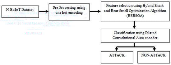
Figure 1.
Block schematic illustration for attack classification.
3.1. Dataset Description
The N-BaIoT database [23] comprises traffic data out of nine Industrial IoTD, whereby seven gadgets gather instances for eleven classes, and the other two gather data for six classes (Ennio_doorbell and Samsung_SNH_1011_N_Webcam). The data consist of harmless traffic and diverse malevolent attacks such as scan, TCP, UDP, and SYN attacks. There remains a sum of eighty-nine csv files in the current database’s variant, having sum dimensions of 7.58 GB and 1,486,418 instances for ordinary and attack happenings. The 2 Bas—MIRAI and BASHLITE—have been classified into ten attack classes (AC) and NA. The AC includes:
- Scan commands for finding the defenseless IoTD;
- ACK, SYN, UDP, and TCP flooding;
- Combo or combination attacks employed to open a link and transmit the spam into this.
3.2. Pre-Processing Employing OhE
A categorical column (CC) is a column containing classes, where the cardinality remains minimum in nature. In the N-BaIoT database, four columns are detected as CCs, specifically ‘Dir’, ‘Proto’, ‘sTos’, and ‘dTos’. The first column comprises seven classes, the second one comprises fifteen classes, the third one comprises six classes, and the fourth one comprises five classes. OhE indicates the procedure of transforming CCs into vectors of zeros and ones. A column with two and three classes has vector lengths of two and three, respectively. Transforming a five-class CC into a vector of zeros and ones with a length of five produces multicollinearity problems (MP).
The MP leads to unnecessary data and associated anticipators. The MP could be resolved by dropping a column’s OhE classes. Thus, a column having five classes possesses a vector length of four rather than five. Relating to N-BaIoT, the OhE columns’ quantity for four CCs would be twenty-nine columns currently. Every categorical feature (CF) exhibiting m feasible categorical values will be converted into a value in Rm employing a function e, which maps the feature’s jth value into the m-dimensional vector’s jth element.
The two arithmetical CFs will be scaled concerning every feature’s average π and standard deviation β:
Pre-processing transforms NT into an observance sequence in which every observance will be portrayed as a feature vector (FV). The observances will be selectively labelled by their class as ‘normal’ or ‘anomalous’. Such FVs will later be appropriate as inputs for data mining or ML algorithms.
3.3. FS Employing HSBSOA
The motivation behind the shark smell optimization (SSO) algorithm is the shark’s capability and supremacy in capturing prey by employing a strong sense of smell (SoS) in a short time. A bear’s olfactory bulb remains many times bigger than the rest of the beasts when its top job is to forward smell data from the nose toward the brain. In the bear smell optimization (BSO) methodology, the bear’s SoS is exemplary in seeking foodstuffs at 1000 miles and beyond (known as the global solution (GS)) in optimization). As bears cannot see foodstuffs that far away, the statistical paradigm centered upon the SoS proposes a decisive manner for seeking such goals. By merging these two algorithms, a better fitness value (FtV) could be acquired for the FS procedure.
3.4. Initialization Procedure
The initial solution (IS) for the SSO algorithm’s (SSOA) populace should be produced haphazardly inside the search space (SSp). Every IS portrays an odor particle (OP) that exhibits a feasible shark location at the start of the search procedure. The IS vector will be illustrated in Equations (3) and (4), accordingly to which refers to the populace vector’s starting location and NP = population size refers to the populace’s dimensions:
The concerned optimization issue could be conveyed by:
where represents the jth size of the shark’s ith location and ND represents the decision variables’ numeral. By employing the BSO methodology, the bear’s nose absorbs disparate smells; every one exhibits a location for movement, since all things possess a distinct odor in the ecosystem. Notice that several of these are called local solutions (LS). The desirable foodstuff’s specific smell remains the final solution and is regarded as the GS. Consider being the ith obtained smell having elements or particles, which is designed to solve the optimization issue . As the bear obtains n smells during the breathing duration, the IS remains a matrix . Presently, as per the glomerular layer procedure and breathing action in a sniff sequence, indicates the jth smell element within ith. Centered upon statistical formulas, we obtain two conditions, which are and with the presence of fairness, which includes the balanced energy to maintain the traffic in the transmission line:
Equation (5) works for the condition , where represents the inhalation time (IT) and denotes the balanced energy required during the inhalation process:
Equation (6) works for the condition , where represents the exhalation time (ET) and denotes the balanced energy required during the process of exhalation. In the optimization procedure, the comprehensive duration of a breathing cycle remains identical to k or the ith smell’s length, and as per the ET and IT the smell elements are split into 2 sets.
The total balanced energy is the summation of the energy required for the processes of vital energy (VE) and energy loss (EL) and is mathematically expressed below:
where denotes the dissipated energy during the process of inhalation and exhalation and denotes the transmission loss that occurs.
3.5. Odor Absorption (OA)
For the process of odor absorption, mitral and granular parts are used to contain the receptor sensitivity, OA, as well as the input data, which are presented as . Presently in this condition, exhibits that there is no smell in the olfactory epithelium prior to the subsequent inhalation. The non-negative array could be computed as:
where k indicates the odor’s extent in ith odor, while Equation (7) works for two conditions, which are the threshold values and , where the arrays centered upon the odors data’s represent the mean value. Here, denotes the satisfaction factor, whereby the mathematical expression for this factor is expressed as:
where N denotes the total number of odor absorption mitral and W denotes the weight factor. The neural dynamics evolving out of the granular and mitral (GM) layers are calculated as:
where and represent the G-M cell (GMC) actions accordingly; and represent the outward inputs to the mitral and middle of the granule cells, respectively; denotes the initial energy and denotes the lowest energy unit.
3.6. Frontward Motion (FtM) toward the Target
If the blood is discharged into the water, a shark possessing a velocity V goes towards the powerful OPs in every position to move nearer to the prey (target). Thus, the velocity within each size will be computed as:
where k = 1, 2, … , which would be the objective function (OF) at location ; indicates the phases’ maximal quantity for the forward motion of the shark, k indicates the phases’ quantity, indicates a value within the interval [0, 1], and is a haphazard number in the interval [0, 1]. The rise in the odor intensity decides the increase in the shark’s velocity. Owing to inertia, the shark’s acceleration remains a constraint. Thus, the present shark’s velocity depends upon its former velocity, which can be utilized by altering (9), as exhibited in the following expression:
where portrays the inertia coefficient within the interval [0, 1], portrays the shark’s former velocity, and , like , remains a haphazard number in the interval [0, 1]. Because of the shark’s FtM, its novel location remains , which is decided depending upon its former location () and velocity (). Hence, the shark’s novel location can be described as:
where i denotes a time interval that can be presumed to be one for simplicity:
| Pseudocode for frontward motion begins Calculate velocity V Update the position of target prey Velocity of each shark () Find maximal quantity for forward motion Release the odor and find its intensity Update the shark’s novel location End |
3.7. Rotatory Motion (RM)
The shark also possesses an RM that will be employed to discover powerful OPs. The SSOA procedure can be named the local search (LcS), which can be defined as:
in which , and denotes a haphazard number in the interval [−1, 1]. In the LcS, several points (M) will be linked to create closed contour lines and to design the shark’s RM within the SSp.
3.8. Updating the Particle Location
The shark’s search path will carry on with the RM, since this is nearer to the point of having a powerful SoS. This feature within the SSOA could be described by:
in which portrays the shark’s subsequent location with the greatest OF value.
3.9. Attaining GS and LS
In the process of attaining GS and LS at the initial stage, two values are determined, which are , and the expression for this is given below:
The expressions and indicate the GMC accordingly; and portray the GMC’s time constants, and their values remain as 0.14; and simulate the cell output actions for the GMCs. Thus, we can obtain:
In both Equations (18) and (19), the term represents the threshold value, and the values of and are 0.14 and 0.29, respectively. Here, the synaptic-strength connection matrices are calculated, which are represented as , , and , which indicate the association between the GMCs and the mitral cells. This is computed as:
, , and indicate the connection constants, rand() indicates a haphazard value, indicates the space between the ith and gth odors based on their data, and the gth odor indicates the desirable odor for the bear; that is to say, this distance can be described between every odor (LS) and the intended odor (GS). This exhibits that the supervised operation centered upon the GS will be utilized while performing the optimization procedure to enhance the exploitation. As per the above-mentioned explanations, if the brain acquires all data from the neural action, the disjoining procedure is centered upon the discrepancy analysis. This procedure will be simulated while centered upon the Pearson correlation. Hence, this point assists the bear in choosing the finest manner for the subsequent location. The probability odor components (POC), probability odor fitness (POF), and odor fitness (OF) are described by:
where denotes the lower and upper limits of the odor components. The mathematical expression for the calculation of is described as:
where are the lower and upper limits of the odor components, respectively. The discrepancy between 2 odors can be computed using the expected odor fitness (EOF) and distance odor component (DOC) formulas as:
where g denotes the GS. The values of the odor fitness (EOF) and distance odor components (DOCs) are measured according to Equations (19) and (20), where the distances of the probability odor components (POC) and probability odor fitness (POF) are considered. The mathematical expressions for the calculation of are given below:
where the distances between the source and destination coordinates are used for the calculation of the distances of POC and POF; denotes the source coordinates and denotes the destination coordinates.
These expressions denote the feasible manner shift. Indeed, these indices describe the association between the odors that have been reached at the desirable location. It is legibly exhibited that the brain’s output determines an appropriate manner for the subsequent location. In the mesh grid region, the distance between entire odors can be centered upon 2 THs.
In this phase, the HSBSOA can be employed to extract the finest features. Initially, the shark and bear’s beginning locations will be located to be in the middle of the data. Next, the fitness or finesse is noted for every position surrounding the shark and bear by employing the fitness function. Then, the HSBSOA will be implemented to extract the finest features. In this study we extracted twenty-one features via the HSOSOA out of every datapoint by implementing twenty-one repetitions. Every repetition possesses just one feature extracted with the greatest FtV. While performing each repetition, the shark and bear’s positions will be updated to be frontward or rotatory-centered upon the FtV. When the position’s FtV in the shark position’s FM remains above the shark RM’s FtV, the shark’s location will be updated. The shark’s trajectory will move frontward or rotatory depending upon the position’s FtV; additionally, the positions that will be viewed using the HSBSOA can be reviewed.
| Pseudocode: HSBSOA Algorithm Begin: Initialize search space Indicate the total number of populations Compute the optimization issue Compute decision variables numeral Compute local solution (LS) from decision variable Update the inhale and exhale parameter Update exhalation time (ET), inhalation time (IT) Initiate Odor absorption Compute non-negative array Compute granular and mitral (G-M) layers Initiate Frontward motionCompute velocity V for each shark Update for all location Find shark’s acceleration Initiate Rotatory motion Compute local search (LcS) Updating the particle location Compute probability odor components Compute probability odor fitness (POF) Find the fitness parameter End |
3.10. Classification Employing DCAE
Before introducing DCAE, for detailed comprehension, it remains notable that the notation ‘dilated convolution’ (DC) portrays a convolution procedure with a dilated filter (DlF). Generally, the DC is implemented in the wavelet decomposition discipline. As the DC operant solely employs a similar filter at disparate scales having disparate dilation factors (DtF), its application in no way encompasses the DlF’s formation. In addition, the dilated convolutional network can extend the receptive field (RF) dimension, which depends upon enhancing the DtF instead of expanding the network’s field map (FMp) dimensions.
The layers involved in the process of the ACAE framework are the input layer, convolutional layer, DC layer, flatten and reshape layer, recurrent layer, and then finally the output layer as shown in Figure 2. The dilated convolutional layer is incorporated with a filter size of (3, 3) and with a dilation size of (1, 2, 4). In order to process the dilation in the mathematical order, the discrete function is given as , while the size of the discrete filter is mentioned as . The math expression for the calculation of the DC operator © is given below:
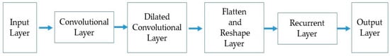
Figure 2.
ACAE framework.
In Equation (28), the term X represents (x − g), Y represents (y − h), and , which is the discrete filter with a size of . Here, denotes the corresponding integer index value, which lies between (0 to 5) and , denoted as the entropy loss calculation, which lies between 0 and 10.
Secondly, an improved dilation convolution is developed with the variants . The math expression for the calculation of the improved DC operator is given below.
Thus, the convolutions © and are called one-DC. Here, we presume that for the remaining DFs and for the remaining 3 × 3 DsFs. Furthermore, the filters are implemented by aggressively enhancing DtFs such as . Next, the DF could be conveyed as:
Similarly:
As per the RF description, two sections are present for every component, which are and . The terms and are the constant values that are used for experimental purposes and which satisfy the condition ( + ). The math expression for the combined detection methodology is given below:
Thus, RF remains a square of aggressively enhanced dimensions. In the convolutional layers (CvLs), the former layer’s FMs will be convolved with multiple convolutional kernels (CKs), especially FMp. Next, the independent layer’s outcomes added with a bias will be supplied to an activation function (AF) to create an FM. Presuming that remains a value at the row for channel within the FM of the layer, the value of could be acquired as:
where refers to a hyperbolic tangent function for ; specifically, are the biases for the FM (i, j), g refers to the present FM linked to the layer, and refer to a value at location p within CK to which the dimensions are while the terms are the objective functions.
For the initial block, every CvL layer will be incorporated by (1) a CL that convolves its inputs with an array of kernels to be learnt in the training stage, (2) a rectified linear unit (ReLU) layer that maps convolved outcomes by the function , and (3) a normalization layer that normalizes values of disparate FMs in the former layer. The math expression for is given below.
In Equations (35) and (36), the terms k, α, and β remain the hyper-criteria, and G(i) and G(j) remain the FMs’ array-incorporated terms during normalization. The ensuing 3 layers remain DC layers, having disparate dilated factors. For example, in this study we consecutively selected one, two, and four.
For the next block, centered upon the former exposure, the depth of a minimum of 2 recurrent layers remains advantageous for processing the concatenative data. This study utilizes a 2-layer stacked LSTM. Moreover, a ReLU will be used as the AF. The dropout layer is implemented in the LSTM layer’s input for regularization. Furthermore, recurrent batch normalization is employed to lessen the internal covariance shift amidst the time phases.
The next block remains a completely linked network layer. This remains akin to a conventional multilayer perceptron neural network (NN), which maps the latent features into the output classes (OC). In this layer, the softmax function is described below:
Next, an entropy cost function will be incorporated, centered upon the probabilistic outcomes and the training instances’ actual labels. In the course of the training stage, all the criteria will be modified to search for the minimal cost. Additionally, a sliding window (SW) scheme will be utilized to segment the time sequence signal into signals’ small pieces. In particular, an instance employed by the CNN remains a 2D matrix comprising r unprocessed samples (with every sample having D features). In this way, r will be selected to remain as the sampling rate or the finite duration, and the SW’s phase dimension will be selected to retain a fifty percent overlap between the nearby windows. Hence, the shorter phase dimension remains the instances’ bigger quantity that experiences greater calculative workloads. Furthermore, the signals’ small portion will be generally very frequently labelled.
| Pseudocode: Proposed Approach Begin five classes = CC categorical feature (CF) = Rm, e Compute average π Compute standard deviation β Find Check the shark’s capability Capture the prey EmploySoS Initiate the smelling process Achieve global solution Find the fitness value Indicate the total number of population Compute the optimization issue Compute decision variable numeral Compute local solution (LS) from decision variable Update the inhale and exhale parameter Update exhalation time (ET), inhalation time (IT) Initiate Odor absorption Compute Compute non-negative array Compute granular and mitral (G-M) layers Calculate velocity V Update the position of target prey Velocity of each shark () Find maximal quantity for forwarding motion Release the odor and find its intensity Update the shark’s novel location Initiate Frontward motion Compute velocity V for each shark Update for all locations Find shark’s acceleration Initiate Rotatory motion Compute local search (LcS) Update the particle location Compute probability odor components Compute probability odor fitness (POF) Find the fitness parameter Stop |
4. Performance Analysis
The dilated convolutional classifier-based botnet detection method (HSBSOpt_DCA) is implemented in Python 3.7 using the Ubuntu 16.04 operating system with 8 GB of RAM. The database chosen for the feature selection is the N-BaIoT database, which includes the traffic data for nine industrial IoTD. Seven databases are the gadgets’ gathered instances for eleven classes, and two are the gadgets’ gathered data for six classes (Ennio_doorbell and Samsung_SNH_1011_N_Webcam). The experimental outcome will be assessed by measuring the performance matrices, such as the accuracy, precision, recall, and F1-score. Such criteria will be correlated with four advanced methodologies: CNN-related SS for DD and its identification (CNN-SSDI), the bidirectional LSTM model (BI_LSTM), ODNN, and RPCO_BCNN with the proffered HSBSOpt_DCA.
4.1. Performance Matrices
- Accuracy: This provides the capability for comprehensive anticipation generated by the paradigm. The true positive (TP) and true negative (TN) give the ability to anticipate the intrusion’s existence or non-existence. The false positive (FP) and false negative (FN) provide the false anticipation given by the employed paradigm. The mathematical expression for the calculation of the accuracy is described as [15]:
- Precision: Precision is defined as the positive output achieved by the algorithm used in the proposed model, which lies in the range of (0 to 1). It computes the intrusion classification paradigm’s victory. It defines the classifier’s probability for anticipating the outcome as positive if the intrusion exists. It is as called the TP rate. It can be measured as:
- Recall: This is the classifier’s probability of anticipating the outcome as negative if the intrusion does not exist. It is also known as the TN rate, as mentioned below:
- F1-Score: This is used to measure the anticipation execution. It is defined as the weighted mean calculation of the precision and recall. The F1-score lies between 0 and 1. If the score is 1, it is considered the most acceptable value; if it is 0, it is regarded as weak. The mathematical expression for the calculation of the F1-score [15] is given below:
4.2. Results and Discussion
In this section, the metrics such as the accuracy, precision, recall, and F1-score are measured with respect to 50 and 100 epochs. Each metric calculation on the various epochs is evaluated. The accuracy calculations with variable epochs numbering 50 and 100 are demonstrated in Figure 3 and Figure 4.
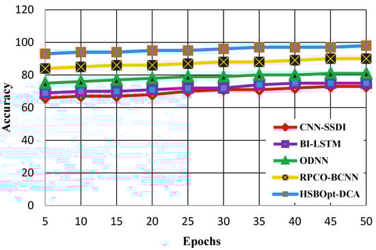
Figure 3.
Accuracy calculation with 50 epochs.
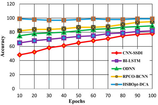
Figure 4.
Accuracy calculation with 100 epochs.
Figure 3 shows the accuracy calculation for methods such as the CNN-SSDI, BI_LSTM, ODNN, RPCO_BCNN, and HSBSOpt_DCA. It can be understood from Figure 3 that the proposed HSBSOpt_DCA produces better accuracy when compared with other methods with respect to the 50 epochs. Various levels of accuracy are achieved by the CNN-SSDI (73%), BI_LSTM (75%), ODNN (81%), RPCO_BCNN (90%), and HSBSOpt_DCA (98%) methods. The accuracy achieved by the proffered HSBSOpt_DCA method is high and is achieved by using the hybrid optimization and dilated convolution process.
Figure 4 shows the accuracy calculation for methods such as CNN-SSDI, BI_LSTM, ODNN, RPCO_BCNN, and HSBSOpt_DCA. The figure proves that the proffered HSBSOpt_DCA method produces better accuracy than the other methods for 100 epochs. The accuracy scores achieved by the methods vary for CNN-SSDI (78%), BI_LSTM (82%), ODNN (89%), RPCO_BCNN (95%), and HSBSOpt_DCA (99%). The accuracy achieved by the proffered HSBSOpt_DCA method is high using the hybrid shark and bear smell optimization algorithm.
The precision calculations with 50 and 100 epochs are demonstrated in Figure 5 and Figure 6. Figure 5 shows the precision calculation for methods such as CNN-SSDI, BI_LSTM, ODNN, RPCO_BCNN, and HSBSOpt_DCA. The figure proves that the proffered HSBSOpt_DCA method produces better precision when compared with the other methods for 50 epochs. The precision scores achieved by the methods vary for CNN-SSDI (58%), BI_LSTM (69%), ODNN (75%), RPCO_BCNN (93%), and HSBSOpt_DCA (99%). The precision achieved by the proffered HSBSOpt_DCA method is high using the hybrid shark and bear smell optimization algorithm.
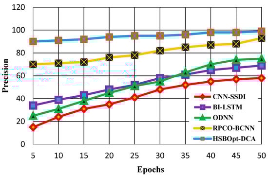
Figure 5.
Precision calculation with 50 epochs.
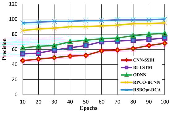
Figure 6.
Precision calculation with 100 epochs.
Figure 6 shows the precision calculation for methods such as CNN-SSDI, BI_LSTM, ODNN, RPCO_BCNN, and HSBSOpt_DCA. The figure proves that the proffered HSBSOpt_DCA method produces better precision when compared with the other methods for 100 epochs. The precision scores achieved by the methods vary for CNN-SSDI (68%), BI_LSTM (75%), ODNN (81%), RPCO_BCNN (95%), and HSBSOpt_DCA (99.9%). The precision achieved by the proffered HSBSOpt_DCA method is high using the hybrid shark and bear smell optimization algorithm.
The recall calculations with 50 and 100 epochs are demonstrated in Figure 7 and Figure 8. Figure 7 shows the recall calculation for methods such as CNN-SSDI, BI_LSTM, ODNN, RPCO_BCNN, and HSBSOpt_DCA. The figure proves that the proffered HSBSOpt_DCA method produces better recall than the other methods for 50 epochs. The recall scores achieved by the methods vary for CNN-SSDI (85%), BI_LSTM (81%), ODNN (85%), RPCO_BCNN (85%), and HSBSOpt_DCA (91%). The recall achieved by the proffered HSBSOpt_DCA method is high and is achieved by using the hybrid optimization and dilated convolution process.
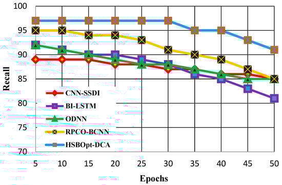
Figure 7.
Recall calculation with 50 epochs.
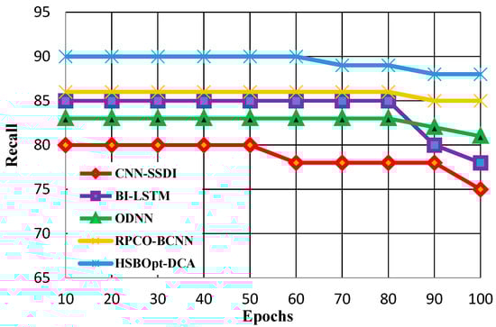
Figure 8.
Recall calculation with 100 epochs.
Figure 8 shows the recall calculation for methods such as CNN-SSDI, BI_LSTM, ODNN, RPCO_BCNN, and HSBSOpt_DCA. The figure proves that the proffered HSBSOpt_DCA method produces better recall than the other methods for 100 epochs. The recall scores achieved by the methods vary for CNN-SSDI (75%), BI_LSTM (78%), ODNN (81%), RPCO_BCNN (85%), and HSBSOpt_DCA (88%). The recall achieved by the proffered HSBSOpt_DCA method is high and is achieved by using the improved dilated convolution process.
The F1-score evaluations for 50 and 100 epochs are demonstrated in Figure 9 and Figure 10. Figure 9 shows the calculation of the F1-scores for the proposed and existing methods. The figure proves that the proffered HSBSOpt_DCA method produces a better F1-score than the other methods for 50 epochs. The F1-scores achieved by the methods vary for CNN-SSDI (73%), BI_LSTM (75%), ODNN (81%), RPCO_BCNN (94%), and HSBSOpt_DCA (98%). The F1-score achieved by the proffered HSBSOpt_DCA method is high and is achieved by using the improved dilated convolution process.
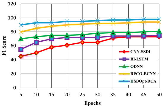
Figure 9.
F1-score calculation with 50 epochs.
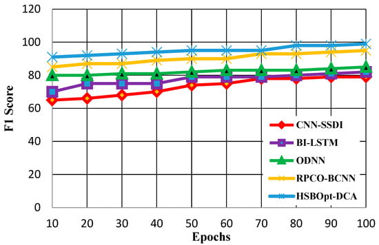
Figure 10.
F1-score calculation with 100 epochs.
Figure 10 shows the calculation of the F1-scores for the proposed and existing methods. The figure proves that the proffered HSBSOpt_DCA method produces a better F1-score compared with other methods for 100 epochs. The F1-scores achieved by the methods vary for CNN-SSDI (79%), BI_LSTM (82%), ODNN (85%), RPCO_BCNN (95%), and HSBSOpt_DCA (99%). The F1-score achieved by the proffered HSBSOpt_DCA method is high and is achieved by using the improved dilated convolution process. Therefore, it is evident from the experiments that the proposed approach outperforms other existing methods, and it can be concluded that the feature extraction using the optimization algorithms definitely increases the performance of the classification model; therefore, the model can be used to detect and classify security threats in FANET.
5. Conclusions
In this study, we proposed an effective model combining hybrid shark and bear smell optimization (HSBSOA) to secure the FANET from security threats. It provides a solution to investigate the FANET botnet detection threat and to solve the combinational optimization problem. Then, a dilated convolution autoencoder classifier is employed to detect and classify the security threats in the network. The parameters considered for the performance analysis of the proffered HSBOpt_DCA are the accuracy, precision, recall, and F1-score. Moreover, the performance of the proposed approach was compared with CNN-SSDI, bi_LSTM, ODNN, and RPCO-BCNN. The performance of the proposed HSBOpt_DCA network was evaluated with different epochs. The proposed model with 50 epochs achieved 98% accuracy, 99% precision, 91% recall, and a 98% F1-score. For 100 epochs, it achieved 99% accuracy, 99.9% precision, 88% recall, and a 99% F1-score. The comparison showed that the proposed HSBOpt_DCA achieved 33% better accuracy, 30% better precision, 13% better recall, and a 20% better F1-score than the existing methods. The proposed method provides a global security solution to the security issues in the UAV-FANET framework. The proposed hybrid-optimization-based feature selection process reduced the computational time. It achieved higher accuracy, precision, recall, and F1-scores than the existing approaches. However, the classification tasks still require improvement, which can be considered in the future.
Author Contributions
Conceptualization, N.F.A., F.A., H.M.A.G., S.K. and A.A.; methodology, N.F.A. and A.A.; software, N.F.A. and A.H.A.; validation, A.H.A., A.S.A. and A.A.; formal analysis, N.F.A.; investigation, A.S.A.; resources, A.H.A.; data curation, M.H.H. and F.H.A.; writing—original draft preparation, A.A. and A.H.A.; writing—review and editing, S.K.; supervision, A.H.A. and S.K. All authors have read and agreed to the published version of the manuscript.
Funding
The research received no external funding.
Data Availability Statement
Not Applicable.
Acknowledgments
This work was supported by the Ministry of Science and Higher Education of the Russian Federation (Government Order FENU-2020-0022).
Conflicts of Interest
The authors declare no conflict of interest.
References
- Gupta, S.; Sharma, N.; Rathi, R.; Gupta, D. Dual Detection Procedure to Secure Flying Ad Hoc Networks: A Trust-Based Framework; Springer: Singapore, 2021; Volume 210, pp. 83–95. [Google Scholar] [CrossRef]
- Jasim, K.S.; Alheeti, K.M.A.; Alaloosy, A.K.A.N. A Review Paper on Secure Communications in FANET. In Proceedings of the 2021 International Conference of Modern Trends in Information and Communication Technology Industry (MTICTI), Sana’a, Yemen, 4–6 December 2021; 146, pp. 1–7. [Google Scholar] [CrossRef]
- Bekmezci, İ.; Şentürk, E.; Türker, T. Security issues in flying ad-hoc networks (FANETS). J. Aeronaut. Space Technol. 2016, 9, 13–21. [Google Scholar]
- Dadi, S.; Abid, M. Enhanced Intrusion Detection System Based on AutoEncoder Network and Support Vector Machine; Springer: Singapore, 2021; Volume 466, pp. 327–341. [Google Scholar] [CrossRef]
- Rodrigues, M.; Pigatto, F.D.; Fontes, J.V.C.; Pinto, A.S.R.; Diguet, J.-P.; Branco, C.K. UAV Integration IntoIoIT: Opportunities and Challenges. In Proceedings of the 13th International Conference on Autonomic and Autonomous Systems (ICAS 2017), Barcelona, Spain, 21–25 May 2017; p. 95. [Google Scholar]
- Bekmezci, I.; Sahingoz, O.K.; Temel, Ş. Flying Ad-Hoc Networks (FANETs): A survey. Ad Hoc Netw. 2013, 11, 1254–1270. [Google Scholar] [CrossRef]
- Sang, Q.; Wu, H.; Xing, L.; Xie, P. Review and Comparison of Emerging Routing Protocols in Flying Ad Hoc Networks. Symmetry 2020, 12, 971. [Google Scholar] [CrossRef]
- Hussain, A. A Hybrid and Robust Delay and Link Stability Aware (DLSA) Routing Protocol for Unmanned Aerial Ad-Hoc Networks (UAANETs). Res. Sq. 2021; Preprint (Version 1). [Google Scholar] [CrossRef]
- Zafar, W.; Khan, B.M. A reliable, delay bounded and less complex communication protocol for multicluster FANETs. Digit. Commun. Netw. 2017, 3, 30–38. [Google Scholar] [CrossRef]
- Walia, E.; Bhatia, V.; Kaur, G. Detection Of Malicious Nodes in Flying Ad-HOC Networks (FANET). Int. J. Electron. Commun. Eng. 2018, 5, 6–12. [Google Scholar] [CrossRef]
- Yanmaz, E.; Costanzo, C.; Bettstetter, C.; Elmenreich, W. A discrete stochastic process for coverage analysis of autonomous UAV networks. In Proceedings of the 2010 IEEE Globecom Workshops, Miami, FL, USA, 6–10 December 2010; 40, pp. 1777–1782. [Google Scholar] [CrossRef]
- Ahamed S, M.J.; Krishnamoorthy, J. Cyber threats based on botnet and its detection mechanisms. In Proceedings of the 8th Annual International Research Conference, Oluvil, Sri Lanka, 25 November 2019. [Google Scholar]
- Verma, S.; Sharma, N.; Singh, A.; Alharbi, A.; Alosaimi, W.; Alyami, H.; Gupta, D.; Goyal, N. DNNBoT: Deep Neural Network-Based Botnet Detection and Classification. Comput. Mater. Contin. 2022, 71, 1729–1750. [Google Scholar] [CrossRef]
- Fried, A.; Last, M. Facing airborne attacks on ADS-B data with autoencoders. Comput. Secur. 2021, 109, 102405. [Google Scholar] [CrossRef]
- Mall, P.; Amin, R.; Obaidat, M.S.; Hsiao, K.-F. CoMSeC++: PUF-based secured light-weight mutual authentication protocol for Drone-enabled WSN. Comput. Netw. 2021, 199, 108476. [Google Scholar] [CrossRef]
- Mairaj, A.; Javaid, A.Y. Game theoretic solution for an Unmanned Aerial Vehicle network host under DDoS attack. Comput. Netw. 2022, 211, 108962. [Google Scholar] [CrossRef]
- Popoola, S.I.; Ande, R.; Adebisi, B.; Gui, G.; Hammoudeh, M.; Jogunola, O. Federated Deep Learning for Zero-Day Botnet Attack Detection in IoT-Edge Devices. IEEE Internet Things J. 2021, 9, 3930–3944. [Google Scholar] [CrossRef]
- Hatzivasilis, G.; Soultatos, O.; Chatziadam, P.; Fysarakis, K.; Askoxylakis, I.; Ioannidis, S.; Alexandris, G.; Katos, V.; Spanoudakis, G. WARDOG: Awareness Detection Watchdog for Botnet Infection on the Host Device. IEEE Trans. Sustain. Comput. 2019, 6, 4–18. [Google Scholar] [CrossRef]
- Xi, R.; Hou, M.; Fu, M.; Qu, H.; Liu, D. Deep Dilated Convolution on Multimodality Time Series for Human Activity Recognition. In Proceedings of the 2018 International Joint Conference on Neural Networks (IJCNN), Rio de Janeiro, Brazil, 8–13 July 2018; pp. 1–8. [Google Scholar] [CrossRef]
- Alharbi, A.; Alsubhi, K. Botnet Detection Approach Using Graph-Based Machine Learning. IEEE Access 2021, 9, 99166–99180. [Google Scholar] [CrossRef]
- Sung, Y.; Jang, S.; Jeong, Y.-S.; Park, J.H. Malware classification algorithm using advanced Word2vec-based Bi-LSTM for ground control stations. Comput. Commun. 2020, 153, 342–348. [Google Scholar] [CrossRef]
- Shitharth, S.; Prasad, K.M.; Sangeetha, K.; Kshirsagar, P.R.; Babu, T.S.; Alhelou, H.H. An Enriched RPCO-BCNN Mechanisms for Attack Detection and Classification in SCADA Systems. IEEE Access 2021, 9, 156297–156312. [Google Scholar] [CrossRef]
- Dua, D.; Graff, C. UCI Machine Learning Repository. 2019. Available online: https://archive.ics.uci.edu/ml/datasets/detection_of_IoT_botnet_attacks_N_BaIoT (accessed on 5 June 2022).
Publisher’s Note: MDPI stays neutral with regard to jurisdictional claims in published maps and institutional affiliations. |
© 2022 by the authors. Licensee MDPI, Basel, Switzerland. This article is an open access article distributed under the terms and conditions of the Creative Commons Attribution (CC BY) license (https://creativecommons.org/licenses/by/4.0/).