A Holistic Scalability Strategy for Time Series Databases Following Cascading Polyglot Persistence

Abstract

Time series databases aim to handle big amounts of data in a fast way, both when introducing new data to the system, and when retrieving it later on. However, depending on the scenario in which these databases participate, reducing the number of requested resources becomes a further requirement. Following this goal, NagareDB and its Cascading Polyglot Persistence approach were born. They were not just intended to provide a fast time series solution, but also to find a great cost-efficiency balance. However, although they provided outstanding results, they lacked a natural way of scaling out in a cluster fashion. Consequently, monolithic approaches could extract the maximum value from the solution but distributed ones had to rely on general scalability approaches. In this research, we proposed a holistic approach specially tailored for databases following Cascading Polyglot Persistence to further maximize its inherent resource-saving goals. The proposed approach reduced the cluster size by 33%, in a setup with just three ingestion nodes and up to 50% in a setup with 10 ingestion nodes. Moreover, the evaluation shows that our scaling method is able to provide efficient cluster growth, offering scalability speedups greater than 85% in comparison to a theoretically 100% perfect scaling, while also ensuring data safety via data replication.

1. Introduction

The extraordinary advancement in the technological field has led to a significant explosion in the amount of generated data, in turn, raising interest in obtaining further knowledge from it [1]. This phenomenon goes to the extent that time series databases, aimed to handle the information coming from continuous data sources such as sensors, has been the fastest growing database category since 2019 [2].

Following the aim of further facilitating time series data management, NagareDB was born. NagareDB targets a different objective that most popular databases, as it does not intend to provide the fastest performance at any cost, but the best balance between resources consumption and performance [3]. In order to lower barriers to sensor data management, NagareDB materialized a Cascading Polyglot Persistence approach, which has shown not only to reduce the needed software and hardware resources, but also to outperform popular databases such as MongoDB and InfluxDB.

Cascading Polyglot Persistence follows a complex time-oriented nature, where several data models complement each other in the handling of time series data. More precisely, it makes sensor readings flow from one data model to another until reaching the last one, data being present in one single data model at a time.

Although Cascading Polyglot Persistence showed to greatly improve the database performance, it was only tailored to monolithic architectures, relying on third-party general approaches for scaling out in a cluster fashion. Consequently, Cascading Polyglot Persistence approaches could in fact be deployed among different machines in a collaborative way, but the scaling approach was not suited to the nature nor the goal of Cascading Polyglot Persistence itself, missing the opportunity of maximizing its efficiency.

As the monitoring infrastructures’ market is growing day by day, monolithic approaches that consist of a single machine are not always able to handle all use cases. More precisely, back-end data infrastructures are typically requested to consist of several machines, either for performance reasons or due to data safety concerns. Consequently, it becomes necessary for every database to provide a tailored and specific scaling approach aimed to maximize its performance and to strengthen its goal.

In this research, we propose an ad hoc scalability approach for time series databases following Cascading Polyglot Persistence. However, we do not intend to provide a fixed approach, as each use case holds its particular requirements involving data consistency, fault tolerance, and many others. Consequently, we propose a flexible one that can be tailored to the specifics of each scenario, together with further analysis and performance tips. Not only that, we analyze the behaviour and performance of the approach given different possible setups according to both real-time and near real-time data management. Thus, our flexible approach intends to facilitate the tailoring of the cluster to each different use case while further improving the system performance.

More precisely, our approach aims to correlate each data model of Cascading Polyglot Persistence to a very specific setup and configuration, both in terms of software and hardware. This holistic approach intends to extract the whole potential of Cascading Polyglot Persistence, fitting it even more naturally to the infrastructure of each deployment scenario.

After analysing the approach with different cluster setups, from one to three ingestion nodes, and from 1 to 100 ingestion jobs, the approach showed to be able to offer a scalability performance up to 85%, in comparison to a theoretically perfect 100% performance, while also ensuring data safety by automatically replicating the data in different machines. Indeed, it has shown to be able to write up to 250,000 triplet data points per second, each composed of a time stamp, a sensor ID, and a value in a cluster setup composed of machines allocated with poor resources, such as 3 vCPUs, 3 GB of RAM, and a solid disk drive of just 60 GB.

Thus, our approach demonstrated that fast results can be obtained not only by powerful and expensive machinery, but also thanks to use-case tailored resources and efficient strategies.

2. Background

2.1. CAP Theorem

When dealing with distributed systems, such as a database in a cluster fashion, it becomes essential to understand and deal with the CAP theorem [4]. This theorem makes selecting data management systems that better fit the characteristics and requirements of an application easier and helps users understand the problems that might occur when dealing with a distributed environment.

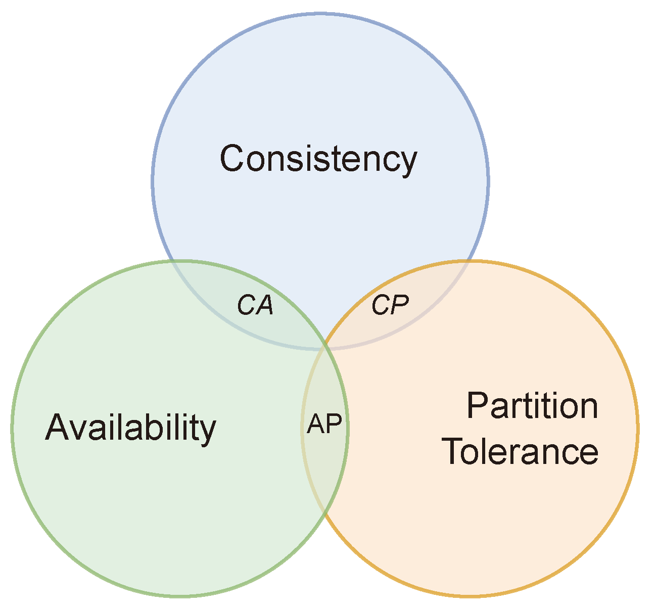
The CAP theorem, also called Brewer’s Conjecture, states that a distributed system can deliver only two of the three commonly desired properties: consistency, availability, and partition-tolerance, affirming that it is not possible to achieve all three, as represented in Figure 1.

Consistency. It means that all database clients will always see the same data, regardless of the cluster machine or node that they are connecting to.

Availability. This property means that any client making a request to the data management system will always obtain a response, even in the case that one or more nodes of the cluster are down, as long as the node that received the request is running correctly.

Partition Tolerance. It means that when a cluster suffers from a partition, a communication break between two nodes, the system should be able to continue working, despite the number of partitions that the system suffered.

2.2. Scalability Approaches

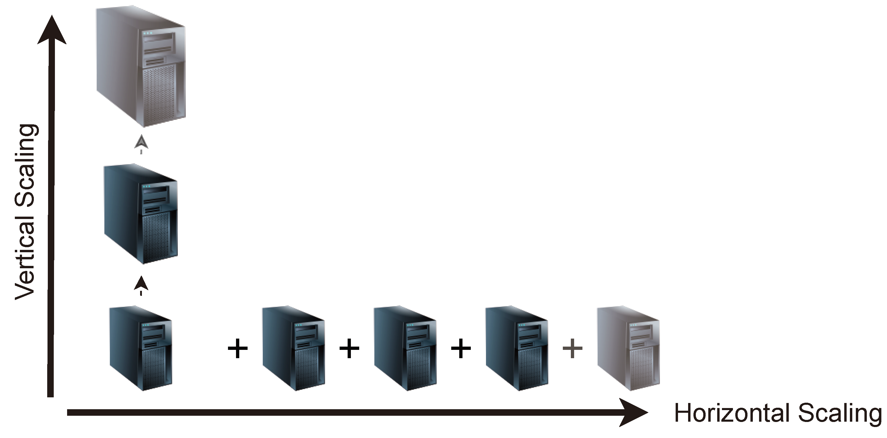
While some use cases might find it enough to follow a static approach, in terms of computing resources, more demanding scenarios, either in terms of storage, performance, availability, or capacity planning, are likely to need a more sophisticated setup. In order to overcome the limitations of a given machine, applications such as databases are typically requested to scale along with the hosting machinery. There are several approaches to pursue that growth, as represented in Figure 2:

Vertical Scalability. When performing vertical scalability, or scaling up, the infrastructure keeps the same setup but increases its specifications. As the infrastructure remains the same, there is no need to modify any configuration or database client code. The database is not distributed among different machines (or at least not more than previously) but just running in a setup with more resources than prior to the scaling.

Horizontal Scalability. Thanks to scaling horizontally, or scaling out, databases are able to work in a distributed environment. The performance no longer resides in a single-but-powerful machine but in a set of different machines that could be commodity ones. Thus, the data and load are distributed across different machines that work together as a whole.

2.3. Cluster Techniques

In the context of this research, the most relevant scalability techniques involving the creation of a cluster, such as horizontal scalability, are: sharding, replication, and their combination.

2.3.1. Sharding

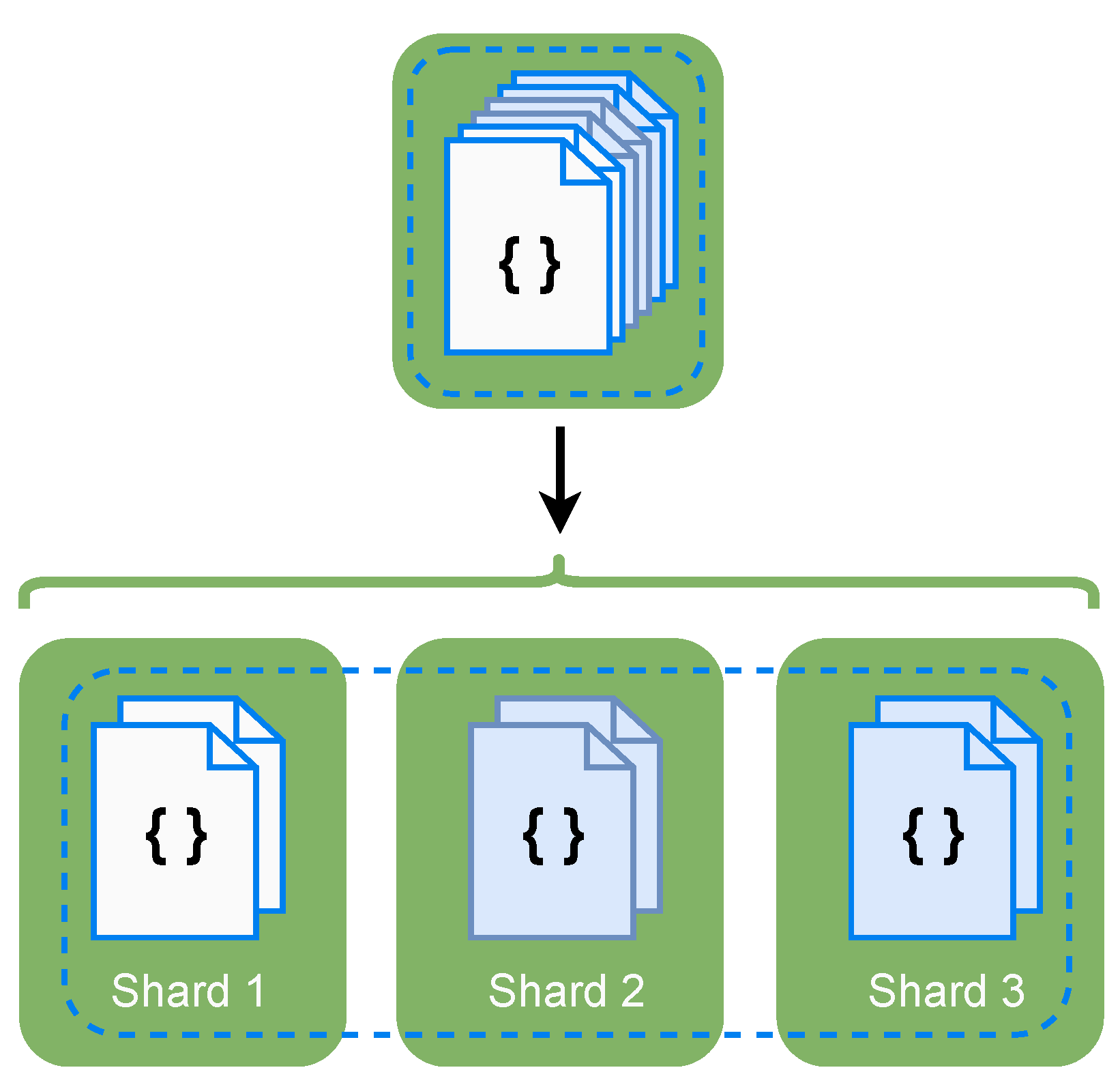
It is a database architectural pattern associated with horizontal scalability. As seen in Figure 3, when sharding, data are divided across different instances of the database, typically in different machines.

This database fragmentation enables data to be stored and distributed across the cluster. However, there are some disadvantages of solely performing sharing. For example, if one shard is down, when performing queries that involve data of that shard, phenomenons such as wrong query answering are likely to happen. For instance, queries will return partial or incomplete results. Thus, it is not possible to assume that the query was answered correctly, as important information will be missing.

On the other hand, if the database is set up to avoid wrong query answering, when a node or shard becomes unavailable, the whole database will be compromised, and every query against the database will be discarded or blocked until the missing shard becomes available. This reduced availability effect is increased when sharding because the more machines there are in a cluster, the more likely one of them will suffer an issue.

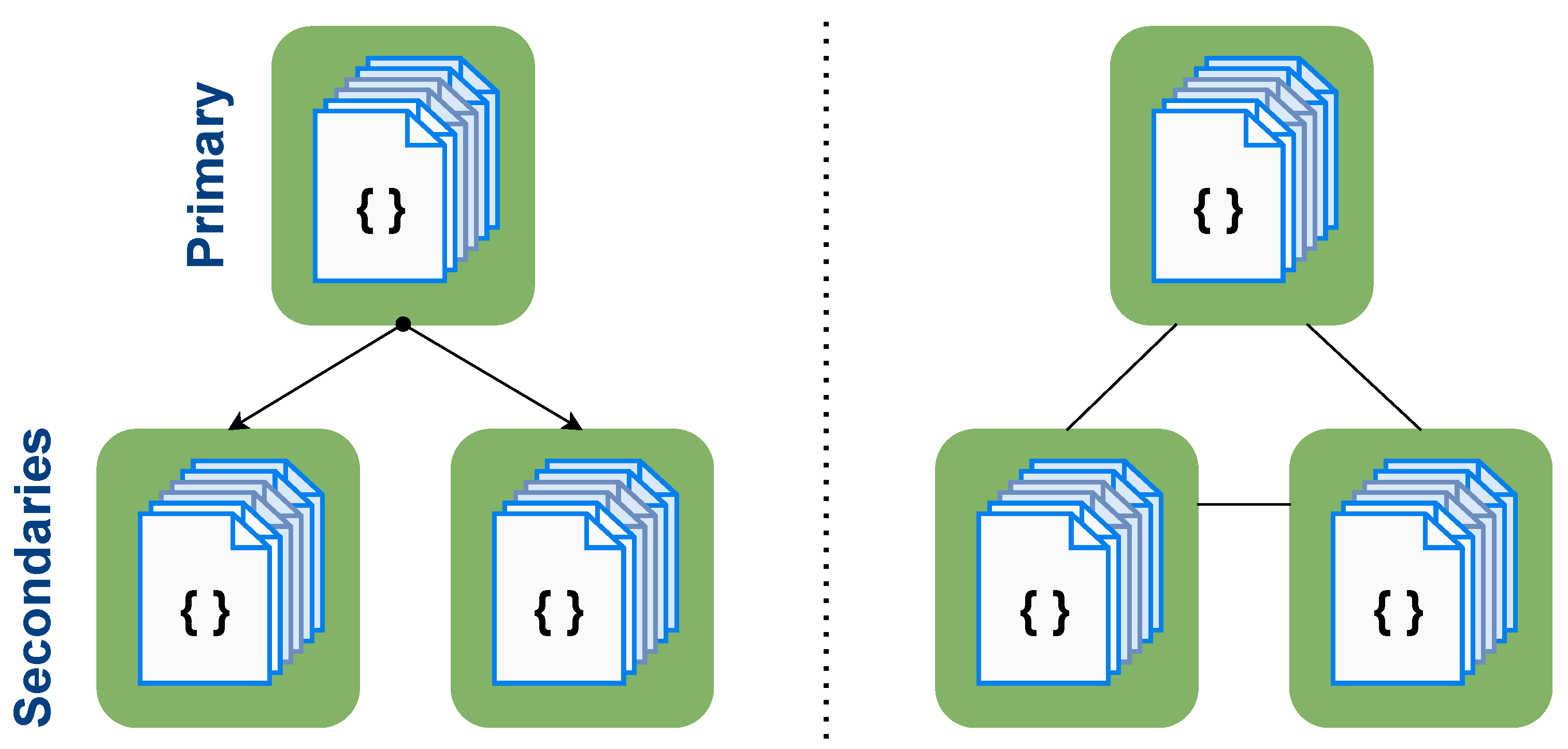
2.3.2. Replication

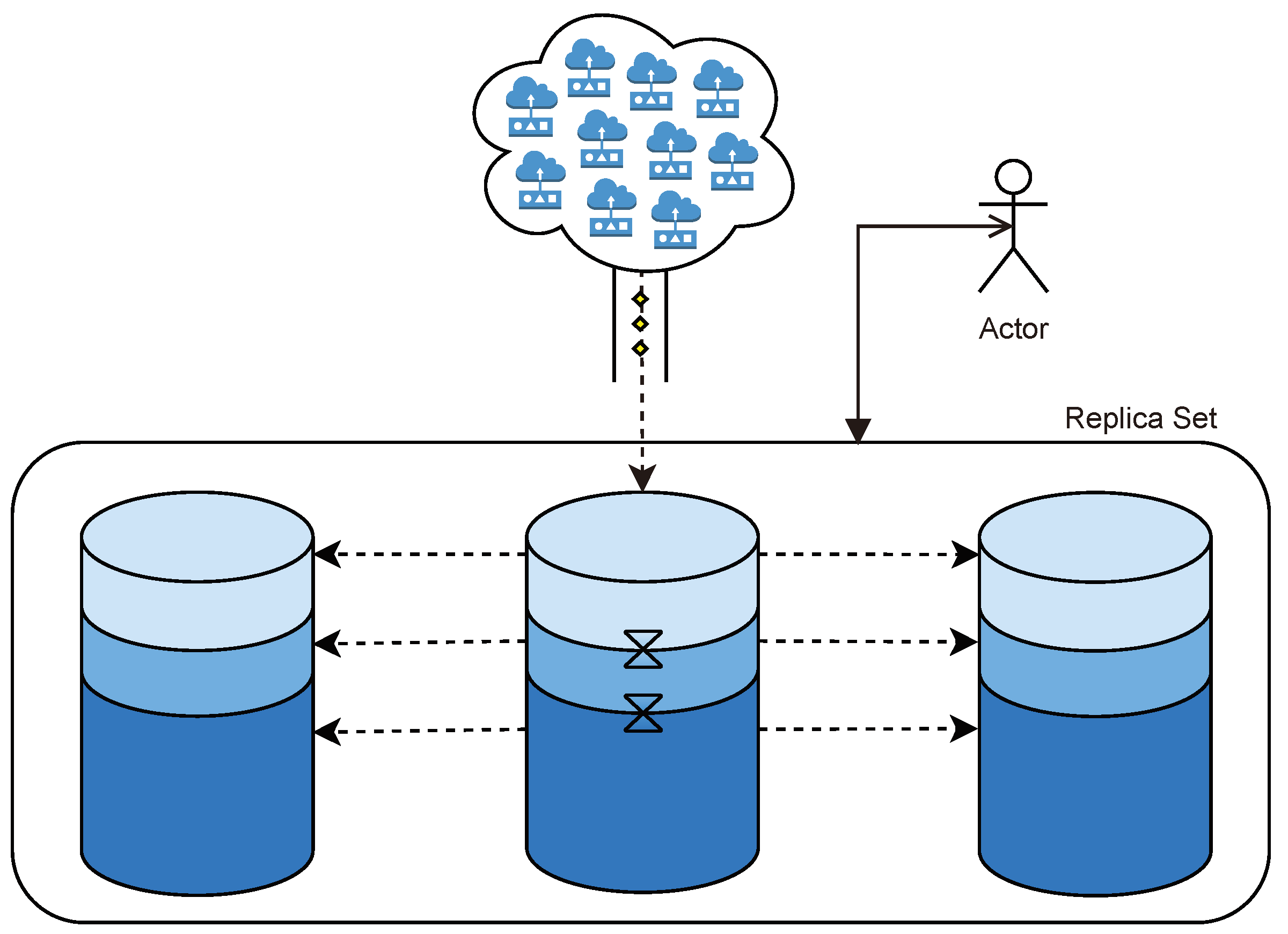
Data replication is the process of creating several copies of a given dataset across different instances or machines in order to make the data more available and the cluster more reliable. Figure 4 represents two replica sets that ensure partition tolerance. So, two groups of instances that have the same data, where the replication factor is three, imply that the very same data will be replicated three times in the cluster.

On the one hand, to avoid consistency issues, thus following an AP approximation of the CAP theorem, each replica set of size N is typically composed of a primary instance and N-one secondary instance. Write operations are performed directly to the primary instance for being replicated to the secondary instances later. This restriction makes the primary instance the main access point to the system which ensures consistency. In the situation where the primary instance becomes unavailable, a secondary instance will take the role of the primary one, temporarily receiving all write operations. In the meantime, after the primary instance is compromised but before the secondary instance takes its role, the system will not be available for any write operation, as, in fact, it follows a CP approximation, missing the availability property.

On the other hand, to avoid availability issues, replica sets can be configured so that all members have equal responsibilities. When following the AP approximation of the CAP theorem, all nodes are able to read and write data, making all nodes equally important. Thus, if a node fails, queries are able to be straightforwardly redirected to another node. However, as all nodes ingest different data, for its later synchronization, consistency is compromised as there is no guarantee that all nodes will have the same data.

However, although replication brings recovery capabilities and improves data availability, among others, it has an important drawback. The bigger the replica set is, the more available it will be, but it will also cost more. For instance, if the replication factor is set to three, three machines will be holding the same data, which implies the hardware and maintenance costs will be tripled, dramatically increasing the budget requirements.

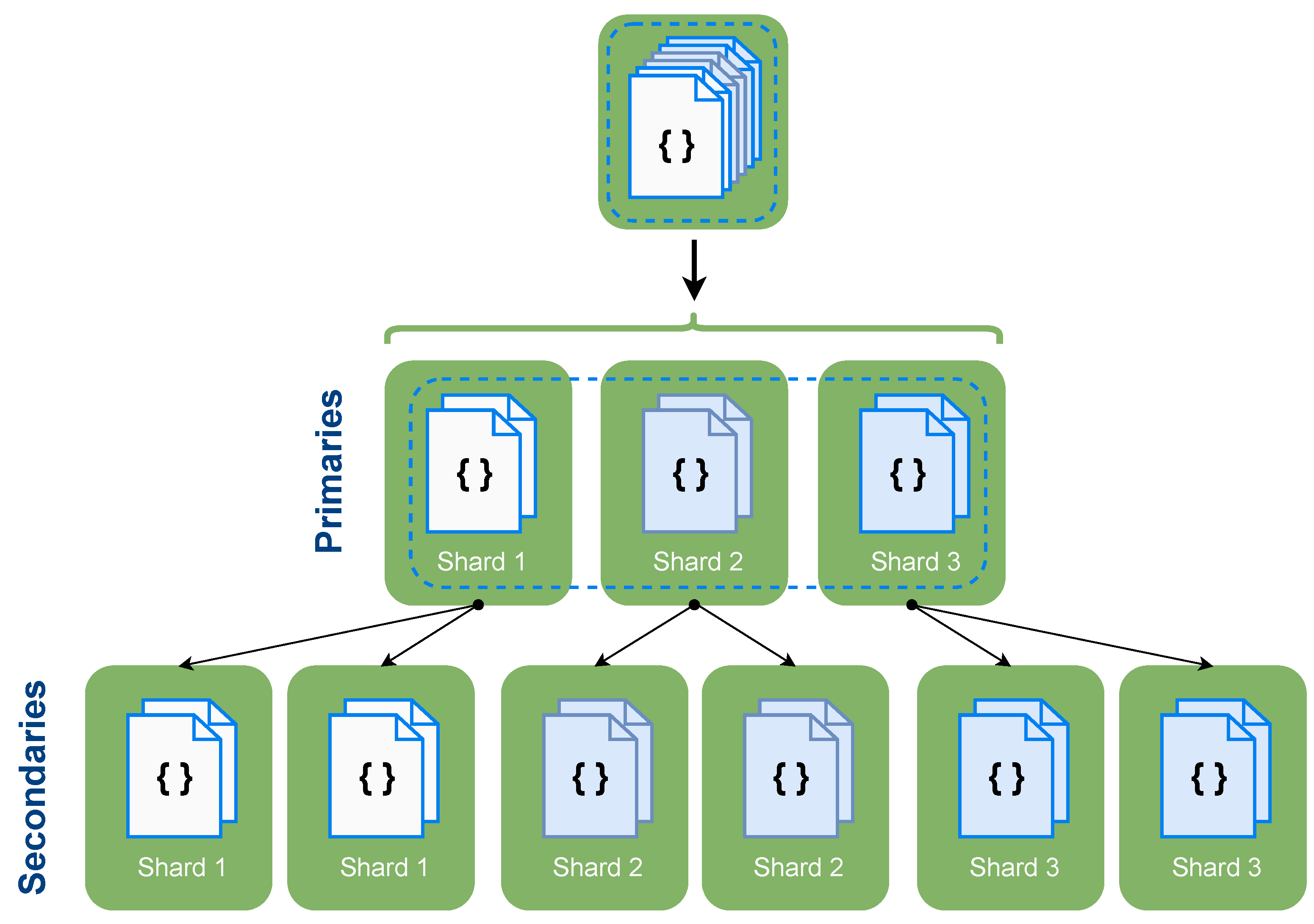
2.3.3. Sharding and Replication

As explained in Section 2.3.1, sharding is able to increase the system capabilities and resources. However, it does not come free of inconvenience as it is at the expense of compromising the data availability. In the opposite direction, replication is aimed at improving data availability. Thus, it is noticeable that replication is able to compensate the issue that sharding causes. As a consequence, both sharding and replication techniques are likely to collaborate, creating a cluster composed of shards and replica sets.

As seen in Figure 5, when combining replication and sharding, sharding typically divides or fragments the database, and replication is aimed to replicate those separated shards, improving their availability. However, while replication is able to compensate the main problem of sharding, replications’ drawback—the increased infrastructure costs—is still an issue.

2.4. Data Compression

Since the amount of data to be kept is limited by the storage resources, data compression techniques capable of reducing the storage requirements while keeping the same amount of data play a relevant role in time series databases.

However, compressing real-time data has an important drawback, as it is not computationally free, meaning that it typically reduces the I/0 throughput, trading CPU time for this reduced storage consumption [5,6].

As a consequence, it becomes important not only to choose the technique that offers the best compression ratio, but also to find a good trade-off between the CPU overhead produced by the compression. Some of the most relevant lossless compression techniques in the context of this research are:

Snappy. It does not aim for the maximum compression but for a fast compression/decompression and a reasonable compression ratio [7]. It is able to process data in an order of magnitude faster for most inputs in comparison to other compression techniques, such as ZLIB. However, as a consequence, its compression ratio falls behind both Zstd and Zlib [6].

Zlib. It is a general-purpose lossless data-compression library [8]. It is able to provide superior compression ratios [5], while also being suitable for real-time compression due to its acceptable compression latency [9]. However, its compression and decompression speed falls far behind other compression algorithms, such as snappy or zstd [6].

Zstd. It is a fast lossless compression algorithm, whose target focuses on real-time compression scenarios [6]. It offers a good compression ratio, being similar to the one of Zlib in some scenarios, while providing a faster compression speed in all cases, slightly slower than fast compressors such as snappy [6,9].

2.5. Disk Drives

In recent years, disk drives have experienced a dramatic evolution in order to meet new challenges and demands. This game-changing breakthrough has directly impacted database management systems, whose cornerstone is typically its persistence devices. In the context of this research, the most relevant technologies associated to disk drives are:

Hard Disk Drives (HDD). They are electromechanical devices, as the information is stored on a spinning disk covered with ferromagnetic material [10]. Thus, as the disk has to physically rotate, applications that have to read or write data in a random fashion are heavily penalized. In contrast, applications that have to read or write data sequentially obtain a good disk performance [11]. Their ratio storage/price ratio is typically outstanding, making them an affordable option for persisting data [12].

Solid-State Drives (SSD). As they are solid drives, they lack from any moving mechanical part [13], which greatly improves the reading and writing speed of data. However, they still offer much less capacity per drive in comparison to HDDs, making them relatively more expensive in terms of storage/price ratio [12]. There are a wide range of different SSD devices, each with a different interface connector and a different speed to offer. For instance, ntraditional SSD devices, which typically rely on a SATA 3 interface, are able to offer speeds up to 600 MB/s, whereas SSD devices that rely either on NVMe M.2 or a PCIe 3.0 interfaces are able to offer speeds up to 3900 MB/s. Ultimately, the latest SSD devices implementing new interfaces such as PCIe 4.0 are able to reach up to 8000 MB/s, leaving not just traditional HDDs, but also its SSD siblings far behind. However, these stunning speed improvements, especially regarding last generation SSDs, come associated with high purchasing costs [12], becoming almost prohibitive for some modest environments.

2.6. Data Organization

Databases’ performance is not only affected by the way data are physically stored or persisted, but also by the structure of the data that is being sent to the database and retrieved from it [14]. As explained in Section 1, this research will also dig into this phenomenon and into how it interacts with the approaches explained in Section 2.2. In order to facilitate the reading of the concepts that will follow, this section summarizes the three most relevant data organizations in the context of this research:

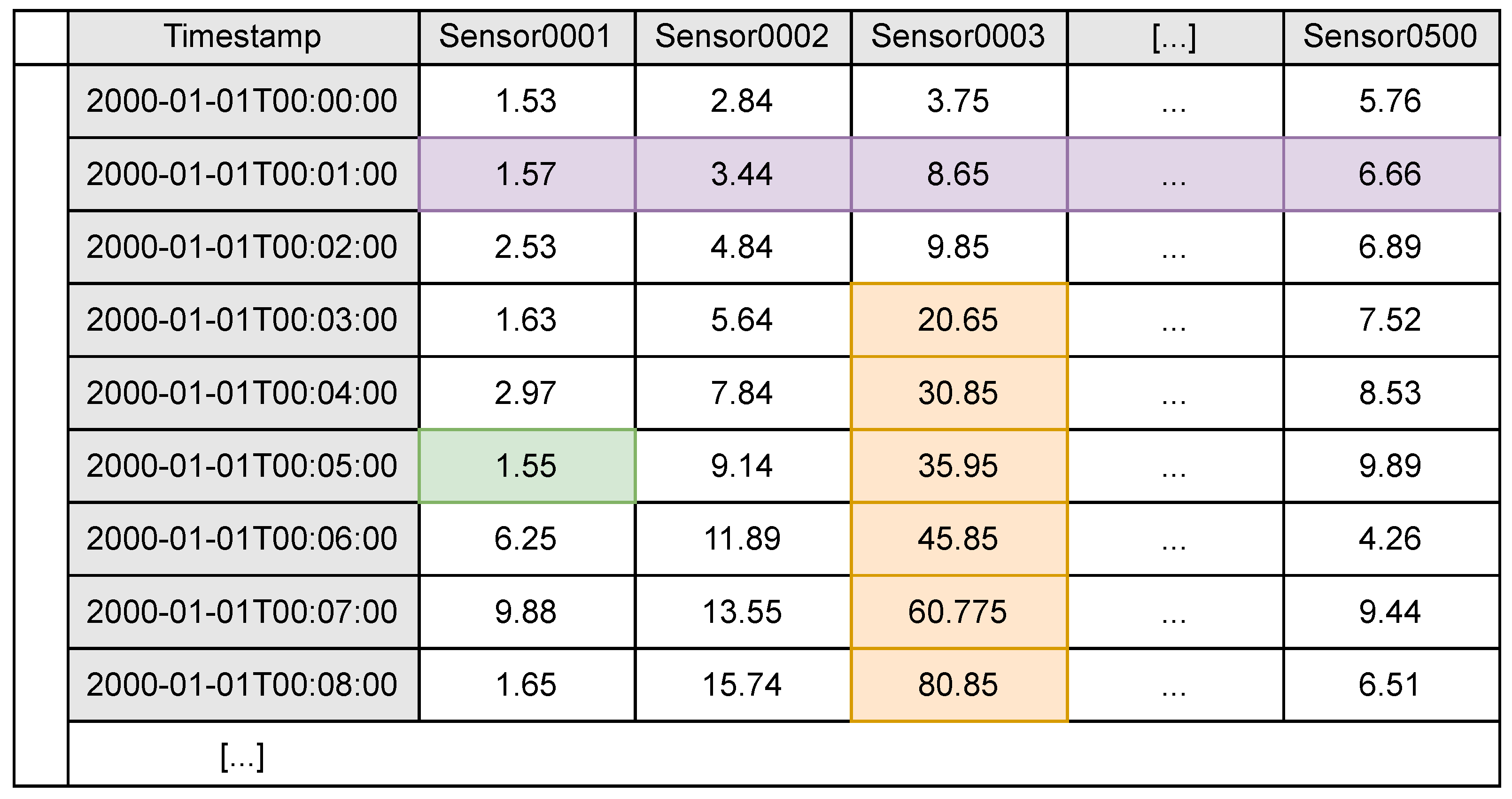
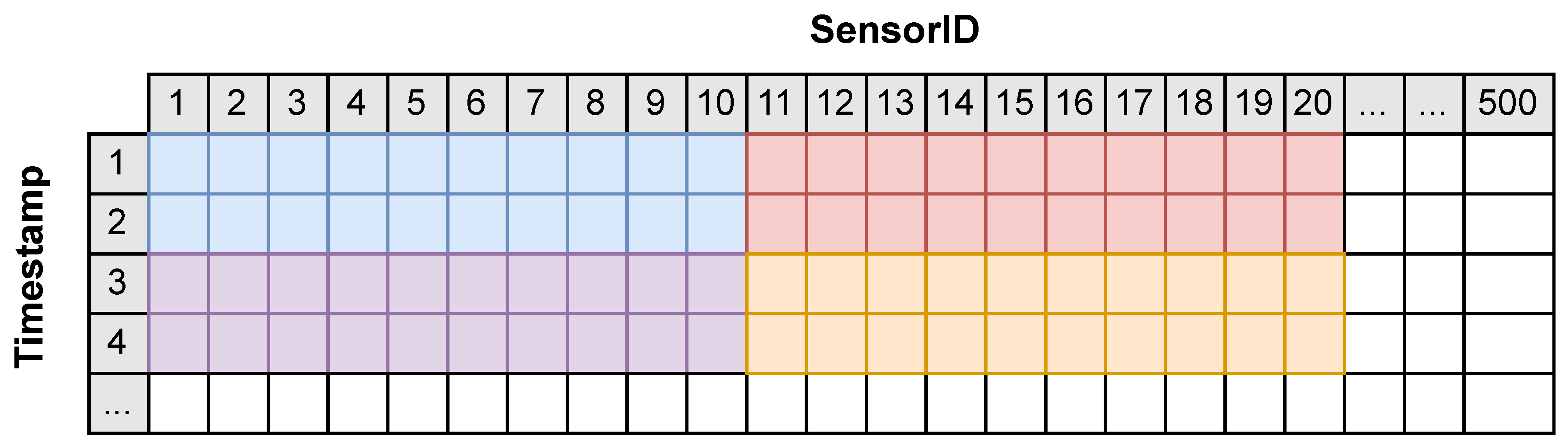
Triplet. It is the most granular record in a time series database, presented in an independent fashion. It is a data structure composed of three different elements: the ID of the sensor that reads the data, a time stamp of the instant that it was read, and a value representing the reading. A triplet sample can be seen in Figure 6, with value 1.55.

Row. It groups triplets that share a time stamp, regardless of their sensorID. A full row could be divided into other rows, making them share the same time stamp but each has a different subset of sensorIDs. A full row sample can be seen in Figure 6, colored in purple. It is composed of all the triplets that share the time stamp 2000-01-01T00:01:00.

Column. It groups triplets that share the same sensorID, regardless of their time stamp. It is typically incomplete since having a full column would mean possessing all information for any existing time stamp. Thus, it typically has a starting time stamp and a latest time stamp, which delimit the column length. A column sample can be seen in Figure 6 colored in orange. It holds the sensor reading of sensor Sensor0003 between 2000-01-01T00:03:00 and 2000-01-01T00:08:00.

3. Related Work

This section describes related solutions involving time series databases aimed at handling sensor data management. More precisely, it describes some of the most relevant solutions in the context of this research, their different approaches for tackling scalability, the best practices that they recommend to follow when dealing with clusters, and how they relate to the CAP theorem, among others.

3.1. MongoDB

It is the most popular NoSQL database [15,16]. It provides an extremely flexible data model based on JSON-like documents [17]. However, although its aim is to provide a general purpose but powerful database, since mid-2021 with MongoDB 5.0, it also provides a specific purpose capability aimed to handle time series data. Thanks to this capability, MongoDB is able to work either as a general purpose database or as a time series database [18]. Given that MongoDB is a broadly known database, this new capability is able to further lower the barriers to access time series databases, as finding experts in MongoDB, and its query language, is easier that in any other specific purpose database [2].

MongoDB stores all time series data in a single set of documents by default [18]. Moreover, it uses an approximation to a column-oriented data model embedded on top of its document-based data structure [19]. This eases the usage of the database itself, as the basic persistence model does not vary with respect to MongoDBs’ document-based capabilities, while it also improves historical querying due to its column-oriented approximation [14,20]. However, in terms of performance, it falls far behind other time series database solutions, while it typically consumes more disk resources [14].

Regarding its scalability offer, MongoDB enables the database to scale out even in its community edition version. More precisely, MongoDB globally provides two different patterns: sharding and replication. Thanks to them, the database is able to grow in a cluster fashion, adding more machines and resources to the distributed database as explained in Section 2.3.

On the one hand, when sharding, MongoDB advocates for uniformly distributing the data across the different shards, as explained in the MongoDB’s Sharding Manual [17]. More precisely, data are grouped in chunks—a continuous range of shard keys, with default size of 64 Mb—and each chunk is assigned to a different shard, aiming to avoid uneven distributions and migrating chunks from one shard to another if necessary. The shard key, the element MongoDB uses to distribute data, can be chosen by the database administrator, which makes it possible to distribute data according to the time stamp, according to the sensorID, or any other metadata.

On the other hand, when performing replication, MongoDB offers it in a instance-wise basis. This means that it is not possible to replicate a single shard but just a whole instance of the mongo daemon. Thus, if a machine holds a MongoDB instance and the instance holds several shards, it is not possible to replicate a single shard.

This makes the cluster work in two different fashions at the same time: chunk-wise for sharding and instance-wise for replication. In order to ensure data availability, as explained in Section 2.3, MongoDB clusters typically materialize both scalability approaches simultaneously.

Last, regarding its guarantees as a distributed data store, according to the CAP theorem explained in Section 2.1, MongoDB mainly behaves by default following the CP approach. This makes MongoDB assure data consistency and partition tolerance while compromising availability. More precisely, this is due to the fact that when acting as a distributed database, MongoDB by default does not allow a user to query secondary instances, only primary ones [17]. In the case of a failure on the primary one, it will not be possible to interact with the system until a secondary one takes the role of a primary one. If MongoDB allowed users to query secondary instances, in case of failure, the system would be query-able, but it would probably return inconsistent results (behaving as an AP), as there is no guarantee that the secondary would have the exact same data as the primary.

3.2. InfluxDB

It is the most popular time series database [2]. InfluxDB follows a column-oriented data model [21], able to efficiently reduce historical data disk usage while also providing outstanding historical querying speed [14,22]. InfluxDB internally organizes and groups its data according to several factors, such as the retention policy of the data itself—the maximum time that it will remain in the system before removed—the measurement type, and other metadata [21]. This way of organizing data in groups that share several properties allows it to efficiently query time series data within the same group and to offer an outstanding compression. However, this constant grouping implies several overheads when querying data that belong to different groups [14], both when retrieving and ingesting data, and also determines and limits the way in which the database is able to grow.

More precisely regarding scalability, InfluxDB is only able to grow in a cluster fashion in its enterprise edition. This implies that the free and open source version of the database is only able to work in a monolithic environment, limiting itself to vertical scalability approaches. When scaling using its enterprise edition, InfluxDB is able to grow following the shard-replica technique, explained in Section 2.3. However, due to its particular way of storing and understanding time series data, its sharding technique has several specificities. For instance, InfluxDB is designed around the idea that data are temporary, meaning when each element of data enters the system, it is already known when it is going to be removed. This is not an exception to shard, as they are linked to a retention policy, meaning that data will only live a certain duration, which is by default always less than 7 days [21]. When reaching the duration of a shard, a new one will be created. This approach is particular to InfluxDB, as shards will be constantly being created in contrast to techniques such as the one of MongoDB that establishes a fixed amount of shards that do not have to be linked to a retention policy. Finally, both original and replica shards are uniformly distributed across the cluster, aiming to also distribute their load.

Regarding its replication approach particularities, InfluxDB treats primary instances and secondary instances in a more similar way than other databases such as MongoDB. For instance, when querying a shard that has been replicated, the query does not have to be answered by the primary shard. Rather, it can be answered by a randomly chosen one [23]. This mechanism is able to improve querying speed, as they can be distributed to several machines instead of being handled by a fixed one. However, this brings further issues with respect to consistency, as there is no guarantee that all the replicas will have the same data. This design approach makes InfluxDB belong to the AP approach of the CAP theorem, as it is able to provide availability and partition tolerance, but there is just a limited guarantee of consistency.

3.3. NagareDB

NagareDB is a time series database built on top of MongoDB 4.4 CE, a fact that lowers its learning curve, as it inherits most of its capabilities and its popular query language. In contrast to other databases, NagareDB’s goal is not to obtain the fastest results at any cost but to provide a good trade-off between efficiency and resource usage. Thus, it aims to democratize time series database approaches, intending to offer a fast solution that is able to run in commodity environments.

Following its cost-efficient philosophy, but aiming to further maximize performance, NagareDB recently introduced an approach called Cascading Polyglot Persistence. Thanks to this approach, the database, referred to as PL-NagareBD, is not just tailored to time series data but also (1) to the natural flow of time series data from ingestion, to storage, until retrieval, (2) to the expected operations according to data aging, and (3) to the format and structure in which users want to retrieve the data [14]. Mainly, it was defined “as using multiple consecutive data models for persisting data of a specific scope, where each data element is stored in one and only one data model at the same time, eventually cascading from one data model to another, until reaching the last one” [14].

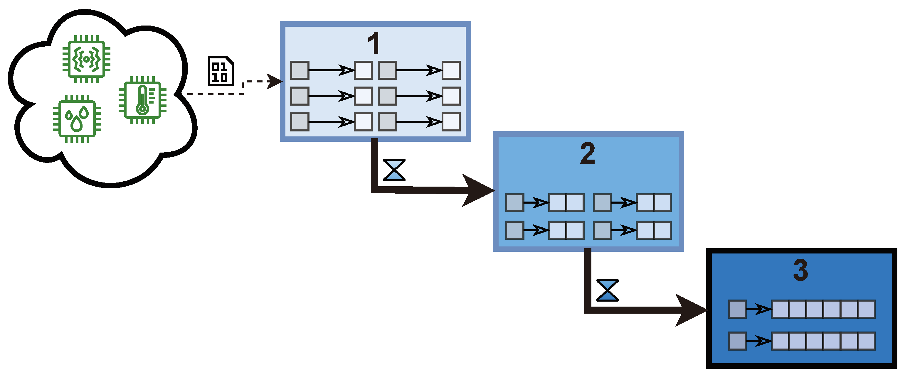
This new paradigm for handling time series data implies that the data store is split into several parts and data models, while being requested to act as a whole in an uniform way as a single logical database. In addition, data are expected to remain in a data model a certain amount of configurable time. For instance, when using three data models, as explained in Figure 7, data are stored by default one day in the first data model and one month in the second one until reaching the last data model where it will remain. Thus, data are requested to eventually cascade from one data model to another, altering their structure. This difficulty, however, can be substantially lightened if Cascading Polyglot Persistence is implemented in a multi-model database, such as NagareDB, able to handle several data models at the same time, which has shown to transform data requesting just a trifling amount of time [14]. Moreover, Cascading Polyglot Persistence comes accompanied with Polyglot Abstraction Layers, which relieves the user from handling the different data models and their internal representations. Thus, the user interacts with a uniform layer in a general and simple data model without having to worry about the internal data representation and whether data are persisted in a data model or in another.

NagareDB, when implementing Cascading Polyglot Persistence, has demonstrated not only to beat MongoDB but also to globally surpass InfluxDB, the most popular time series database, both in terms of querying and ingestion, while requesting a similar amount of disk. More precisely, the approach was able to solve queries up to 12 times faster than MongoDB and to ingest data 2 times faster than InfluxDB among others.

However, while NagareDB’s new approach has shown promising results, the architecture is not accompanied by an efficient and effective way of scaling, relying on classical scalability approaches inherited by MongoDB, leaving a big space for further improvements in cluster-like setups.

3.4. Conclusions

In this section, we analyzed the two typical mechanisms for horizontal scalability: sharding and replication, plus some of the most relevant databases, in the context of this research: MongoDB, InfluxDB and NagareDB under Cascading Polyglot Persistence.

To sum up, all three solutions offer different approaches for tackling time series data. First, MongoDB offers a specialization of its broadly known and free database, which makes it easier for any database engineer to use their solution. However, it suffers from low performance and high disk consumption. Second, InfluxDB is the most popular time series database although its global popularity is far behind MongoDB’s. Its data model offers a fast way to query historical data, an outstanding reduced disk usage, but a limited ingestion speed in some circumstances. Its scalability mechanisms are efficiently tailored to the way the database treats the data; however, they are limited to the enterprise paid version. Last, Cascading Polyglot Persistence, when implemented in data stores such as NagareDB, offers an excellent performance able to surpass InfluxDB in both querying and ingestion while using a similar disk space. However, it lacks from specific scalability methods, relying on MongoDB’s inherited ones, a fact that minimizes its potential when deploying in a distributed environment.

Our goal is to overcome the problems associated with the above technologies, proposing a method for handling time series data in a distributed environment, able to provide a fast and resource-efficient solution, and lowering barriers to the handling of time series data.

4. Proposed Approach

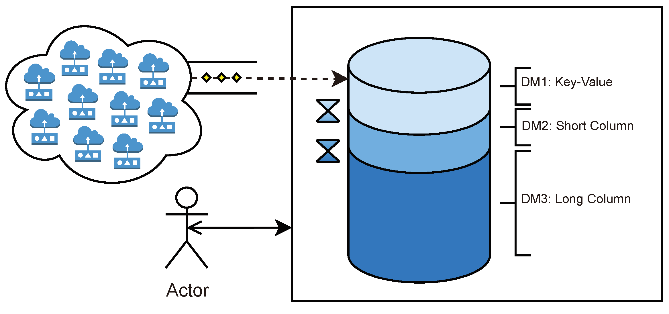
As explained in Section 3, Cascading Polyglot Persistence was intended to provide data stores with a technique to efficiently handle time series data, not only in terms of query performance, but also in terms of resource-saving. It was introduced and evaluated by dividing the database into three different interconnected parts: The first one was in charge of maximizing the ingestion performance, the last one aimed at providing a fast historical querying, and the intermediate one to provide a hybrid and intermediate solution between the other two, as drawn in Figure 8.

However, while other time series solutions offered ad hoc scalability approaches, as explained in Section 3, Cascading Polyglot Persistence lacked from a specific growing method, relying on general approaches, such as the one represented in Figure 9, missing the opportunity to further extract its performance.

Here we introduce the holistic approach aimed at providing Cascading Polyglot Persistence with a scalability mechanism tailored to time series data expected to offer further benefits with respect to resource usage and minimizing hardware deployment costs, while offering efficient scaling.

The main principle of our approach follows the same philosophy of Cascading Polyglot Persistence: specialization. Traditional approaches uniformly distribute data across the different shards or machines. In order to balance the load, each shard does the very same job as any other. In this approach, however, each replica set and their respective shards are grouped according to their data model and, hence, according to their expected usage. This means that data will no longer be distributed uniformly but to a given specific shard according to Cascading Polyglot Persistence. For instance, some shard groups will be in charge of ingestion through Data Model 1, whereas other instances will be in charge of holding historical data, all within the same logical database. Thus, each shard can be configured specifically for improving a particular job or function, also according to the data model that they implement. Last, it is important to recall that, following the same goal as Cascading Polyglot Persistence, one of the main objectives of this approach is to reduce costs while maximizing performance.

Thus, following a sample Cascading Polyglot Persistence approach composed of three data models, such as the one represented in Figure 7, the ad hoc scalability approach divides the cluster into two different replica sets, each holding different properties.

4.1. Ingestion Replica Set—DM1

The first data model of Cascading Polyglot Persistence is intended to improve data ingestion, while also providing excellent performance on short queries [14]. The ability to speedily ingest data are crucial for time series databases, as the vast majority of operations against them are actually write operations [24]. Moreover, DM1 does not intend to keep data a long time, as its default duration is one day. After that, data will be flushed to the next data model in the cascade. Thus, the main goal of scaling out this data model is to provide further ingestion performance.

Taking into account this objective, the Ingestion Replica Set is characterized by the following tightly interrelated properties:

• Diagonal Scalability. When sharding, the cluster could reduce its availability. As explained in Section 2.3, this drawback is compensated for thanks to replication. However, replication introduces a further issue: excessive need of machines. This approach aims at relieving this problem, combining both horizontal and vertical scalability, and looking for a good trade-off, thus, scaling diagonally. More precisely, primary ingestion shards will grow horizontally, each shard in one machine, but their replicas will be hosted together in machines following vertical scalability. Each machine hosting secondary shards, however, will have a maximum number of shards to host according to its resources limitation. If the number of maximum shards is reached, another machine will be added growing horizontally, repeating the process. This intends to reduce the number of machines within the cluster, while still providing good performance, as primary shards, the ones who ingest data, do not have to share resources.
• Sensor-Wise Sharding. When sharding, data are divided across the different shards. However, the way in which data are assigned to a shard or another is not trivial. In this approach, data are divided and grouped according to the original source or sensorID. This approach is way different to the one followed by other databases such as InfluxDB, where sharding is performed time-wise, for instance, creating a new shard according to a given duration. However, sharding sensor-wise has a main benefit. Data ingestion can be parallelized efficiently and straightforwardly, as ingestion is performed in all shards simultaneously. By contrast, if sharding according to time, all sensor data will be shipped to the same shard, the one storing the current day, missing the opportunity to use all available resources. The opposite happens when querying a record history of a given sensor. As all sensor data will be in the same shard, it will not benefit from parallelization. However, historical queries are typically executed against old historical data. Given these characteristics, also considering that Data Model 1 is mainly intended to improve ingestion performance and will only keep as much as one day of data to be retrieved when querying, a sensor-wise sharding strategy is preferred.
• Targeted Operations. They use a given key to locate the data. As data will be distributed sensor-wise, the shard key will also be scattered sensor-wise, meaning that each shard will receive a specific range of sensorIDs. Thanks to this predefined fixed distribution, the query router is able to ship queries and data speedily to the specific shard where they belong. This property is intended to avoid broadcast operations, where a given query in sent to all available shards, causing network overhead. Moreover, broadcast operations typically cause scatter gather queries so queries that are scattered to all shards, whether hosting the data or not, merge all results.
• Eventual Consistency. The Ingestion Replica Set will follow an intermediate approximation between CP and AP of the CAP theorem. By default, the database guarantees consistency (CP), as the router directly queries the primary node, which is always up-to-date, as explained in Section 3. However, it is also possible to query the secondary node if specifically requested. This means that in the situation that the primary node becomes unavailable, the system itself will be always available for readings through the secondary node. In addition, it is also possible to query the secondary node just for load balancing purposes. However, when doing that, there is no guarantee that the data are consistent, as it can be the case that the primary node failed before synchronizing with the secondary one. This flexibility allows the system to offer the best from CP, while also providing a limited AP approach under certain circumstances. This adjustment is related to the time series data nature. Time series data are typically immutable, meaning that data are added but never updated except when done manually. Thus, this eventual consistency just implies that when querying a secondary, the last inserted elements might still not be visible within some milliseconds time range, which makes it fair enough to be traded for availability.
• Reduced Write Concern. The database write concern is set up to one acknowledgement. This means that each insert operation will be considered successful when it is acknowledged by the primary shard without waiting until being replicated to the secondary one(s). This property improves system speed as operations have to wait less time to be completed and enables secondary shards to copy data from the primary in a batch-basis, relieving them from excessive workloads and making efficient use of the CPU, disk, and network resources. As all secondary shards will be hosted in the same machine due to diagonal scalability, this property is crucial as it prevents vertical hosts that hold several shards to saturate. This property is tightly related to eventual consistency, as it also implies that the data from primary and secondary nodes will be some milliseconds apart.
• Primary Priority. A user’s querying operations will always by default target the primary shard. This is intended to always provide up-to-date results, as secondary ones follow eventual persistence. Thus, in contrast to other solutions such as InfluxDB, queries are not randomly assigned to random shards within the replica set. However, data fall or cascading operations, so operations that flush data from one data model to another use the secondary shards to gather the data to relieve primary shards from further workload. Despite that, it is possible for the users to query secondary nodes if specifically shipping queries to them, although the query router by default will just target the primary ones.
• Heterogeneous Performance-Driven Storage. As one of the main requirements for time series databases is to speedily perform write operations [24], the storage infrastructure has to enable fulfilling of that demand. Thus, following the diagonal scalability property, primary instances will be placed in separated nodes, while secondary ones will be placed together sharing resources in a vertical scalability fashion. As hardware has to enable this setup, primary nodes will persist their data in SSD devices able to write data up to 600 MB/s, as explained in Section 2.5. On the other hand, secondary nodes will be placed in a host based on SSDs NVMe able to reach speeds up to 3900 MB/s, which makes them able to handle the same amount of disk work as several primary nodes. Moreover, the usage of SSD is not only justified by their speed, but because they enable efficient job paralelization, thereby handling several ingestion jobs at the same time. This is due to the fact that they lack moving parts and seek time, as explained in Section 2.5. As an alternative, in the situation where further data availability has to be ensured, secondary nodes can be placed in an SSD RAID, which could be able to provide similar write speeds as an M.2 device. This property that highly depends on the previous ones intends to provide maximum performance while relieving the need of further machines and resources.
• Ad Hoc Computing Resources. The specificities of the Ingestion Replica Set are also an opportunity for adapting and reducing hardware costs. For instance, as ingestion nodes will keep as much as one day of data [14] by default, the disk space can be reduced, being enough with small hard drives in terms of GBs. Moreover, for the same reason, and also taking into account that most of the operations will be write operations that do not benefit from caching, there is no need for a large RAM that acts as cache. Last, taking into account that the approach has demonstrated to use low resources [3], the number of CPUs can also be reduced, always according to the scenario needs.
  Thus, the proposed infrastructure mainly depends on the operating system minimum requirements plus the needs of the use case. It is thus recommended to establish an amount of RAM and CPU resources per shard without taking into account the O.S. requirements. For instance, if using Ubuntu 18.04 whose minimum requirements are 2 vCPUs and 2 GB RAM [25], and each shard is defined to use 1 GB RAM plus 1 vCPU, each primary node would request 3 vCPUs and 3 GB of RAM; meanwhile, the machine holding the secondary instances would require 2 + #shards vCPUs and 2 + #shards GBs.
• Fast Compression. Compressing data is necessary to reduce storage requirements. However, as explained in Section 2.4, compression is traded for CPU usage. As the ingestion data model and its replica set is intended to speedily ingest data, it is preferred to make ingestion instances use a fast compressor, such as snappy. Snappy compression offers a good enough compression ratio at the same time that it minimizes CPU usage. Thus, it is able to increase the I/O throughput in comparison to other compression algorithms at the expense of a slightly greater space request. However, as Data Model 1 and its Ingestion Replica Set are just set up to store the new data and as much as one day of history, storage requirements are reduced. Thus, the nature of the ingestion data model is able to compensate for the reduced compression ratio of a fast-compression algorithm, making a great combination trade-off.

4.2. Consolidation Replica Set—DM2 & DM3

The second and third data models of Cascading Polyglot Persistence are aimed to store recent and historical data, respectively, enabling fast data retrieval queries. Moreover, their involvement in ingestion queries is limited to the moment in which their respective upper data model flushes data. For instance, by default, DM2 only receives data once per day from DM1, and DM3 only ingests data from DM2 once per month. In addition, these flush operations are performed in a bulk fashion, which makes their execution time be trifling [14]. This makes both DM2 and DM3 share some properties more focused on safe storage and a cost-efficient retrieval basis than on ingestion performance.

Taking into account these considerations, the Consolidation Replica Set is characterized by the following properties:

• Horizontal Scalability. Given the big amount of data that these data models are expected to hold, horizontal scalability is able, first to provide a non-expensive way of adding further storage devices, and second to ensure data safety, thanks to replication. Thus, the scalability will intend to improve its availability and the simultaneous number of queries that the system can hold. Following this goal, the approach will be replica first, shard last. This means that the priority will be to replicate data and that sharding is expected to be performed only when the storage of the database has to be extended, adding further machines. This approach aims to reduce resource usage not providing the fastest retrieval speed that would be achieved through sharding and is a good cost-efficiency trade-off.
• Raised Write Concern. Given that DM2 and DM3 will only ingest data once per day and once per month, respectively, write operations can reduce its performance, trading it for a more synchronized or transactional approach and ensuring that the operations are performed simultaneously on both primary and secondary instances. Thus, write concern can be raised to all, meaning that an operation will not be considered as finished until all replicas acknowledge its successful application.
• Highly Consistent. The Ingestion Replica Set followed an intermediate CP–AP approximation of CAP theorem. However, the Consolidation Replica Set is expected to be more consistent. This is both due to the fact that ingestion is occasional and that the write concern is raised.
• Flexible Read Preference. Given the highly consistent property of the Consolidation Replica Set, retrieval queries are allowed to be performed both to the primary and to the secondary as a mismatch will hardly ever occur. This allows the user to further distribute the workload among both instances instead of always targeting the primary one. Moreover, it also implies that queries will be answered faster as the nodes will be less congested or saturated.
• Cost-Driven Storage Infrastructure. The Consolidation Replica Set is in charge of storing all the historical data that will continuously grow along time, requesting more and more resources, if a retention policy is not set up. Thus, it is important to minimize storage costs to extend the amount of stored data as much as possible. Consequently, the infrastructure is based on HDD devices that, as explained in Section 2.5, provide the best storage/price ratio, assuming that the performance speedup does not justify its over-cost in this situation as some manufacturers claim [12]. This is, among others, due to the sequential data access expected to be performed to historical data through historical queries which is still satisfactory in HDD devices. A more expensive alternative approach could be using basic SSD devices for the primary node and HDD devices for the secondary ones. Notice that this approach is completely opposite to the Ingestion Replica Set one, where the main goal was the performance being fully deployed on advanced SSD devices.
• Storage-Saving Compression. Given the archiving approximation of the Consolidation Replica Set, the compression is set to maximize the compression ratio. Zlib is able to provide one of the best compression ratios, as explained in Section 2.4. However, Zstd is able to provide an almost equivalent compression ratio for far less CPU usage. Thus, the selected compression technique is Zstd.

4.3. Global Considerations and Sum Up

While most of the properties target specific replica sets, some of them affect the whole cluster.

• Local Query Router. Queries are performed against the query router, a lightweight process whose job is to simply redirect queries to the appropriate shard or instance. Although it could be placed in an independent machine, this approach recommends to instantiate a router in each data shipping node. Placing routers in the shipping machine reduces the network overhead, while also reducing the query latency as queries can directly target the destination instance when leaving the data shipping node instead of reaching a router in a different machine and later being re-sent to the target shard or node.
• Arbiters. Most databases recommend a replication factor equal or greater than three, typically an odd number. This means that all data will be placed several times in the system, aiming at preserving data safety. In addition, an odd number will help in reaching consensus when a primary node fails and a secondary node has to be elected as a primary one. However, in order to provide a more resource-efficient approach, each replica set is expected to be replicated only once, having a replication factor of two, which reduces the number of needed machines. In order to prevent problems related to elections with tie results, each replica set will add an arbiter instance that can be hosted in the other replica set. Arbiters are a lightweight process that does not hold data but intervenes in elections in order to ensure unties.
• Abstract System View. Final users are able to view the system as a single database with a single data model of their preference. This feature is provided by Cascading Polyglot Persistence and its Polyglot Abstraction Layers [14], and it is not affected by the approach, as scalability is also abstracted from the user automatically.

Last, it is important to notice that the proposed approach is intended to be understood as an ideation guideline for scalability under Cascading Polyglot Persistence from which to start and not as a fixed road-map to follow. In order to maximize the leveraging of the resources, each scenario should fit this approach as much as possible with respect to their specific particularities regarding performance, data treatment, and recovery. A summary on the properties of our approach can be seen in

Table 1. Sum up of the scalability approach’s properties.

	Ingestion Replica Set	Consolidation Replica Set
Data Model	DM1	DM2 and DM3
Scalability	Diagonal	Horizontal
Sharding	Sensor-wise	-
Consistency	Eventual Consistency	High Consistency
Write Acknowledgement	Primary-only	All
Query Preference	Primary then Secondary	Any
CAP Theorem	Neither CP/AP	CP
Storage Type	SSD + Nvme-like	HDD
Compression Technique	Fast (Snappy)	High (Zstd)

.

5. Architectural Design and Resource Usage

This section intends to materialize the holistic approach explained in Section 4 into an architectural design or pattern. Thus, the architecture is tightly related to the properties that the scalability approach follows, working as expected when all the properties are met.

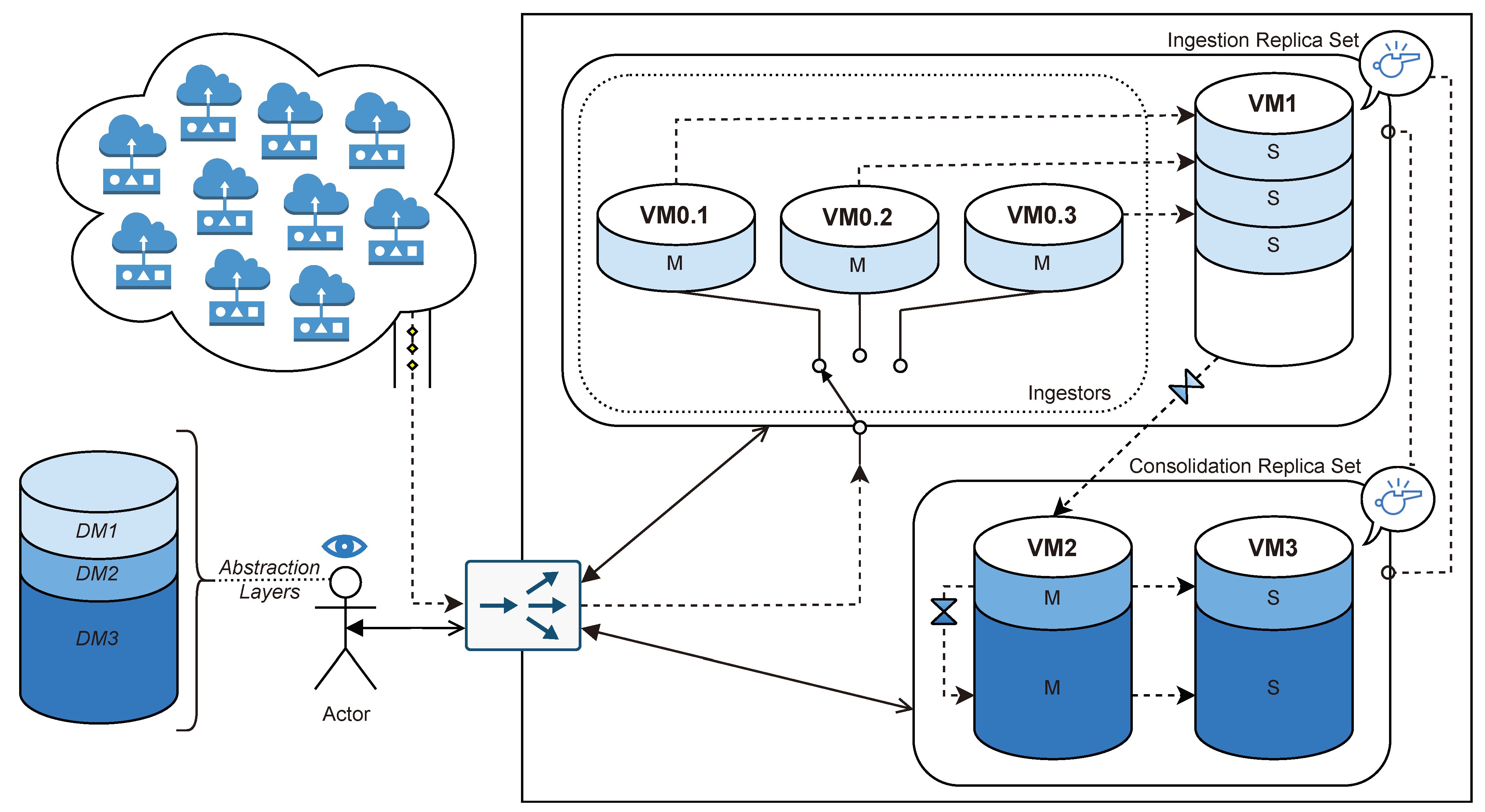
For instance, Figure 10 illustrates a distributed database under a sample Cascading Polyglot Persistence of three different data models following the approach explained in Section 4.

The distributed database is composed of two replica sets: the Ingestion Replica Set, holding Data Model 1, and the Consolidation Replica Set, holding both DM2 and DM3.

On the one hand, the sample Ingestion Replica Set is composed of four machines: Three of them hold a primary (or master) instance, whereas the last one holds all secondary instances in a vertical scalability fashion. The master nodes are expected to use an SSD device up to 600 MB/s, whereas the last node is expected to use a over-performing SSD device, up to 3500 MB/s, as it holds more shards. When cascading data from the Ingestion Replica Set to the Consolidation Replica Set, the secondary instances are used to avoid adding further workload to the primary ones while at the same time benefiting from data locality, as it is all stored in the same machine.

On the other hand, the Consolidation Replica Set is composed of two machines acting as a traditional replica set and based on large-storage HDD devices. This is due to the fact that the Consolidation Replica Set is expected to store big amounts of data, which is far more affordable in HDD devices. In addition, HDD devices are sufficiently efficient when performing sequential operations, such as historical querying [12].

When cascading data from DM2 to DM3, the primary node is used instead of the secondary one. This is due to the fact that ingestion instances must be primary ones. It would be possible to cascade data from the secondary node (VM3’s DM2) to the primary node (VM2’s DM3), which is, in fact, the pattern that the cascade from DM1 to DM2 follows. However, as DM2 and DM3 are stored in the same machine, the operation from primary to primary is far more efficient, as it avoids network and latency overheads.

Last, to assure an odd number of voters, each replica set is able to vote in the election of the other replica set through its respective secondary machines. This is represented by a whistle symbol.

The monitoring infrastructure composed of sensors ships data to the primary nodes of the Ingestion Replica Set through the router, whereas the user is able to query data regardless of the replica set in which data are stored. Moreover, thanks to the Polyglot Abstraction Layers implemented in the Cascading Polyglot Persistence approach, the user is able to see the whole system as a single instance and a single data model.

Thanks to this approach, the distributed database is able to maximize its ingestion performance, as time series databases for monitoring infrastructures are mostly targeted with write operations [24] while enabling fast data retrieval.

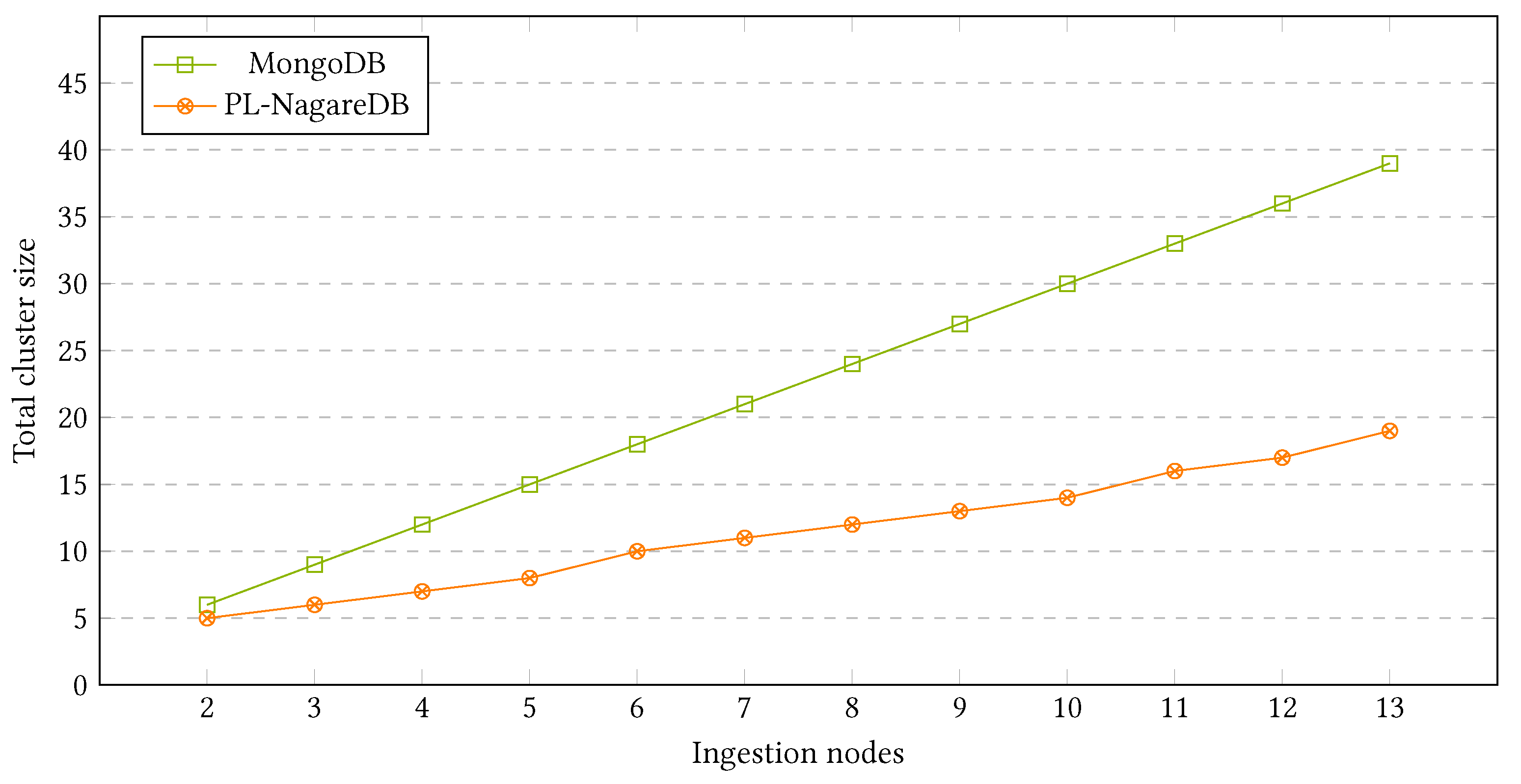
In addition, as seen in Figure 11, the cluster is able to substantially reduce its resource usage in terms of machines with respect to the total number of machines involved in ingestion operations. This is, in fact, one of the main objectives of this approach, as it is not intended to provide just a better performance but a reduced resource consumption as well. As explained in Section 4, this is achieved thanks to specialization, as each part of the database can grow independently. In the opposite scenario, when implementing more traditional approaches, the database acts and scales as a whole.

6. Experimental Setup

The experimental setup is intended to enable the evaluation of the performance of our approach in moderate-demand use cases. This is due to the fact that both Cascading Polyglot Persistence and the scalability approach presented in this research are intended for resource-saving scenarios, aiming at providing fast performance while minimizing resource usage. More precisely, this approach is implemented on top of NagareDB, a resource-efficient database [3], under Cascading Polyglot Persistence, as explained in Section 3.

Regarding the precise evaluated scenarios, the setup will consist of the architecture represented in Figure 10, from one to three ingestion nodes. Moreover, the experimental setup is only focused to enable the performance evaluation of the Ingestion Replica Set with respect to ingestion and multi-shard querying, as the Consolidation Replica Set and single-instance querying are not affected by this approach, delivering equal results as in previous benchmarks [14].

6.1. Cluster Infrastructure

The cluster is divided into two different parts: the Ingestion Replica Set and the Consolidation Replica Set. Each machine has its own specific hardware configuration and is able to communicate with any other machine through an internal network.

Moreover, as explained in Section 4.1, the machines will be set up for minimum resource usage to demonstrate that good results can be achieved with commodity machines if applying optimized techniques, such as the one presented here. More precisely, regarding the Ingestion Replica Set, hosting each shard will imply adding 1 further Gigabyte of RAM and 1 vCPU to the host machine that will have by default Ubuntu 18.04’s recommended minimum requirements [25], for instance:

• OS Ubuntu 18.04 LTS (Bionic Beaver)
• 2 GHz dual core processor or better
• 2 GB system memory

Regarding the Ingestion Replica Set hardware, there will be one machine per primary shard with the following configuration:

• OS Ubuntu 18.04 LTS (Bionic Beaver)
• 3 vCPUs @ 2.2Ghz (Intel® Xeon® Silver 4114)
• 3GB RAM DDR4 2666MHz (Samsung)
• 60GB - fixed size (Samsung 860 EVO SSD @ 550MB/s)

Regarding its secondary shards, there will be one machine for them all with the following configuration:

• OS Ubuntu 18.04 LTS (Bionic Beaver)
• (2 + #holdedShards) vCPUs @ 2.2Ghz (Intel® Xeon® Silver 4114)
• (2 + #holdedShards) GB RAM DDR4 2666MHz (Samsung)
• (60GB ∗ #holdedShards) - fixed size (Samsung 970 SSD NVMe @ 3500MB/s)

For instance, when the infrastructure consists in three ingestion nodes, this vertical scalable machine will be assigned with:

• OS Ubuntu 18.04 LTS (Bionic Beaver)
• 5 vCPUs @ 2.2Ghz (Intel® Xeon® Silver 4114)
• 5 GB RAM DDR4 2666MHz (Samsung)
• 180GB - fixed size (Samsung 970 SSD NVMe @ 3500MB/s)

The presence of the Consolidation Replica Set in this evaluation is just a testimonial approximation as explained above. It is deployed over HDD devices and using Ubuntu’s minimum requirements with respect to the number of CPUs and gigabytes of RAM.

6.2. Data Set

The dataset used during the evaluation of this approach is generated by a simulated monitoring infrastructure. This simulation is set up following real-world industrial settings, such as the ones of our external collaborators. More precisely, the simulated monitoring infrastructure is composed of 500 different sensors, where a sensor performs a reading every minute. Sensor readings (R) follow the trend of a normal distribution with mean $\mu$ and standard deviation $\sigma$:

$$R\sim \mathcal{N}(\mu ,{\sigma }^2):\mu \sim \mathcal{U}(200,400),\sigma \sim \mathcal{U}(50,70)$$

(1)

where each sensor’s $\mu$ and $\sigma$ are uniformly distributed.

The simulation is run until obtaining a 10-year historical period from 2000 until 2009 included, so the total amount of triples is 2,630,160,000.

7. Analysis and Evaluation

This section is intended to analyze and evaluate the performance of the proposed approach, not only by showing its raw metrics, but also by providing techniques from which database architects can diagnose efficiency leakages and further improve the approach performance, tailoring it to each specific use case.

As explained in Section 6, this section analyzes and evaluates the performance from one to three ingestion nodes, focusing on the Ingestion Replica Set, both in ingestion operations and multi-shard queries.

7.1. Ingestion Capabilities

The ingestion will be evaluated in two different shipping scenarios. In the first one, data are shipped to be ingested just when being generated, in a real-time fashion. On the second one, the shipper will accumulate a certain amount of sensor readings to ship them in a near-real-time fashion. The ingestion is evaluated under a simulation using the data explained in Section 6.2. However, in these experiments, the nature of data loses certain importance, as the experiment will be sped up, not waiting to ship data each minute as would happen in a real scenario. This method intends to provide a realistic maximum ingestion performance of each approach. More precisely, it is performed simulating a synchronized and distributed scenario. Each data shipper will only consider that an ingestion operation is finished when: (1) the database acknowledges the data reception, and (2) the database persists its write-ahead log, which ensures durable write operations. When a write operation is finished, the shipper will execute the following one in a sequential pattern. Thus, the faster the database is able to receive and safeguard the data, the faster that each shipper will send the following data triplet, being able to process the dataset more speedily. Consequently, the streaming rate and its ingestion speed are inherently adjusted by the database according to its performance offer. The metric used to evaluate the ingestion performance is the average triplets writes/second, where each triplet, as explained in Section 2.6, is composed of a time stamp, sensor ID, and value.

7.1.1. Real-Time Ingestion

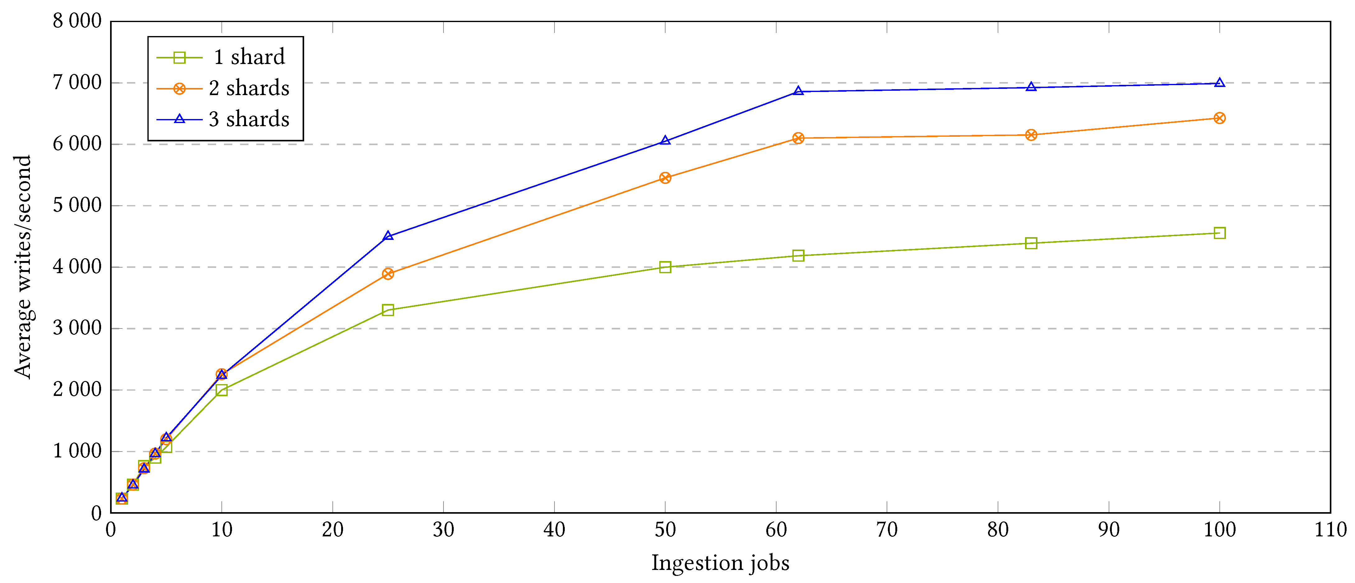
This section evaluates the ingestion ability and performance of the cluster under a strict real-time simulated monitoring infrastructure. Thus, data are shipped individually in a triplet structure as soon as it is generated. The evaluation is carried out from one to three ingestion shards and from 1 to 100 shipping or ingestion jobs. Each shipping job will be shipping an equal amount of data, dividing the total triplets among them. For instance, if the setup is composed of 10 shipping jobs, each one will be in charge of shipping and ensuring the correct ingestion of the data from 50 sensors, as the total amount of sensors is 500. Thus, the more shipping jobs, the more parallelism can be achieved, as the system receives more simultaneous workload. Last, when adding ingestion shards or nodes, the ingestion can be further parallelized as several nodes can collaboratively handle the workload coming from the shipping jobs.

As seen in Figure 12, adding further shards to the ingestion cluster is able to generally provide an increased speedup in data ingestion in terms of writes/second. However, the plot shows some interesting insights:

• Until reaching 10 simultaneous jobs, the performance of the cluster with one, two, or three ingestion shards remains virtually equal. This is due to the fact that a single machine is able to handle the ingestion parallelism achieved with less than 10 simultaneous jobs, which implies that in that configuration there is no benefit in adding more resources. Thus, it is important to evaluate the requirements of each scenario before the setup, as in this case, adding more ingestion resources only increases the costs and not the performance.
• In scenarios with approximately 20 or more parallel ingestion jobs, adding more ingestion resources implies a better ingestion speed. In addition, the difference between 3 and 2 shards is approximately 50% of the difference between 1 and 2, which makes proportional sense. However, the speedup is far from the perfect scaling, providing better but not cost-efficient results.
• Any of the cluster configurations from one to three shards did not reach the parallel slowdown point—when adding further parallel jobs reduces the system’s performance. However, it is noticeable that starting from approximately 80 parallel jobs, the ingestion reaches almost a speedup stagnation point—when adding further parallel jobs implies a poor or nonexistent performance gain.

We conclude that when following real-time ingestion, adding more machines can actually speed up the system, but not efficiently. This can be explained due to the extremely high granular approach, where each sensor reading is shipped individually along with its corresponding metadata. This implies that the messages/second are really high, but the megabytes/second writing of real data are pretty low. Consequently, the router has to constantly ship individual messages to the right shard, the network has to handle a huge amount of independent messages, and the shipper CPUs have to be constantly sending data and waiting for their acknowledgement, spending CPU cycles. This ends up causing a big overhead to the whole system, wasting resources, and limiting the scalability of the application [26].

This is the main reason why even most sophisticated real-time systems are not truly real real-time systems, but actually near real-time systems [27].

7.1.2. Near Real-Time Ingestion

Near real-time ingestion does not intend to ingest data as soon as it is generated, but to accumulate it up to a certain moment, aiming at a real-time enough solution. It is a technique implement by some of the most relevant streaming platforms to ensure efficiency [28,29]. This accumulated data, typically called micro-batches, are ingested close to the moment where they were generated, but not immediately. Consequently, as data are sent in groups, the global overhead of the system is reduced, and the performance can be generally increased. Thus, the bigger the micro-batch, the more efficiently it will be ingested; however, the more it accumulates before shipping, the less real-time it will be. Finding the best balance between these two components is use-case specific, meaning that there is no standard configuration and that to maximize the performance, this will have to be evaluated in each scenario.

To provide some steps or guideline when looking for the best performance according to the use-case real-time needs, this research utilises the following notation according to the data organization explained in Section 2.6:

$$CL:\#R\ast RL$$

(2)

where CL is the column length, #R, the number of rows, and RL, the size of the individual rows, taking into account that:

$$\#R\ast RL=\#S$$

(3)

where #S is the total number of sensors.

For instance, the dataset grouping represented in Figure 13, where each group has a row size of 10 and a column length of 2, is represented as:

$$2:50\ast 10$$

(4)

where 500 (50 × 10) is the total number of data sources or sensors, making each group to be composed of 20 sensor readings.

The setups to be tested are represented in

Table 2. The different operations to be performed and their identification as a combination of the row size and the simultaneous jobs.

Operation ID	Simultaneous Jobs	Row Size
NCOL:1 × 500	1	500
NCOL:5 × 100	5	100
NCOL:10 × 50	10	50
NCOL:25 × 20	25	20
NCOL:50 × 10	50	10

, where the NCOLS parameter will be 2, 10, and 50, from more real-time to less, as the columns represent the temporal dimension, or the time steps. The methodology will follow a local maximum approach. The best configurations for NCOLS = 2 will be evaluated and analyzed for NCOLS = 10, repeating the process for NCOLS = 10 and NCOLS = 50.

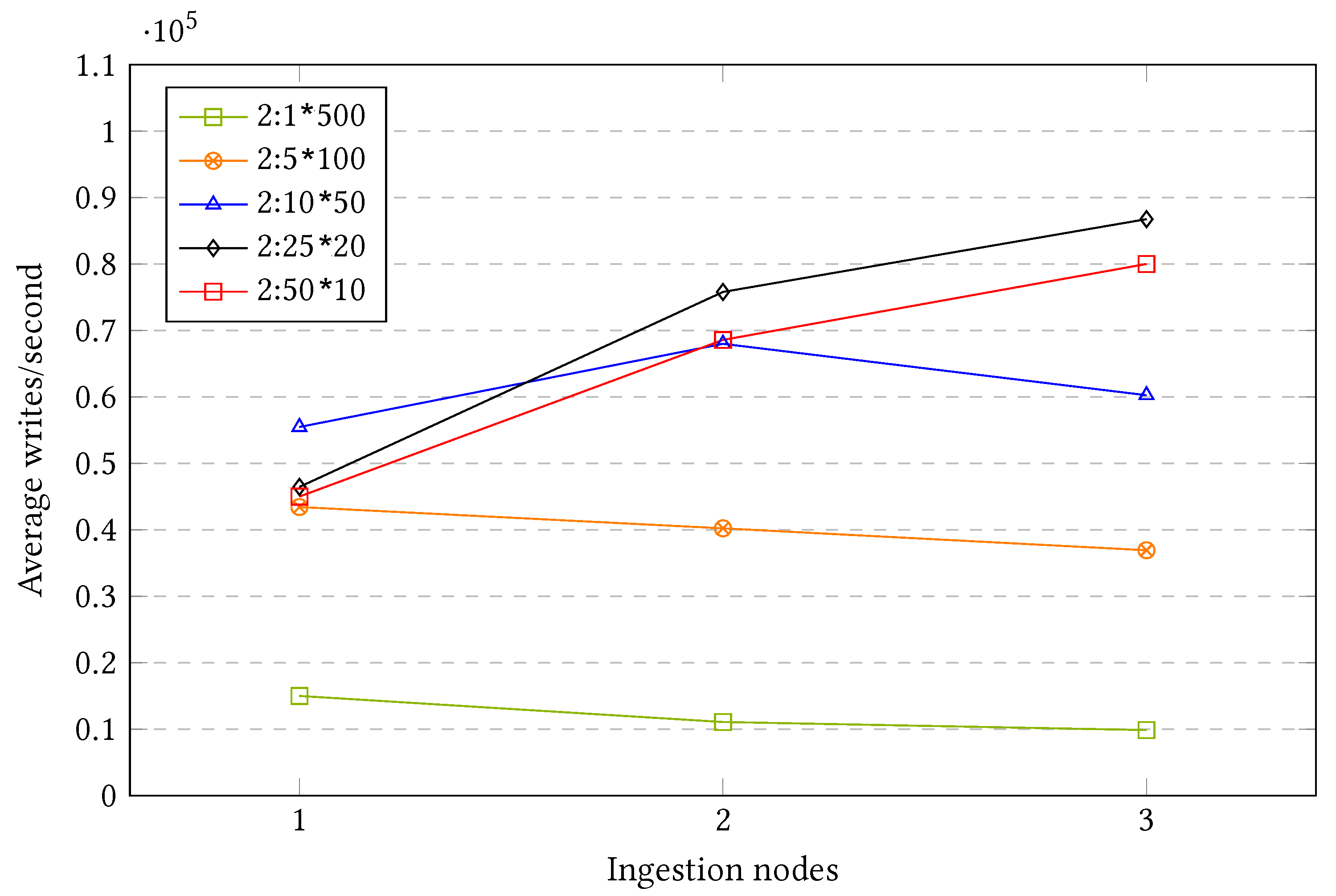
7.1.3. Micro-Batching: 2 Time Steps

With a column depth of two time steps, the shipper will send the data with a single time stamp difference, meaning that it does not ship data once it gathers one reading but when it gathers two. It is the closest approximation to real real-time ingestion.

Figure 14 shows the results after executing the different setups with one, two, and three ingestion nodes or shards.

As seen in the above figure, the performance speedup according to the number of ingestion nodes greatly differs depending on the row group configuration. Some of the most interesting insights that the plot provides are:

• When using one single group, a row of size 500 (2:1 × 500), the performance is the lowest in comparison to the other ingestion alternatives. In addition, when adding further ingestion nodes or shards, instead of increasing, the performance decreases. This shows that adding further resources does not always improve the system performance, at least if the approach is not evaluated holistically.
• When dividing all the sensors in five different groups and shipping them in parallel (2:5 × 100), the performance improves greatly in comparison to the previous group. However, it suffers from the same issue: Adding further resources decreases the system performance.
• The third, intermediate, configuration (2:10 × 50) is able to offer some speedup when scaling out; however, this only applies when adding a second machine. Thus, when adding a third machine, the system worsens its performance, remaining better than with a single ingestion shard but worse than with two machines.
• The TOP two most granular groups (2:25 × 10 and 2:50 × 10) offer the best scalability among all the options with a column size of two. However, the most scalable option is not the most granular one but the second: 2:25 × 20.
• Although the two most granular setups offer the best scalability, the intermediate option (2:10 × 50) is the most efficient one if there is only one ingestion machine available, such as in a monolithic approach.

In addition, there is a relevant pattern that keeps repeating across the different setups. The speedup sometimes ends up decreasing when adding more shards, which seems contrary to the objective of scalability. Particularly, the two less granular setups constantly decrease their performance when scaling out, and the intermediate configuration increases its performance when adding a second node, while later decreasing its performance when adding a third one.

This phenomenon is caused by two relevant events that can occur when performing bulk ingestions over distributed databases: Multi-Target Operations, and Parallel Barriers.

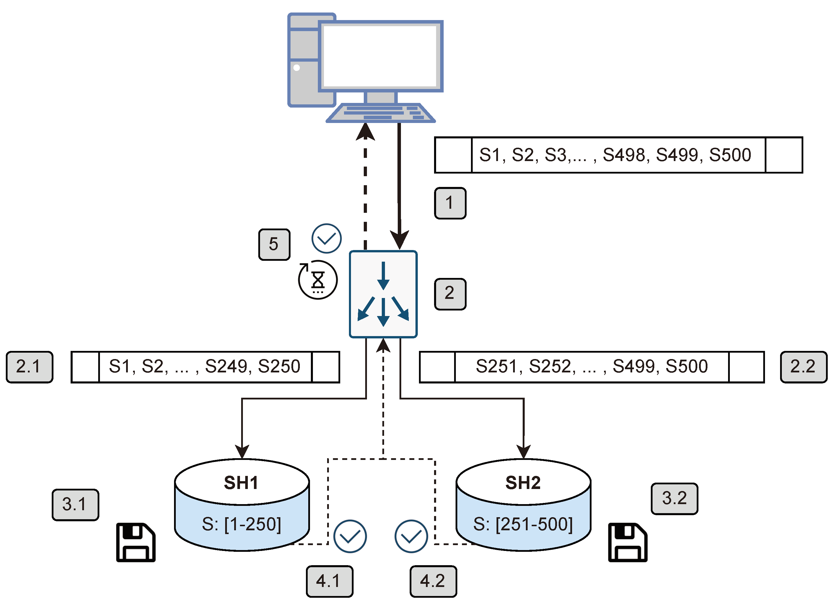
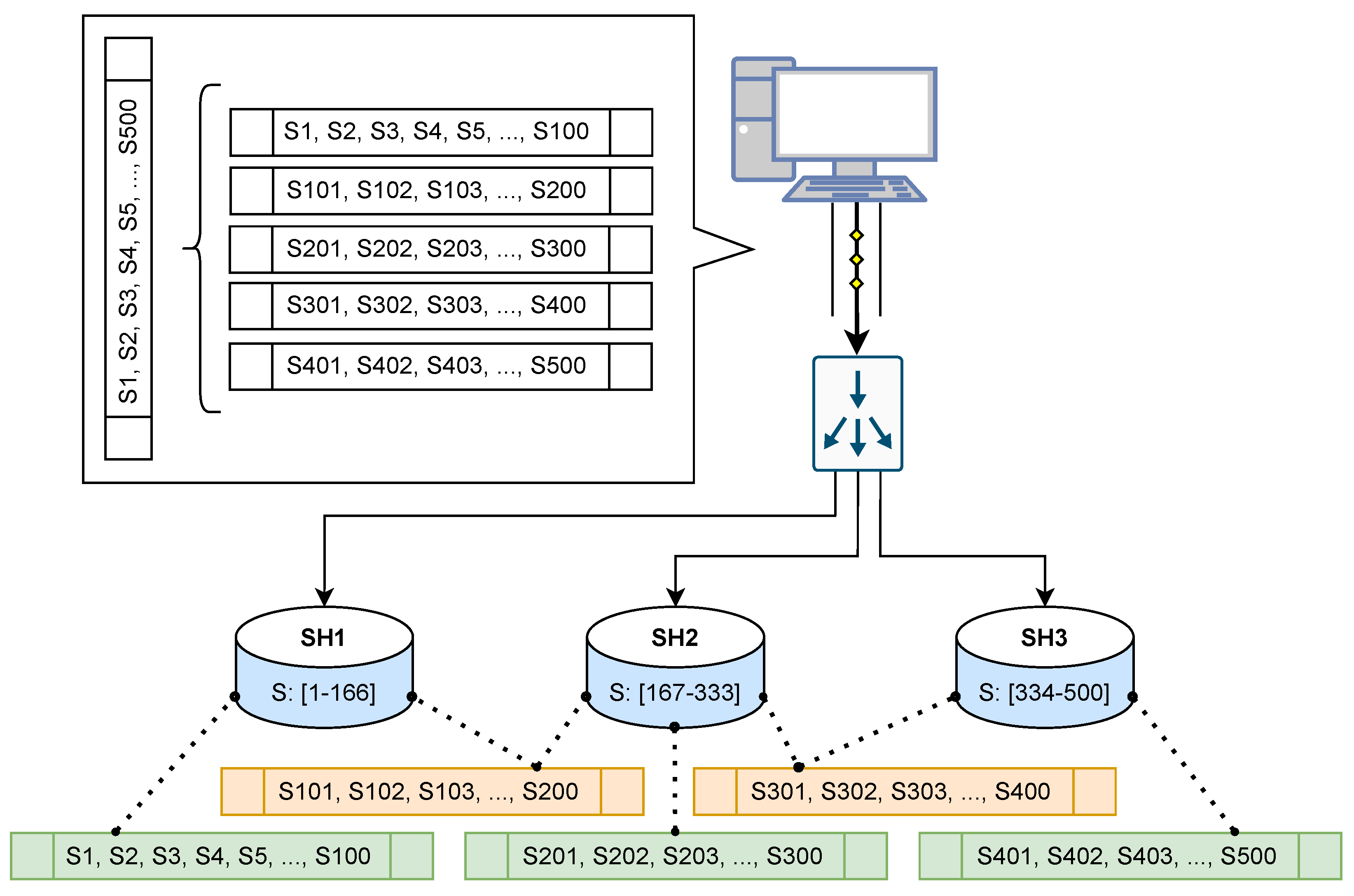
Figure 15 is composed of 5 different main steps that represent a brief data ingestion procedure under a 1:1 × 500 setup with two ingestion shards:

• The shipping machine intends to ship a group of 500 triplets that contains the sensor readings and its metadata, from S1 to S500.
• The router receives the data and intends to redirect it to the appropriate shards for their ingestion. However, as there are two shards, each one is in charge of holding half of the data. This means that the router will have to perform a Multi-target operation, meaning that it will have to split the group, a fact that produces a system overhead, and to perform two different ingestion operations, each targeting a different shard: 2.1, and 2.2.
• Each shard receives its respective operation (3.1 and 3.2) and persists its data to the disk or write-ahead log, keeping it safe.
• Once each operation has been completed, each shard returns an acknowledgment (4.1 and 4.2), given that the ingestion operations are synchronous.
• However, as the operation was initially just one although it was split in two different sub-operations, it is not possible to consider the operation finished until all sub-operations have also been completed. This phenomenon is especially relevant when using heterogeneous hardware in the cluster. It is actually a Parallel Barrier, which means that the total operation time will depend on the slowest sub-operation time, reducing the system performance if both shards do not spend exactly the same time per operation. Once both sub-operations are completed, the shipper receives the acknowledgement of the successfully finished operation and is able to continue with its remaining ones.

This phenomenon occurs in the previously selected configurations and leads to a penalization when adding more machines. Thus, if the system was able to handle the requested workload without that newly-introduced machine, and in addition, we introduce the unequal load balance penalization, the system’s performance drops. Thus, it is important to take into account this phenomenon when designing a distributed database and act accordingly to reduce its occurrences and negative effects.

In the scenario of Figure 16, the 500 sensors are divided across three different shards. When the shipper intends to send 5 groups of 100 sensors each, some groups can be directly shipped to a shard, whereas other groups will have to be split. For example, S1–S100 group can be directly routed to Shard 1 that holds S1–S166 data, but group S101–S200 will have to be split, into a Multi-Target Operation to SH1 (S1–S166) and SH2 (S167–S333). Thus, some operations will finish speedily, whereas the split operations will be slower due to the Multi-target Operation.

Last, regarding the intermediate configuration (2:10 × 50) as seen in Figure 14, a mountain-shaped performance is achieved: A second shard introduces further performance, whereas a third one decreases it. This is, in fact, also explained by Multi-Target Operations and Parallel Barriers.

When dividing the 10 groups into two shards, each shard receives 5 groups, meaning that there are no Multi-Target Operations, nor a Parallel Barrier caused by a group split. However, when adding a third shard, the fourth group is split across the first and second shard, and the seventh groups is split across the second and third shard, which causes the performance drop phenomenon explained previously.

Thus, when configuring a distributed database following the approach presented here, it will be important to detect, reduce, or avoid this problems, selecting configurations that fit both the dataset and the architecture.

7.1.4. Micro-Batching: 10 Time Steps

Taking into account the methodology explained in this section, the following configurations are selected to be evaluated:

• 10:10 × 50
• 10:25 × 20
• 10:50 × 10

as these row sizes were the most performing ones in the previous evaluation.

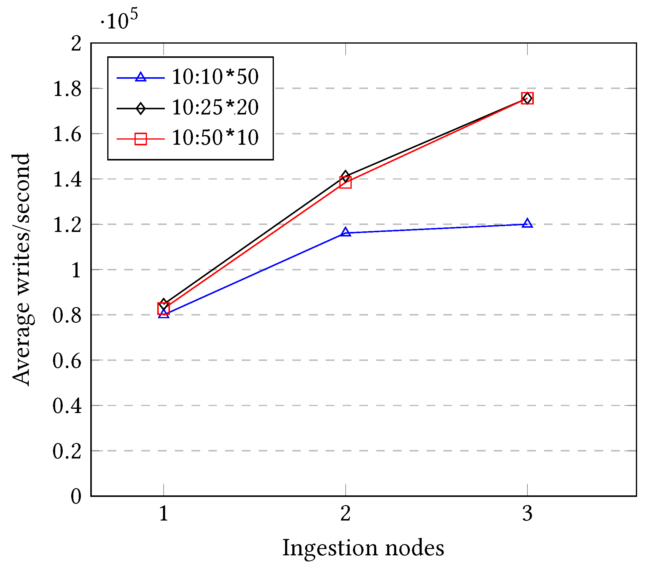
As seen in Figure 17 in comparison to Figure 14, the overall performance is far better with a column length of 10 than with a column length of 2. For instance, the three different three setups when using a column length of 2 under one single node write approximately 50,000 triplets/second, as seen in Figure 14, whereas when using a column length of 10, the same setup reaches 80,000 writes/second. Consequently, this extension in the micro-batching size trades distance for real time with cost-efficiency.

In addition, some of the most interesting insights that the plot provides are:

• The setup that involves less groups, 10:10 × 50, is the less scalable one. It is able to scale with certain speedup when adding a second machine, but when adding a third one, it virtually provides the same performance. This is due to the Multi-Target Operations and the parallel barrier that do not take place under that configuration with two shards, but it appears when adding a third one.
• All three setups virtually provide the same performance if one single shard is used, which probably means that 80,000 triplet writes/second in the maximum speed that the used hardware is able to provide when using one ingestion node.
• The top two most granular setups (10:50 × 10 and 10:25 × 20) provide an equivalent performance and a virtually equal scaling speedup in all different configurations from 1 ingestion node until 3 ingestion nodes. Their write performance reaches approximately 180,000 triplet writes/second.

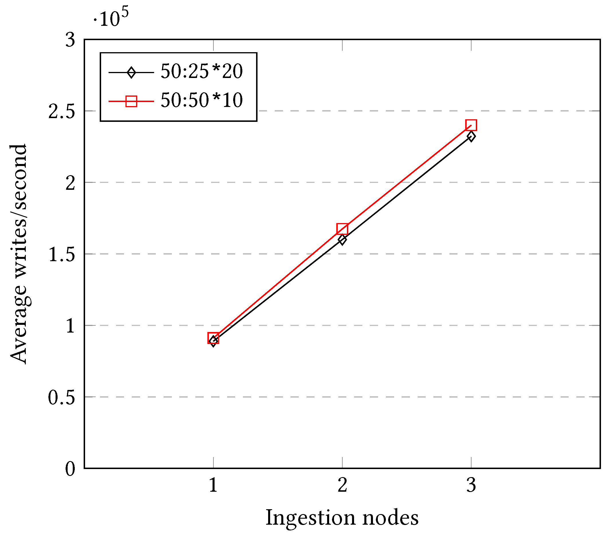
7.1.5. Micro-Batching: 50 Time Steps

After selecting the two most performing setups in the previous micro-batching approach and repeating the experiments with a column size of 50 time steps, the experiments yield the following results:

As can be seen in Figure 18, both approaches reach an almost perfect scalability performance, and a maximum speed of almost 250,000 triplet writes/second when using three ingestion nodes. It is important to take into account that under a setup of three ingestion nodes the ingestion still suffers from the problems explained previously regarding Multi-Target Operations and Parallel Barriers. However, as the parallelization is maximized, creating a big number of simultaneous short-lasting jobs, the negative effects are diluted, making them not that relevant in this setup. Thus, each scenario using the approach presented in this research is invited to evaluate and tune the parameters of the setup to reach the desired balance between scalability performance and real-time ingestion, but targeting to an outcome similar to the one of Figure 18.

7.2. Querying Capabilities

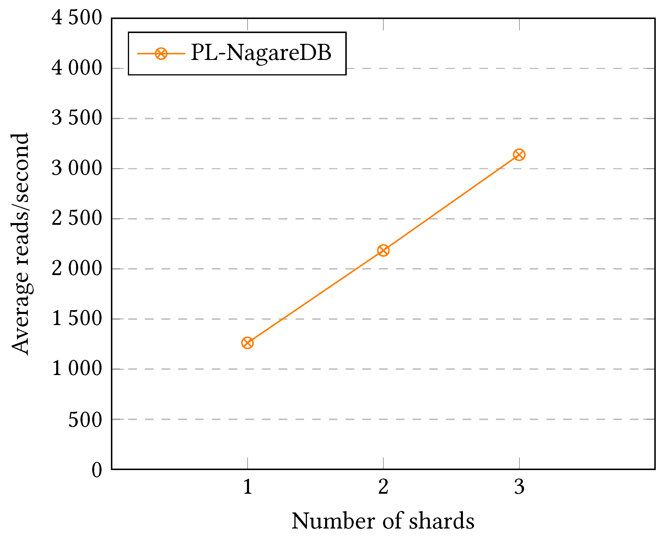
To evaluate the scalability performance of the Ingestion Replica Set, this evaluation is run with the different cluster configurations from one to three ingestion shards. In addition, we define a high parallelizable query so that a query can be answered using all the available hardware.

The query itself belongs to the category of time-stamped querying [14]. These queries are intended to obtain all sensor readings for a specific time stamp. As sensor readings are divided across all the different shards when performing a time stamped querying, all nodes will be asked to work collaboratively, which allows us to evaluate the scalability performance.

After evaluating the query against 10 different random time stamps, cleaning the cache after each execution, the result was as follows:

As can be seen in Figure 19, the scalability performance achieved is outstanding. This is due to the fact that it does not involve a big amount of parallel petitions that might overwhelm the system as real-time ingestion does. In this case, the query is answered by 1, 2, or 3 nodes that are able to efficiently divide the workload among them.

8. Conclusions

We introduced and discussed the concepts and obstacles that organizations have to bear in mind when deploying infrastructures for distributed databases, not only in terms of software/hardware approaches and performance, but also in terms of resource expenses.

To alleviate those obstacles, specifically aiming at reducing infrastructure costs, we introduced a holistic approach for scaling time series databases under Cascading Polyglot Persistence, following a cluster fashion. This approach intends to be understood as a model or departure point for scenarios that target, on the one hand, enabling efficient data ingestion and retrieval and, on the other hand, reducing the number of needed machines.

More precisely, we set our starting point to be the Cascading Polyglot Persistence technique that aimed to enable cost-efficient time series data management but lacked a specific scalability approach, relying on generic ones.

When introducing our scalability approach, the database showed to fit better to the nature of Cascading Polyglot Persistence, improving its performance and maximizing its objectives. In particular, it was able to reach upstanding speedup performances, up to 85% improvement, in comparison to a theoretical and perfect scenario, when executing multi-shard operations. Moreover, it was able to greatly reduce the number of needed machines and obtained excellent results when using commodity machines with configuration requirements as low as just 3GB of RAM and 3 vCPUs.

More precisely, when deploying three low-requirement ingestion nodes under an internal network, the distributed database was able to reach a writing speed of almost 250,000 triplets/second, each composed of three different data types, while also ensuring data safety. Thus, our approach exemplifies that high performances can be achieved, while also ensuring data safety, not only by adding further expensive hardware, but also when using efficient software and tailored architectural approaches.

Last, our research illustrates how adding more machines in our time series data context does not always imply a positive performance speedup. This further contradicts the idea that increasing the system’s performance can be obtained by simply adding more resources. Thus, analyzing the interaction between the hardware and the software configurations, as exemplified in this research, becomes a mandatory step for efficient distributed time series databases.