
RSS-Based Wireless LAN Indoor Localization and Tracking Using Deep Architectures


Abstract
:1. Introduction
- Four different deep network architectures of MLP, CNNs, and LSTMs are proposed and their performance results are compared with one another and with the existing probabilistic-based approaches.
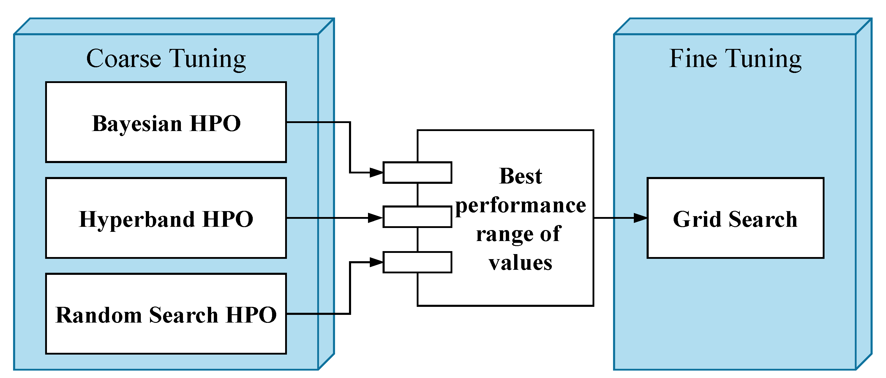
- Extensive experiments were carried out on real-world data to identify the optimum deep learning model parameters using proposed two-stage hyperparameter optimization (HPO) techniques (e.g., Bayesian Optimization, Hyperband, Random Search, and Grid Search).
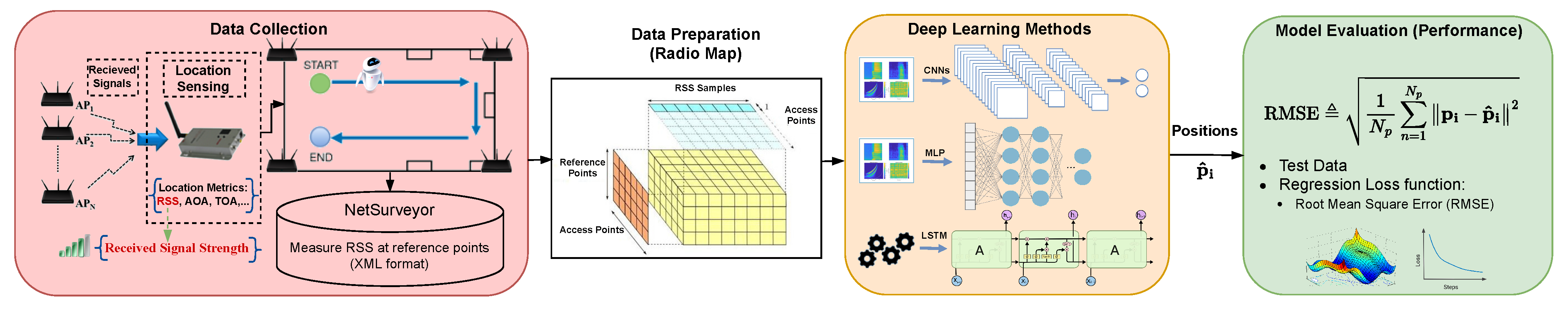
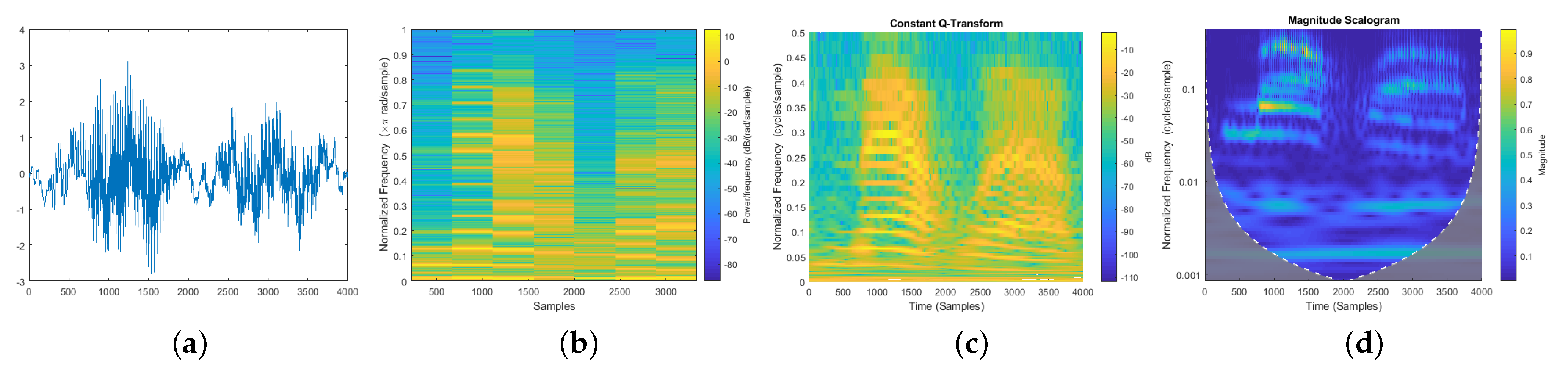
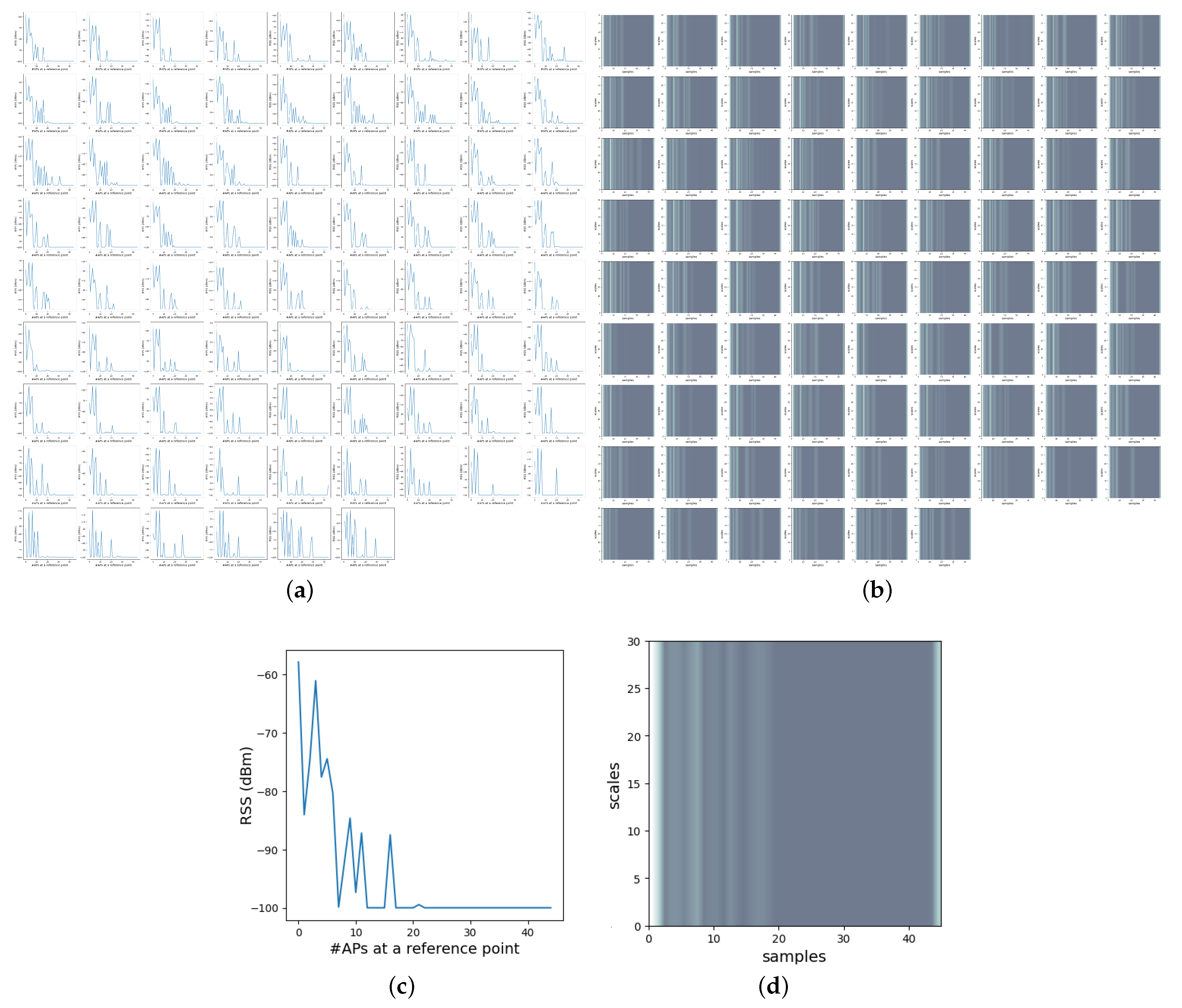
- A novel data set collected in the faculty building, consisting of two types of data in the form of stationary and walking data containing RSS measurements in XML format, was built. The collected RSS measurements were parsed and converted into a radio map, followed by the data preparation process. In order to eliminate the need for expertise in the field, the RSS image data set were obtained using Continuous Wavelet Transform (CWT) and also sequential data were generated to train the deep network models.
2. Related Work
3. Data
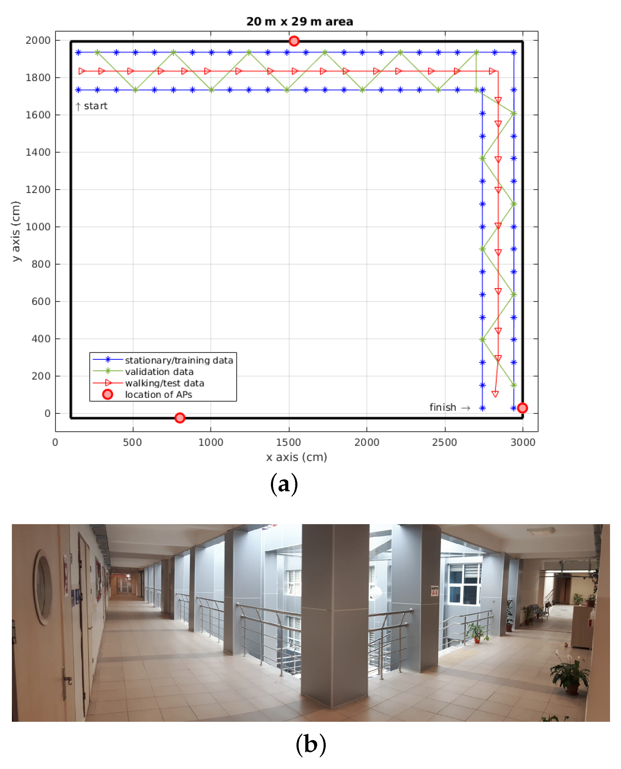
3.1. Data Collection
3.1.1. Training and validation data
3.1.2. Testing Data
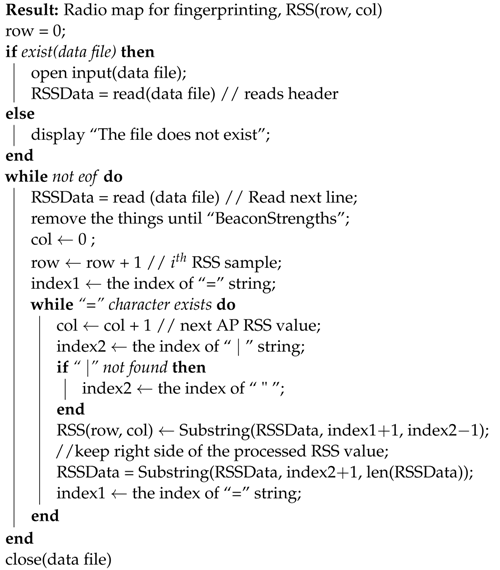
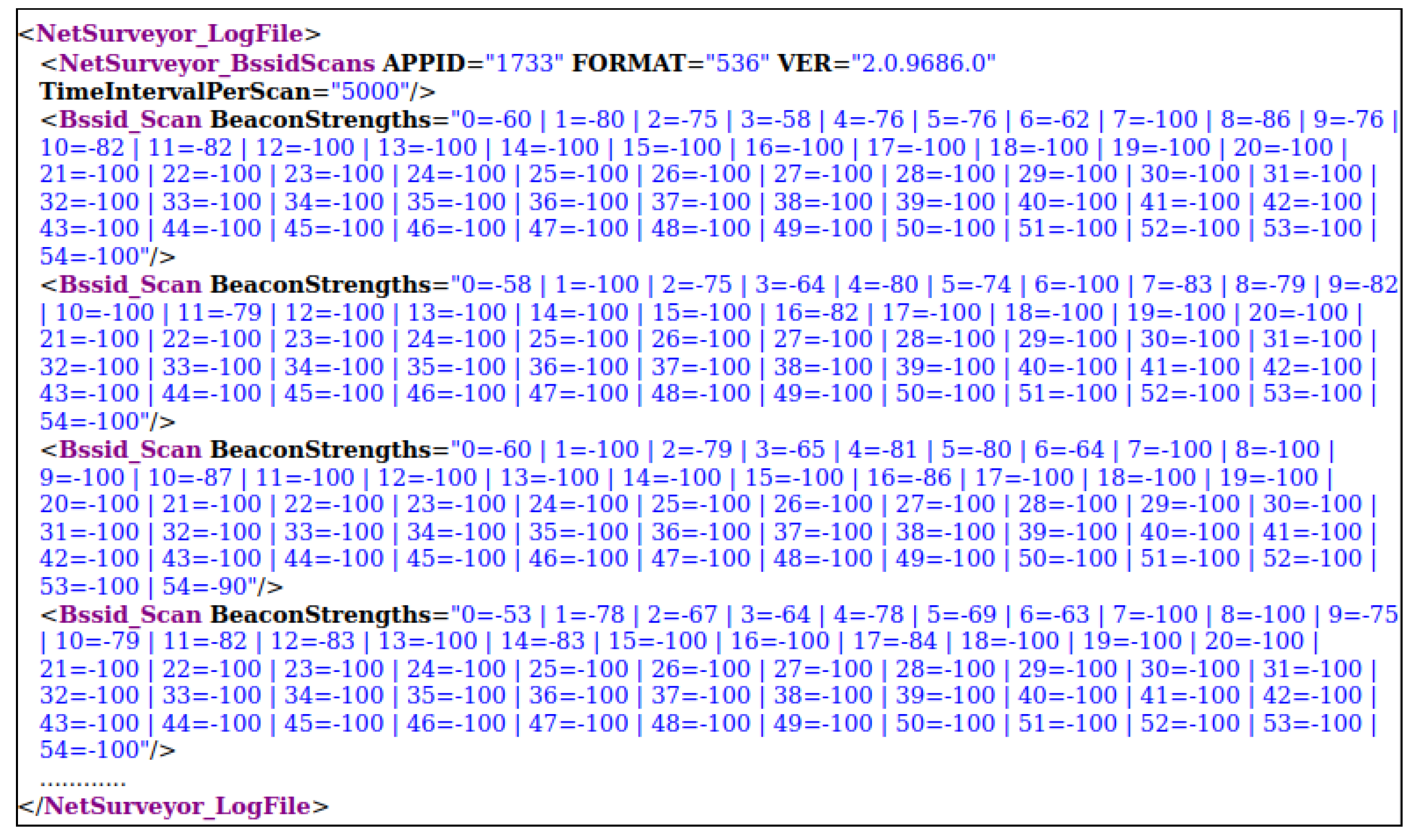
3.2. Preparing Data
| Algorithm 1: Data parsing method for the recorded XML data using Netsurveyor program. |
 |
- Removing and fixing outliers or inconsistencies caused by measurement errors of RSS data from APs. This was due to the natural variations in RSS data, it is likely to receive outlier data. A defined standard deviation from the mean was used to detect outliers assuming that the data had been coming from a Gaussian distribution. The outlier data was corrected with a time-average interpolation approach that was the mean of samples collected at each anchor point taken from each AP.
- In the event of no data reception at a particular AP, missing RSS values were filled in with a value of −100 dB as the neutral integer to ensure data integrity.
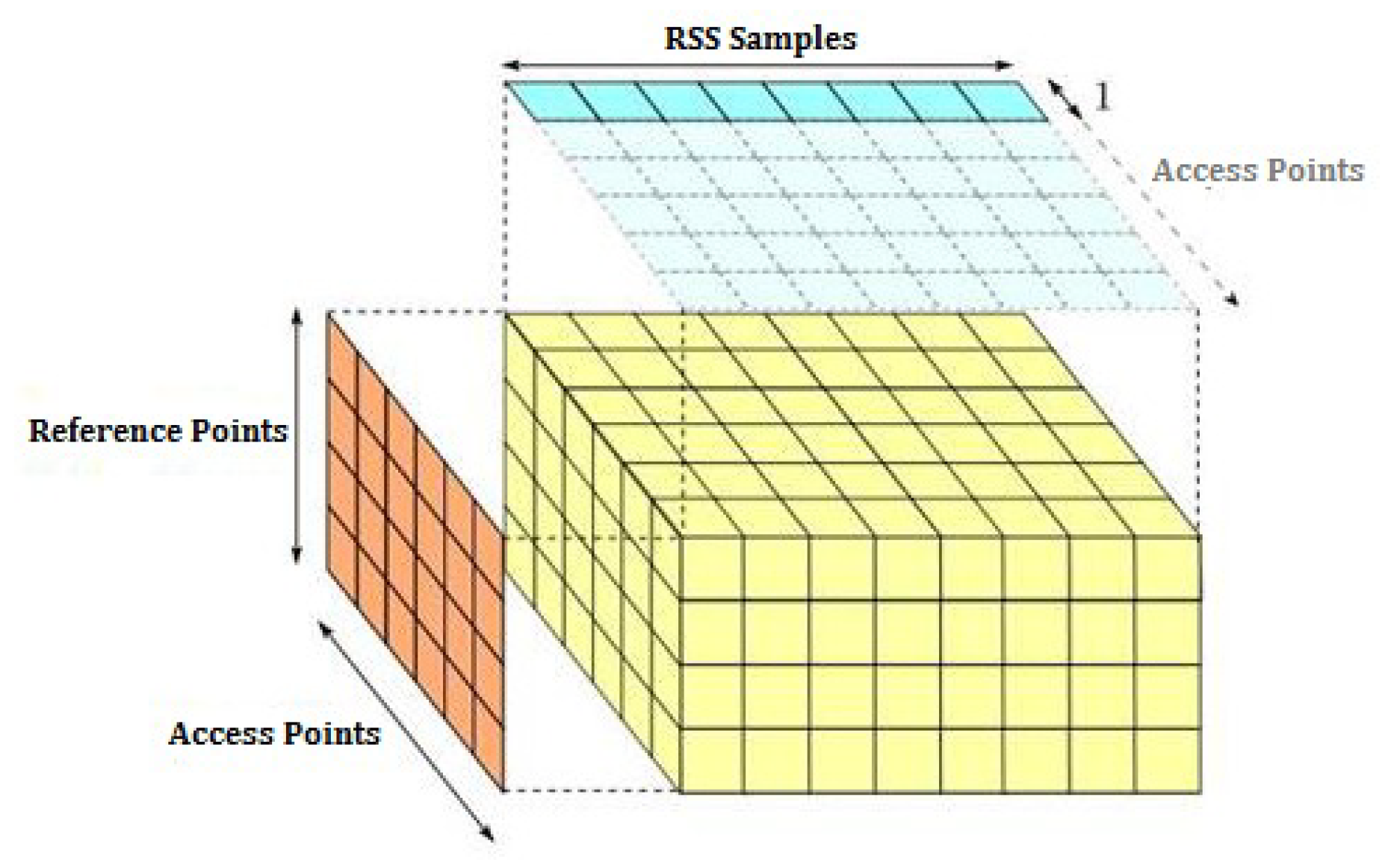
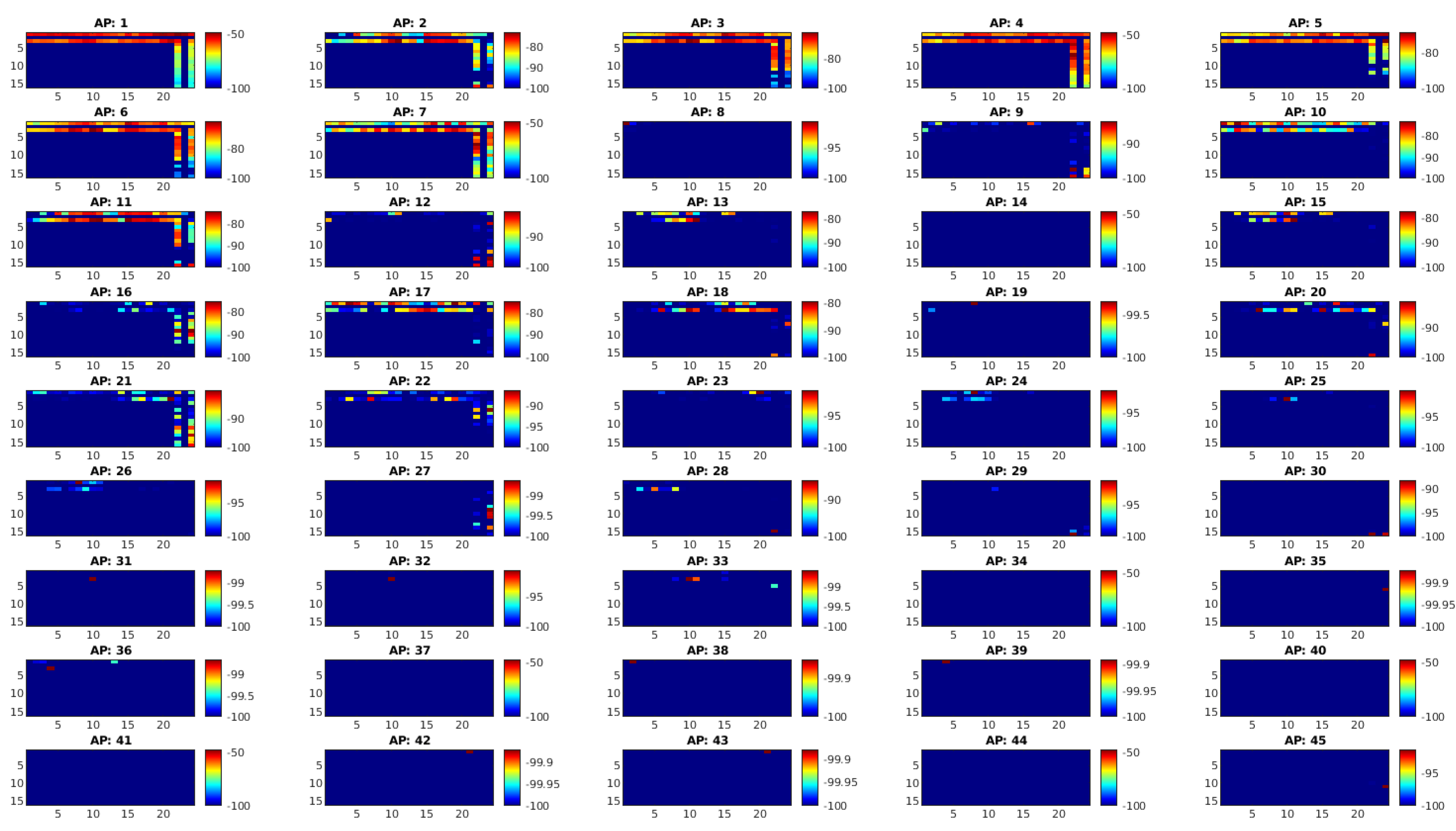
- As a result, a 3D radio map with the dimension of (samples per location, APs, reference points) was built and used in estimation algorithms as given in Figure 5.
4. Methods
- Obtaining image data set of RSS fingerprint matrices.
- Applying deep network models (i.e, MLP, 1D CNN, 2D CNN, LSTM) to predict the positions. Because we target the tracking problem, where the next location is highly dependent on the previous positions and the goal is to output a 2D spatial coordinate or position, WLAN positioning is formulated as a regression problem rather than a classification problem.
- Carrying out extensive experiments to determine the impact of various deep learning system components by the hyperparameter tuning process.
- Reporting the models’ performance. Positioning error is commonly evaluated as the euclidean distance between the actual position and its estimate. In this study, RMSE performance measure was used on training, validation, and test sets as shown in Equation (1). The RMSE measure was preferred since it penalized large errors and produces errors that were in the same unit as the prediction positions. The objective of the deep learning model was to minimize the RMSE loss function defined as the norm of difference in centimeters between all true positions () and estimated positions ().
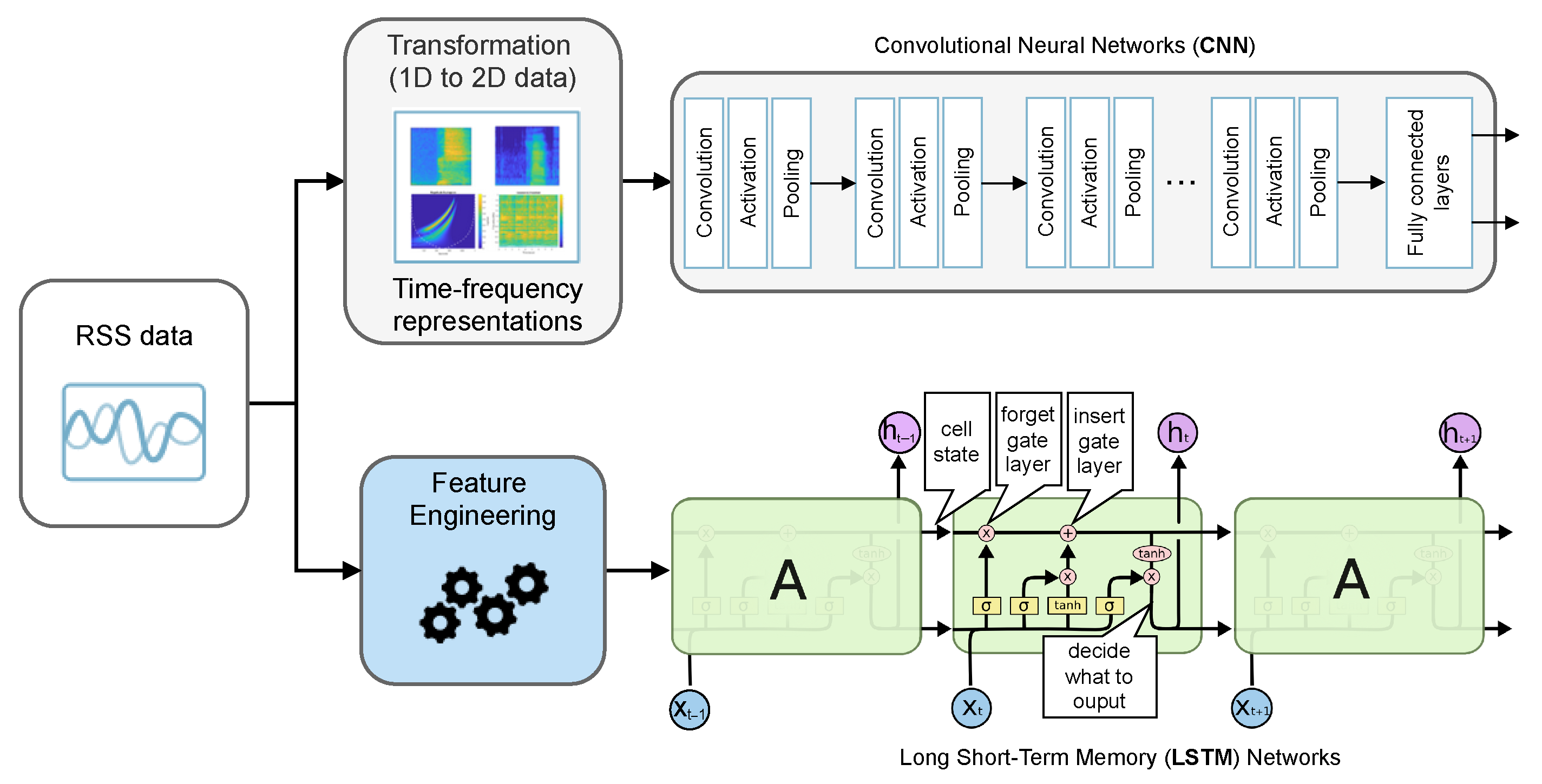
4.1. RSS Time-Frequency Transformations (RSS Image Data Set)
4.2. Multi-Layer Perceptron Neural Networks (MLPs)
4.3. Convolutional Neural Networks (CNNs)
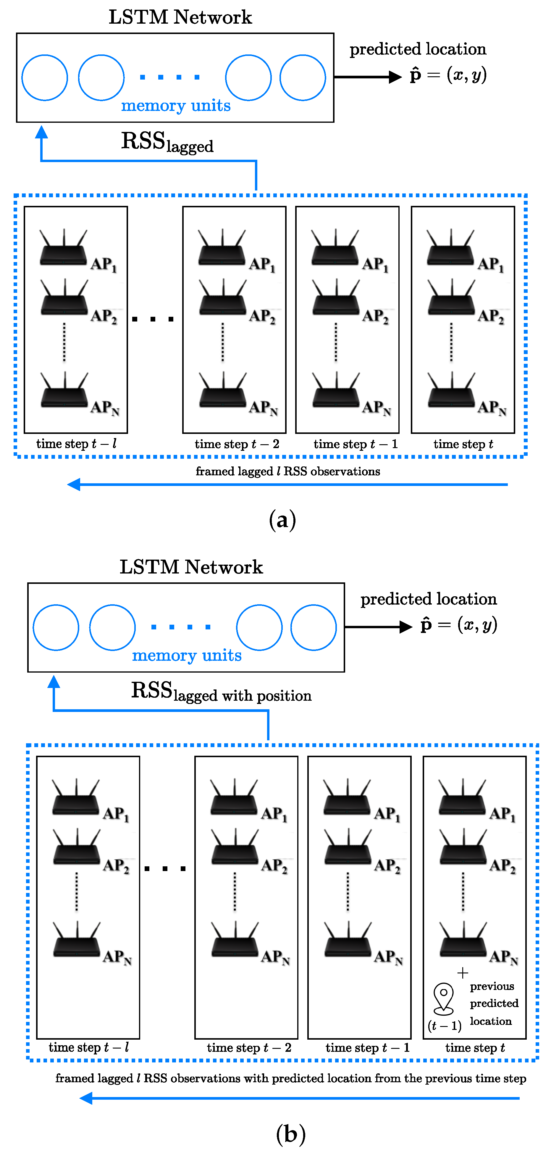
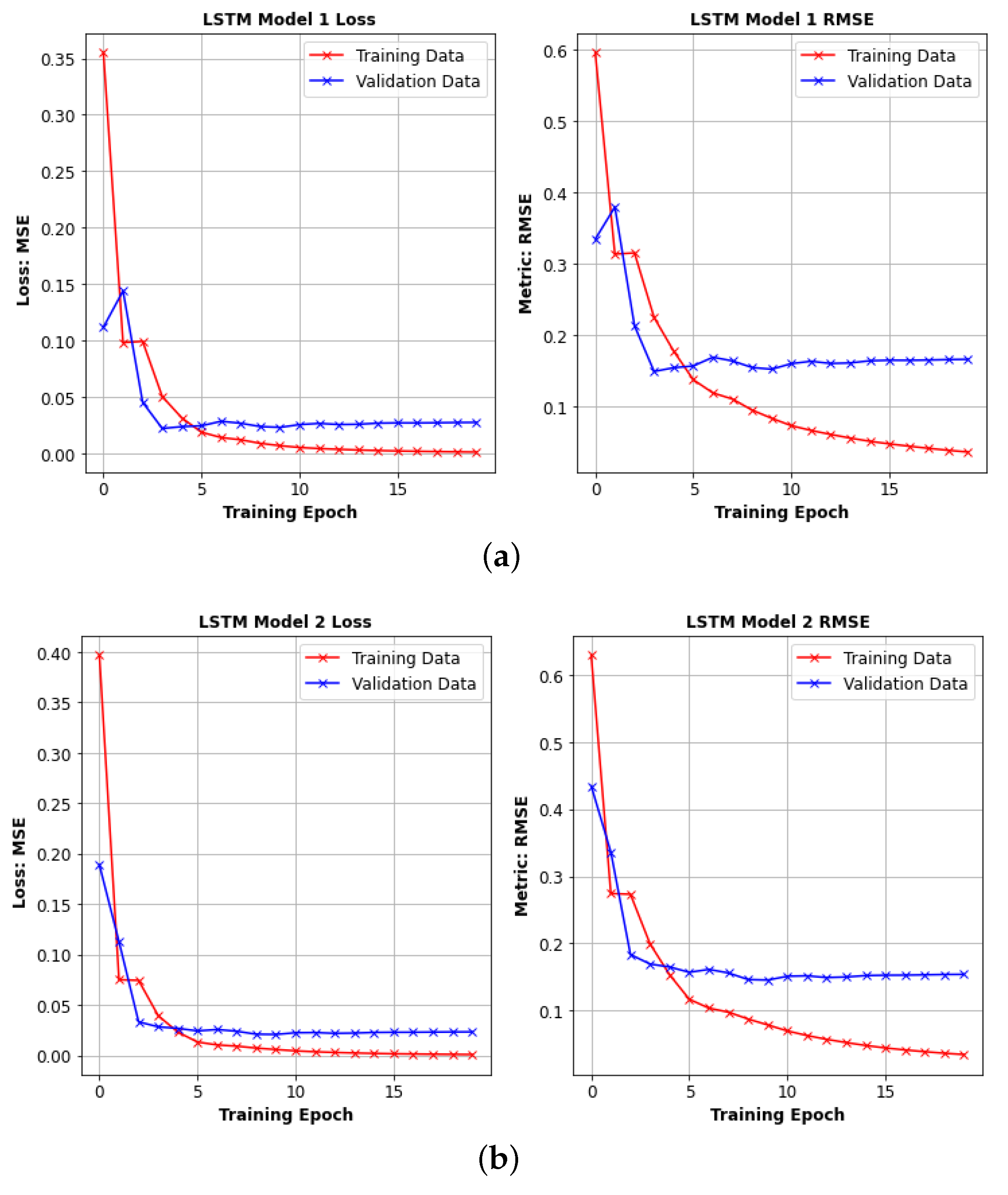
4.4. Long Short Term Memory Networks (LSTMs)
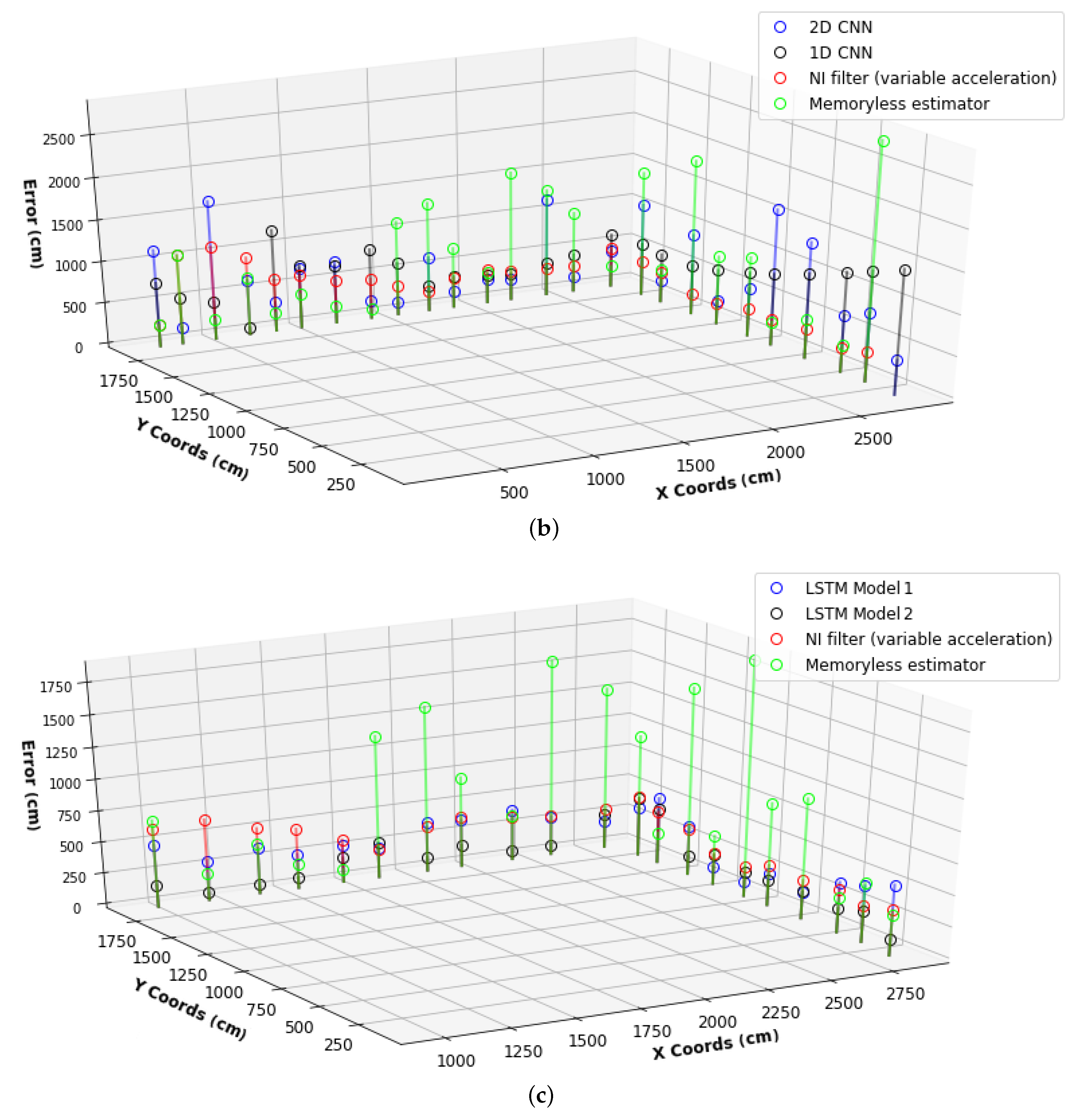
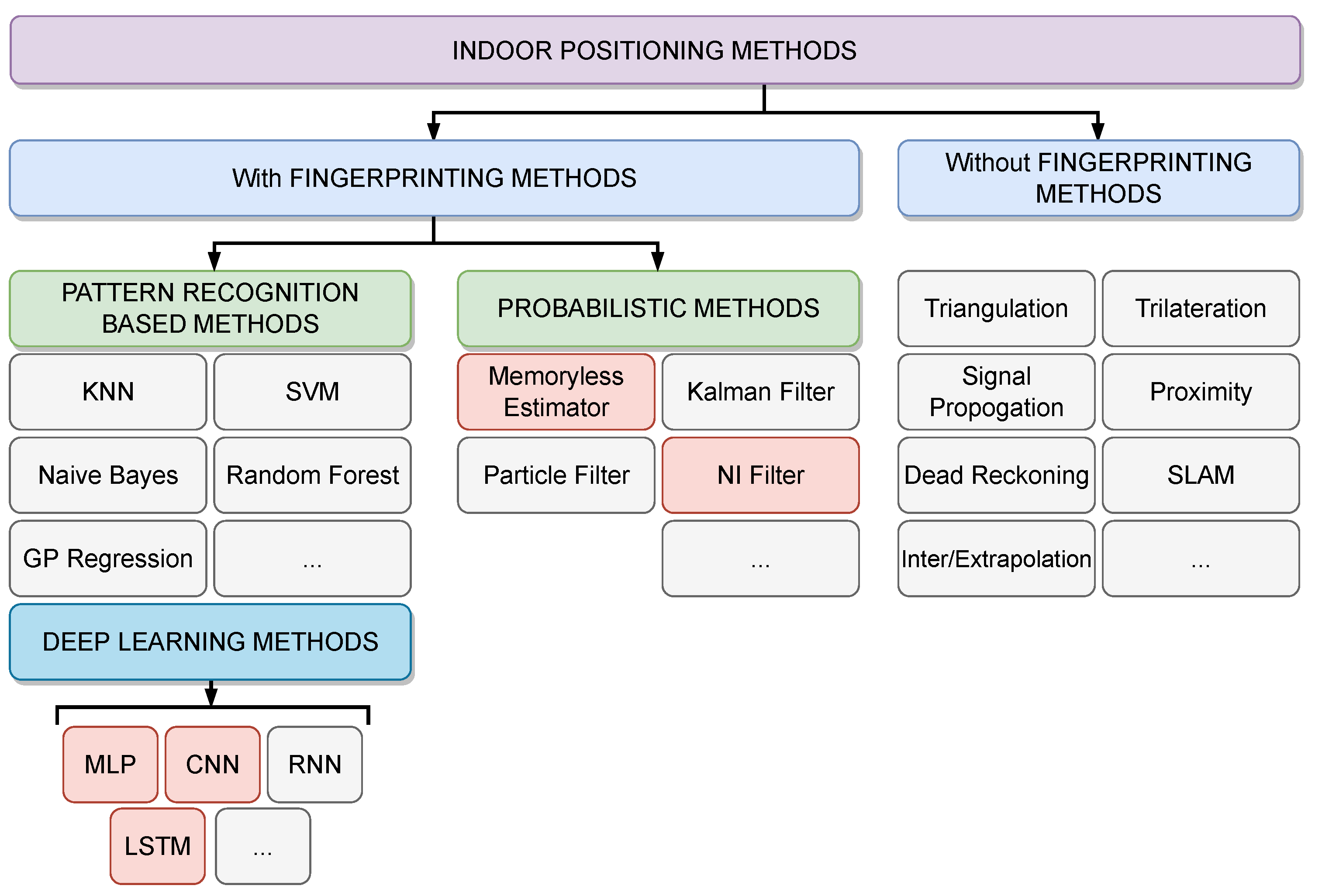
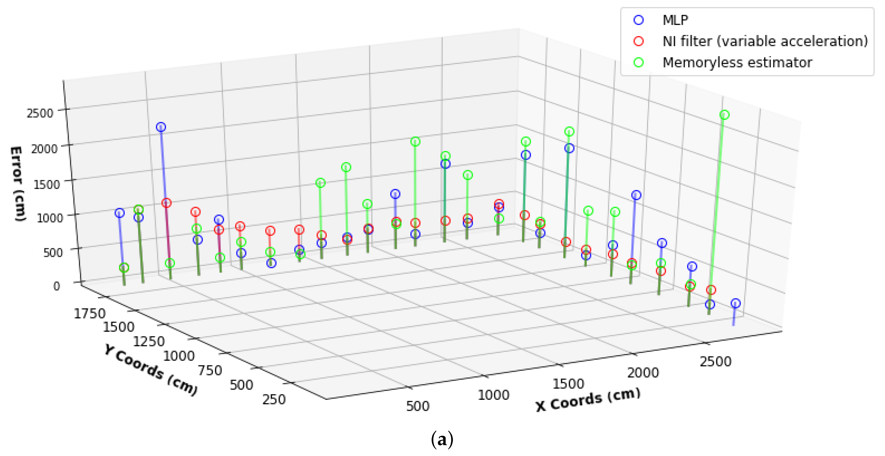
4.5. Alternative Probabilistic Techniques (Memoryless Estimator and NI Filter)
5. Experiments
5.1. Hyperparameters
5.2. Hyperparameter Tuning Process
6. Results
6.1. First stage HPO results
6.2. Second Stage HPO Results
7. Conclusions
Author Contributions
Funding
Institutional Review Board Statement
Informed Consent Statement
Data Availability Statement
Conflicts of Interest
References
- Voth, D. A new generation of military robots. IEEE Intell. Syst. 2004, 19, 2–3. [Google Scholar] [CrossRef]
- Takahashi, M.; Suzuki, T.; Cinquegrani, F.; Sorbello, R.; Pagello, E. A mobile robot for transport applications in hospital domain with safe human detection algorithm. In Proceedings of the 2009 IEEE International Conference on Robotics and Biomimetics (ROBIO), Guilin, China, 19–23 December 2009; pp. 1543–1548. [Google Scholar]
- Meghdari, A.; Shariati, A.; Alemi, M.; Nobaveh, A.A.; Khamooshi, M.; Mozaffari, B. Design performance characteristics of a social robot companion “Arash” for pediatric hospitals. Int. J. Humanoid Robot. 2018, 15, 1850019. [Google Scholar] [CrossRef]
- Emken, J.L.; Wynne, J.H.; Harkema, S.J.; Reinkensmeyer, D.J. A robotic device for manipulating human stepping. IEEE Trans. Robot. 2006, 22, 185–189. [Google Scholar] [CrossRef] [Green Version]
- Pignolo, L. Robotics in neuro-rehabilitation. J. Rehabil. Med. 2009, 41, 955–960. [Google Scholar] [CrossRef] [Green Version]
- Hvilshøj, M.; Bøgh, S.; Madsen, O.; Kristiansen, M. The mobile robot “Little Helper”: Concepts, ideas and working principles. In Proceedings of the 2009 IEEE Conference on Emerging Technologies & Factory Automation, Palma de Mallorca, Spain, 22–25 September 2009; pp. 1–4. [Google Scholar]
- Yoo, K.; Ryu, H.; Choi, C. Control Architecture Design for an Gas Cutting Robot. In Proceedings of the 2008 Second International Conference on Future Generation Communication and Networking Symposia, Hainan, China, 13–15 December 2008; Volume 4, pp. 66–71. [Google Scholar]
- Forlizzi, J.; DiSalvo, C. Service robots in the domestic environment: A study of the roomba vacuum in the home. In Proceedings of the 1st ACM SIGCHI/SIGART Conference on Human-Robot Interaction, Salt Lake City, UT, USA, 2–3 March 2006; pp. 258–265. [Google Scholar]
- Palacin, J.; Salse, J.A.; Valgañón, I.; Clua, X. Building a mobile robot for a floor-cleaning operation in domestic environments. IEEE Trans. Instrum. Meas. 2004, 53, 1418–1424. [Google Scholar] [CrossRef]
- Han, B.O.; Kim, Y.H.; Cho, K.; Yang, H.S. Museum tour guide robot with augmented reality. In Proceedings of the 2010 16th International Conference on Virtual Systems and Multimedia, Seoul, Korea, 20–23 October 2010; pp. 223–229. [Google Scholar]
- Martínez, D.; Moreno, J.; Tresanchez, M.; Teixidó, M.; Font, D.; Pardo, A.; Marco, S.; Palacín, J. Experimental application of an autonomous mobile robot for gas leak detection in indoor environments. In Proceedings of the 17th International Conference on Information Fusion (FUSION), Salamanca, Spain, 7–10 July 2014; pp. 1–6. [Google Scholar]
- Salman, R.; Willms, I.; Sakamoto, T.; Sato, T.; Yarovoy, A. Environmental imaging with a mobile UWB security robot for indoor localisation and positioning applications. In Proceedings of the 2013 European Radar Conference, Nuremberg, Germany, 9–11 October 2013; pp. 331–334. [Google Scholar]
- Kunhoth, J.; Karkar, A.; Al-Maadeed, S.; Al-Ali, A. Indoor positioning and wayfinding systems: A survey. Hum.-Centric Comput. Inf. Sci. 2020, 10, 1–41. [Google Scholar] [CrossRef]
- Mautz, R. Indoor positioning technologies. 2012. Available online: https://www.research-collection.ethz.ch/bitstream/handle/20.500.11850/54888/eth-5659-01.pdf (accessed on 4 July 2022).
- Alarifi, A.; Al-Salman, A.; Alsaleh, M.; Alnafessah, A.; Al-Hadhrami, S.; Al-Ammar, M.A.; Al-Khalifa, H.S. Ultra wideband indoor positioning technologies: Analysis and recent advances. Sensors 2016, 16, 707. [Google Scholar] [CrossRef]
- Al Nuaimi, K.; Kamel, H. A survey of indoor positioning systems and algorithms. In Proceedings of the 2011 International Conference on Innovations in Information Technology, Abu Dhabi, United Arab Emirates, 25–27 April 2011; pp. 185–190. [Google Scholar]
- Gu, Y.; Lo, A.; Niemegeers, I. A survey of indoor positioning systems for wireless personal networks. IEEE Commun. Surv. Tutorials 2009, 11, 13–32. [Google Scholar] [CrossRef] [Green Version]
- Yamagishi, S.; Jing, L. Pedestrian Dead Reckoning with Low-Cost Foot-Mounted IMU Sensor. Micromachines 2022, 13, 610. [Google Scholar] [CrossRef]
- Plataniotis, K.; Regazzoni, C. Visual-centric surveillance networks and services [Guest Editorial]. IEEE Signal Process. Mag. 2005, 22, 12–15. [Google Scholar] [CrossRef]
- Yang, B.; Li, J.; Shao, Z.; Zhang, H. Robust UWB Indoor Localization for NLOS Scenes via Learning Spatial-Temporal Features. IEEE Sensors J. 2022, 22, 7990–8000. [Google Scholar] [CrossRef]
- Machaj, J.; Brida, P.; Matuska, S. Proposal for a Localization System for an IoT Ecosystem. Electronics 2021, 10, 3016. [Google Scholar] [CrossRef]
- Poulose, A.; Han, D.S. UWB indoor localization using deep learning LSTM networks. Appl. Sci. 2020, 10, 6290. [Google Scholar] [CrossRef]
- Nagah Amr, M.; ELAttar, H.M.; Abd El Azeem, M.H.; El Badawy, H. An enhanced indoor positioning technique based on a novel received signal strength indicator distance prediction and correction model. Sensors 2021, 21, 719. [Google Scholar] [CrossRef] [PubMed]
- Ramirez, R.; Huang, C.Y.; Liao, C.A.; Lin, P.T.; Lin, H.W.; Liang, S.H. A Practice of BLE RSSI Measurement for Indoor Positioning. Sensors 2021, 21, 5181. [Google Scholar] [CrossRef]
- Harter, A.; Hopper, A. A distributed location system for the active office. IEEE Netw. 1994, 8, 62–70. [Google Scholar] [CrossRef]
- Tamas, L.; Lazea, G.; Popa, M.; Szoke, I.; Majdik, A. Laser based localization techniques for indoor mobile robots. In Proceedings of the 2009 Advanced Technologies for Enhanced Quality of Life, Iasi, Romania, 22–26 July 2009; pp. 169–170. [Google Scholar]
- Hazas, M.; Hopper, A. Broadband ultrasonic location systems for improved indoor positioning. IEEE Trans. Mob. Comput. 2006, 5, 536–547. [Google Scholar] [CrossRef] [Green Version]
- Uradzinski, M.; Guo, H.; Liu, X.; Yu, M. Advanced indoor positioning using zigbee wireless technology. Wirel. Pers. Commun. 2017, 97, 6509–6518. [Google Scholar] [CrossRef]
- Alatise, M.B.; Hancke, G.P. Pose estimation of a mobile robot based on fusion of IMU data and vision data using an extended Kalman filter. Sensors 2017, 17, 2164. [Google Scholar] [CrossRef] [Green Version]
- Poulose, A.; Han, D.S. Hybrid indoor localization using IMU sensors and smartphone camera. Sensors 2019, 19, 5084. [Google Scholar] [CrossRef] [Green Version]
- Leppäkoski, H.; Collin, J.; Takala, J. Pedestrian navigation based on inertial sensors, indoor map, and WLAN signals. J. Signal Process. Syst. 2013, 71, 287–296. [Google Scholar] [CrossRef]
- Zhuang, Y.; El-Sheimy, N. Tightly-coupled integration of WiFi and MEMS sensors on handheld devices for indoor pedestrian navigation. IEEE Sensors J. 2015, 16, 224–234. [Google Scholar] [CrossRef]
- Kim, D.H.; Kwon, G.R.; Pyun, J.Y.; Kim, J.W. NLOS identification in UWB channel for indoor positioning. In Proceedings of the 2018 15th IEEE Annual Consumer Communications Networking Conference (CCNC), Las Vegas, NV, USA, 12–15 January 2018; pp. 1–4. [Google Scholar] [CrossRef]
- Kushki, A.; Plataniotis, K.N.; Venetsanopoulos, A.N. Kernel-based positioning in wireless local area networks. IEEE Trans. Mob. Comput. 2007, 6, 689–705. [Google Scholar] [CrossRef] [Green Version]
- Karakuşak, M.Z.; Özdemir, K.; Aslantaş, V. The use of RSS and NI filtering for the Wireless indoor localization and tracking of mobile robots with different motion models. In Proceedings of the 2016 24th Signal Processing and Communication Application Conference (SIU), Zonguldak, Turkey, 16–19 May 2016; pp. 1709–1712. [Google Scholar]
- Jang, B.; Kim, H. Indoor positioning technologies without offline fingerprinting map: A survey. IEEE Commun. Surv. Tutorials 2018, 21, 508–525. [Google Scholar] [CrossRef]
- Kushki, A. A Cognitive Radio Tracking System for Indoor Environments. Ph.D. Thesis, University of Toronto, Toronto, ON, Canada, 2008. [Google Scholar]
- Ali-Loytty, S.; Perala, T.; Honkavirta, V.; Piché, R. Fingerprint Kalman filter in indoor positioning applications. In Proceedings of the 2009 IEEE Control Applications, (CCA) & Intelligent Control (ISIC), St. Petersburg, Russia, 8–10 July 2009; pp. 1678–1683. [Google Scholar]
- Yim, J.; Park, C.; Joo, J.; Jeong, S. Extended Kalman filter for wireless LAN based indoor positioning. Decis. Support Syst. 2008, 45, 960–971. [Google Scholar] [CrossRef]
- Yim, J.; Jeong, S.; Gwon, K.; Joo, J. Improvement of Kalman filters for WLAN based indoor tracking. Expert Syst. Appl. 2010, 37, 426–433. [Google Scholar] [CrossRef]
- Khalil, L.; Jung, P. Scaled unscented Kalman filter for RSSI-based indoor positioning and tracking. In Proceedings of the 2015 9th International Conference on Next Generation Mobile Applications, Services and Technologies, Cambridge, UK, 9–11 September 2015; pp. 132–137. [Google Scholar]
- Youssef, M.; Agrawala, A. The Horus location determination system. Wirel. Netw. 2008, 14, 357–374. [Google Scholar] [CrossRef]
- Roos, T.; Myllymäki, P.; Tirri, H.; Misikangas, P.; Sievänen, J. A probabilistic approach to WLAN user location estimation. Int. J. Wirel. Inf. Netw. 2002, 9, 155–164. [Google Scholar] [CrossRef]
- Kushki, A.; Plataniotis, K.; Venetsanopoulos, A.; Regazzoni, C. Radio map fusion for indoor positioning in wireless local area networks. In Proceedings of the 2005 7th International Conference on Information Fusion, Philadelphia, PA, USA, 25–28 July 2005; Volume 2, p. 8. [Google Scholar] [CrossRef]
- Chiou, Y.S.; Wang, C.L.; Yeh, S.C. An adaptive location estimator based on Kalman filtering for dynamic indoor environments. In Proceedings of the IEEE Vehicular Technology Conference, Montreal, QC, Canada, 25–28 September 2006; pp. 1–5. [Google Scholar]
- Güvenc, I. Enhancements to RSS based indoor tracking systems using Kalman filters. Master’s Thesis, University of New Mexico, Albuquerque, NM, USA, 2003. [Google Scholar]
- Chu, C.; Yang, S. A Particle Filter Based Reference Fingerprinting Map Recalibration Method. IEEE Access 2019, 7, 111813–111827. [Google Scholar] [CrossRef]
- Ladd, A.M.; Bekris, K.E.; Rudys, A.; Kavraki, L.E.; Wallach, D.S. Robotics-based location sensing using wireless ethernet. Wirel. Netw. 2005, 11, 189–204. [Google Scholar] [CrossRef]
- Gentile, C.; Klein-Berndt, L. Robust location using system dynamics and motion constraints. In Proceedings of the 2004 IEEE International Conference on Communications (IEEE Cat. No. 04CH37577), Paris, France, 20–24 June 2004; Volume 3, pp. 1360–1364. [Google Scholar]
- Belay Adege, A.; Yayeh, Y.; Berie, G.; Lin, H.p.; Yen, L.; Li, Y.R. Indoor localization using K-nearest neighbor and artificial neural network back propagation algorithms. In Proceedings of the 2018 27th Wireless and Optical Communication Conference (WOCC), Hualien, Taiwan, 30 Apri–1 May 2018; pp. 1–2. [Google Scholar] [CrossRef]
- Yoo, J.; Park, J. Indoor localization based on Wi-Fi received signal strength indicators: Feature extraction, mobile fingerprinting, and trajectory learning. Appl. Sci. 2019, 9, 3930. [Google Scholar] [CrossRef] [Green Version]
- Chriki, A.; Touati, H.; Snoussi, H. SVM-based indoor localization in wireless sensor networks. In Proceedings of the 2017 13th International Wireless Communications and Mobile Computing Conference (IWCMC), Valencia, Spain, 26–30 June 2017; pp. 1144–1149. [Google Scholar]
- Shi, K.; Ma, Z.; Zhang, R.; Hu, W.; Chen, H. Support vector regression based indoor location in IEEE 802.11 environments. Mob. Inf. Syst. 2015, 2015, 295652. [Google Scholar] [CrossRef] [Green Version]
- Song, C.; Wang, J.; Yuan, G. Hidden naive bayes indoor fingerprinting localization based on best-discriminating ap selection. ISPRS Int. J. Geo-Inf. 2016, 5, 189. [Google Scholar] [CrossRef]
- Wu, Z.; Xu, Q.; Li, J.; Fu, C.; Xuan, Q.; Xiang, Y. Passive Indoor Localization Based on CSI and Naive Bayes Classification. IEEE Trans. Syst. Man, Cybern. Syst. 2018, 48, 1566–1577. [Google Scholar] [CrossRef]
- Lee, S.; Kim, J.; Moon, N. Random forest and WiFi fingerprint-based indoor location recognition system using smart watch. Hum.-Centric Comput. Inf. Sci. 2019, 9, 1–14. [Google Scholar] [CrossRef]
- Wang, Y.; Xiu, C.; Zhang, X.; Yang, D. WiFi indoor localization with CSI fingerprinting-based random forest. Sensors 2018, 18, 2869. [Google Scholar] [CrossRef] [Green Version]
- Zhao, F.; Huang, T.; Wang, D. A Probabilistic Approach for WiFi Fingerprint Localization in Severely Dynamic Indoor Environments. IEEE Access 2019, 7, 116348–116357. [Google Scholar] [CrossRef]
- Tao, Y.; Yan, R.; Zhao, L. An Effective Fingerprint-Based Indoor Positioning Algorithm Based on Extreme Values. ISPRS Int. J. Geo-Inf. 2022, 11, 81. [Google Scholar] [CrossRef]
- Prasad, K.N.R.S.V.; Hossain, E.; Bhargava, V.K. Machine Learning Methods for RSS-Based User Positioning in Distributed Massive MIMO. IEEE Trans. Wirel. Commun. 2018, 17, 8402–8417. [Google Scholar] [CrossRef]
- Hsieh, C.H.; Chen, J.Y.; Nien, B.H. Deep learning-based indoor localization using received signal strength and channel state information. IEEE Access 2019, 7, 33256–33267. [Google Scholar] [CrossRef]
- Poulose, A.; Han, D.S. Hybrid Deep Learning Model Based Indoor Positioning Using Wi-Fi RSSI Heat Maps for Autonomous Applications. Electronics 2021, 10, 2. [Google Scholar] [CrossRef]
- Liu, Z.; Dai, B.; Wan, X.; Li, X. Hybrid wireless fingerprint indoor localization method based on a convolutional neural network. Sensors 2019, 19, 4597. [Google Scholar] [CrossRef] [PubMed] [Green Version]
- Sinha, R.S.; Hwang, S.H. Comparison of CNN applications for RSSI-based fingerprint indoor localization. Electronics 2019, 8, 989. [Google Scholar] [CrossRef] [Green Version]
- Mittal, A.; Tiku, S.; Pasricha, S. Adapting convolutional neural networks for indoor localization with smart mobile devices. In Proceedings of the 2018 on Great Lakes Symposium on VLSI, Chicago, IL, USA, 23–25 May 2018; pp. 117–122. [Google Scholar]
- Soro, B.; Lee, C. Joint time-frequency RSSI features for convolutional neural network-based indoor fingerprinting localization. IEEE Access 2019, 7, 104892–104899. [Google Scholar] [CrossRef]
- Yang, X.; Chen, D.; Huai, J.; Cao, X.; Zhuang, Y. An improved wireless positioning algorithm based on the LSTM network. In Proceedings of the China Satellite Navigation Conference (CSNC 2021), Nanchang, China, 26–28 May 2021; pp. 616–627. [Google Scholar]
- Lee, G. Recurrent Neural Network-Based Hybrid Localization for Worker Tracking in an Offshore Environment. Appl. Sci. 2020, 10, 4721. [Google Scholar] [CrossRef]
- Hoang, M.T.; Yuen, B.; Dong, X.; Lu, T.; Westendorp, R.; Reddy, K. Recurrent neural networks for accurate RSSI indoor localization. IEEE Internet Things J. 2019, 6, 10639–10651. [Google Scholar] [CrossRef] [Green Version]
- NetSurveyor. Available online: http://nutsaboutnets.com/netsurveyor-wifi-scanner/ (accessed on 4 July 2022).
- Bahl, P.; Padmanabhan, V.N. RADAR: An in-building RF-based user location and tracking system. In Proceedings of the Nineteenth Annual Joint Conference of the IEEE Computer and Communications Societies (Cat. No. 00CH37064), Tel Aviv, Israel, 26–30 March 2000; Volume 2, pp. 775–784. [Google Scholar]
- Alsindi, N.A.; Alavi, B.; Pahlavan, K. Measurement and modeling of ultrawideband TOA-based ranging in indoor multipath environments. IEEE Trans. Veh. Technol. 2008, 58, 1046–1058. [Google Scholar] [CrossRef]
- Url-1. Available online: https://www.mathworks.com/content/dam/mathworks/mathworks-dot-com/images/events/matlabexpo/nl/2019/nl-ai-techniques-matlab-signal-time-series-text-data-mw.pdf (accessed on 4 July 2022).
- Feurer, M.; Hutter, F. Hyperparameter optimization. In Automated Machine Learning; Springer: Cham, Switzerland, 2019; pp. 3–33. [Google Scholar]
- Bergstra, J.; Bengio, Y. Random search for hyper-parameter optimization. J. Mach. Learn. Res. 2012, 13, 281–305. [Google Scholar]
- Frazier, P.I. A tutorial on Bayesian optimization. arXiv 2018, arXiv:1807.02811. [Google Scholar]
- Li, L.; Jamieson, K.; DeSalvo, G.; Rostamizadeh, A.; Talwalkar, A. Hyperband: A novel bandit-based approach to hyperparameter optimization. J. Mach. Learn. Res. 2017, 18, 6765–6816. [Google Scholar]


| Parameters | Ranges [min : max : step size] |
|---|---|
| #layer size #hidden layer | [2 : 10 : 1] |
| #lag time-steps | [1 : 4 : 1] |
| #memory units | [25 : 250 : 25] |
| #filters | [8 : 64 : 8] |
| #neurons per hidden layer | [32 : 1025 : 32] |
| kernel size | [2 : 5 : 1] |
| dropout | [0.1 : 0.9 : 0.1] |
| activation function | [“elu”, “sigmoid”, “relu”, “tanh”, “selu”] |
| dense (FC) layer | [32 : 1025 : 32] |
| batch size | [8 : 32 : 8] |
| learning rate | [0.1, 0.01, 0.001] |
| optimizers | [“Adam”, “RMSprop”, “Adagrad”, “SGD”] |
| #epochs | [10 : 50 : 10] |
| CWT scale length | [15 : 35 : 5] |
| MLP | 1D CNN | 2D CNN | |||||||
|---|---|---|---|---|---|---|---|---|---|
| Bayesian | Hyperband | Random | Bayesian | Hyperband | Random | Bayesian | Hyperband | Random | |
| scale length | 30 | 20 | 20 | 1 | 1 | 1 | 20 | 25 | 25 |
| layer_size | 10 | 7 | 3 | 10 | 9 | 9 | 2 | 3 | 9 |
| dense layer (#neurons/filters, activation, dropout) | (1024, E, 0.9) | (416, S, 0.5) | (160, Sg, 0.6) | (16, S, 0.9) | (56, R, 0.2) | (56, R, 0.5) | (32, R, 0.1) | (48, R, 0.6) | (56, Sg, 0.7) |
| (640, E, 0.1) | (448, R, 0.3) | (768, Sg, 0.3) | (64, R, 0.4) | (16, T, 0.4) | (24, S, 0.4) | (64, E, 0.1) | (40, T, 0.2) | (48, S, 0.7) | |
| (32, Sg, 0.1) | (896, E, 0.6) | (352, R, 0.5) | (64, E, 0.9) | (48, E, 0.4) | (48, S, 0.6) | (56, R, 0.9) | (40, E, 0.2) | ||
| (32, R, 0.4) | (128, T, 0.5) | (2, L) | (64, E, 0.9) | (48, S, 0.8) | (32, T, 0.3) | (24, T, 0.4) | |||
| (1024, R, 0.1) | (928, T, 0.3) | (64, E, 0.9) | (16, S, 0.1) | (56, E, 0.7) | (16, R, 0.4) | ||||
| (32, R, 0.1) | (928, T, 0.2) | (24, R, 0.9) | (24, R, 0.8) | (24, R, 0.6) | (16, E, 0.7) | ||||
| (32, R, 0.1) | (448, S, 0.3) | (8, R, 0.1) | (32, Sg, 0.8) | (24, E, 0.3) | (32, E, 0.6) | ||||
| (32, R, 0.1) | (2, L) | (8,R, 0.1) | (16, T, 0.7) | (56, Sg, 0.7) | (8, R, 0.1) | ||||
| (32, R, 0.1) | (8, R, 0.1) | (40, S, 0.1) | (8, R, 0.1) | (64, S, 0.2) | |||||
| (576, R, 0.2) | (8, R, 0.1) | ||||||||
| (2, L) | |||||||||
| dense (FC) layer | (1024, E, 0.1) | (416, R, 0.2) | (608, S, 0.3) | (32, E, 0.1) | (928, E, 0.2) | (640, E, 0.2) | |||
| kernel size | 4 | 3 | 3 | 4 | 3 | 3 | |||
| optimizer | Adam | Adam | Adam | Adam | RMSprop | Adam | Adam | Adam | Adam |
| learning_rate | 0.001 | 0.1 | 0.1 | 0.1 | 0.1 | 0.1 | 0.001 | 0.001 | 0.1 |
| batch_size | 8 | 24 | 32 | 24 | 24 | 8 | 8 | 8 | 16 |
| epochs | 50 | 10 | 30 | 50 | 20 | 30 | 10 | 30 | 50 |
| val_rmse (cm) | 6.32 | 7.37 | 7.36 | 5.47 | 6.36 | 5.51 | 6.48 | 6.70 | 5.51 |
| test_rmse (m) | 6.79 | 7.61 | 7.59 | 8.04 | 6.38 | 6.19 | 6.86 | 7.03 | 5.89 |
| test time | 0.12 | 0.07 | 0.07 | 0.17 | 0.14 | 0.10 | 0.18 | 0.18 | 0.16 |
| LSTM Model 1 (M1) and Model 2 (M2) | ||||||
|---|---|---|---|---|---|---|
| Bayesian Opt. | Hyperband | Random Search | ||||
| M1 | M2 | M1 | M2 | M1 | M2 | |
| lag_size | 3 | 1 | 3 | 3 | 3 | 3 |
| memory_unit | 175 | 250 | 175 | 200 | 200 | 75 |
| learning_rate | 0.1 | 0.1 | 0.1 | 0.01 | 0.01 | 0.01 |
| batch_size | 8 | 8 | 16 | 24 | 16 | 32 |
| optimizer | Adam | Adam | RMS | RMS | Adam | RMS |
| epochs | 50 | 50 | 20 | 30 | 20 | 40 |
| val_rmse (cm) | 0.13 | 0.10 | 0.14 | 0.12 | 0.13 | 0.11 |
| test_rmse (m) | 4.87 | 4.08 | 5.04 | 4.66 | 4.73 | 4.23 |
| Parameters’ Sets Based on First Stage Tuning Results | Grid Search Optimal Hyperparameters | |||
|---|---|---|---|---|
| MLP | 1D CNN | 2D CNN | ||
| #hidden layer #convolutional layer | [3, 7] [9] | 3 | 9 | 9 |
| #filter | [56, 64] | - | 56 | 64 |
| #neurons per hidden layer | [640, 1024] | (1 × 1024, 2 × 640) | - | - |
| kernel size | [3] | - | 3 | 3 × 3 |
| dropout (MLP) dropout (CNNs) | [0.1] [0.4] | 0.1 | 0.4 | 0.4 |
| activation function (MLP) activation function (CNNs) | [“elu”, “relu”, “sigmoid”] [“elu”, “relu”, “selu”] | “relu” | “selu” | “elu” |
| #neurons of dense layer | [608, 640, 720] | - | 608 | 720 |
| batch size | [8, 16] | 16 | 8 | 8 |
| learning rate | [0.1, 0.01, 0.001] | 0.1 | 0.001 | 0.001 |
| optimizer | Adam | Adam | Adam | Adam |
| epochs (MLP) epochs (CNNs) | [30, 40, 50] [30, 50] | 40 | 30 | 50 |
| CWT scale parameter (MLP) CWT scale parameter (2D CNN) | [20, 25, 30] [25, 30] | 20 | 1 | 30 |
| val_rmse (cm) | 4.80 ± 0.3 | 5.72 ± 0.14 | 4.51 ± 0.89 | |
| test_rmse (m) | 5.30 ± 0.02 | 5.39 ± 0.19 | 5.30 ± 0.44 | |
| LSTM | Model 1 | Model 2 | |
|---|---|---|---|
| Parameters’ Sets Based on First Stage Tuning Results | Fine Tuning (Grid Search) Optimal Hyperparameters | ||
| lag_size | [2, 3, 4] | 4 | 4 |
| memory_unit | [175, 200] | 175 | 175 |
| learning_rate | [0.1, 0.01] | 0.01 | 0.01 |
| batch_size | [8, 16, 32] | 8 | 8 |
| optimizer | [“Adam”, “RMSprop”] | Adam | Adam |
| epochs | [20, 30, 50] | 20 | 20 |
| val_rmse (cm) | 0.09 ± 0.07 | 0.07 ± 0.06 | |
| test_rmse (m) | 2.78 ± 0.04 | 1.73 ± 0.06 | |
| MLP | 1D CNN | 2D CNN | LSTM Model 1 | LSTM Model 2 | Memoryless Estimator | NI Constant Velocity | NI Constant Acceleration | NI Variable Acceleration | |
|---|---|---|---|---|---|---|---|---|---|
| Training time (s) (mean ± std) | 5.55 ± 0.28 | 27.91 ± 0.46 | 818.24 ± 4.00 | 1.36 ± 1.04 | 1.61 ± 1.48 | ||||
| Test time (s) | 0.08 | 0.12 | 0.38 | 0.05 | 0.05 | ||||
| Total number of parameters | 1,861,506 | 1,466,114 | 13,983,986 | 281,052 | 288,052 | ||||
| RMSE (m) (mean ± std) | 5.30 ± 0.02 | 5.39 ± 0.19 | 5.30 ± 0.44 | 2.78 ± 0.04 | 1.73 ± 0.06 | 10.35 | 6.5 | 5.33 | 5.2 |
Publisher’s Note: MDPI stays neutral with regard to jurisdictional claims in published maps and institutional affiliations. |
© 2022 by the authors. Licensee MDPI, Basel, Switzerland. This article is an open access article distributed under the terms and conditions of the Creative Commons Attribution (CC BY) license (https://creativecommons.org/licenses/by/4.0/).
Share and Cite
Karakusak, M.Z.; Kivrak, H.; Ates, H.F.; Ozdemir, M.K. RSS-Based Wireless LAN Indoor Localization and Tracking Using Deep Architectures. Big Data Cogn. Comput. 2022, 6, 84. https://doi.org/10.3390/bdcc6030084
Karakusak MZ, Kivrak H, Ates HF, Ozdemir MK. RSS-Based Wireless LAN Indoor Localization and Tracking Using Deep Architectures. Big Data and Cognitive Computing. 2022; 6(3):84. https://doi.org/10.3390/bdcc6030084
Chicago/Turabian StyleKarakusak, Muhammed Zahid, Hasan Kivrak, Hasan Fehmi Ates, and Mehmet Kemal Ozdemir. 2022. "RSS-Based Wireless LAN Indoor Localization and Tracking Using Deep Architectures" Big Data and Cognitive Computing 6, no. 3: 84. https://doi.org/10.3390/bdcc6030084
APA StyleKarakusak, M. Z., Kivrak, H., Ates, H. F., & Ozdemir, M. K. (2022). RSS-Based Wireless LAN Indoor Localization and Tracking Using Deep Architectures. Big Data and Cognitive Computing, 6(3), 84. https://doi.org/10.3390/bdcc6030084