Article

RSS-Based Wireless LAN Indoor Localization and Tracking Using Deep Architectures

by
Muhammed Zahid Karakusak
1,2,*,
Hasan Kivrak
3,
Hasan Fehmi Ates
4 and
Mehmet Kemal Ozdemir
4
1
Graduate School of Engineering and Natural Sciences, Istanbul Medipol University, 34810 Istanbul, Turkey
2
Department of Electronics Technology, Karabuk University, 78010 Karabuk, Turkey
3
Department of Computer Engineering, Karabuk University, 78050 Karabuk, Turkey
4
Department of Computer Engineering, Istanbul Medipol University, 34810 Istanbul, Turkey
*
Author to whom correspondence should be addressed.
Big Data Cogn. Comput. 2022, 6(3), 84; https://doi.org/10.3390/bdcc6030084
Submission received: 6 July 2022 / Revised: 28 July 2022 / Accepted: 1 August 2022 / Published: 8 August 2022
(This article belongs to the Topic Machine and Deep Learning)

Abstract

:
Wireless Local Area Network (WLAN) positioning is a challenging task indoors due to environmental constraints and the unpredictable behavior of signal propagation, even at a fixed location. The aim of this work is to develop deep learning-based approaches for indoor localization and tracking by utilizing Received Signal Strength (RSS). The study proposes Multi-Layer Perceptron (MLP), One and Two Dimensional Convolutional Neural Networks (1D CNN and 2D CNN), and Long Short Term Memory (LSTM) deep networks architectures for WLAN indoor positioning based on the data obtained by actual RSS measurements from an existing WLAN infrastructure in a mobile user scenario. The results, using different types of deep architectures including MLP, CNNs, and LSTMs with existing WLAN algorithms, are presented. The Root Mean Square Error (RMSE) is used as the assessment criterion. The proposed LSTM Model 2 achieved a dynamic positioning RMSE error of 1.73 m , which outperforms probabilistic WLAN algorithms such as Memoryless Positioning (RMSE: 10.35 m ) and Nonparametric Information (NI) filter with variable acceleration (RMSE: 5.2 m ) under the same experiment environment.

1. Introduction

Over the last few decades, there has been a rapid development of mobile robots in indoor and outdoor environments, where real-time pose estimation is one of the most important problems. Especially in indoor environments, mobile robots can be used for many different purposes. There exists studies for military purposes for bomb and mine scanning and demining [1], healthcare services [2,3], rehabilitation studies [4,5], factory and industrial areas [6,7], cleaning services [8,9], museum guidance [10], and other different fields [11,12]. In these frameworks, position estimation methods [13], which are discussed under the umbrella of indoor positioning and mobile robot localization technology, come into the picture. These methods are an essential part of location-based applications.
Indoor positioning technologies are another fundamental part of location-based applications. These technologies are classified based on sensor types [14], the infrastructure of the system that uses them [15], and other approaches found in the literature [16,17]. There is a need to take regard for the infrastructure; for example, Ref. [15] divided indoor positioning into building dependent and building independent technologies. Building independent technologies, such as dead reckoning [18] or image-based technologies [19], do not rely on any infrastructure in a building. On the other hand, building dependent indoor positioning systems are further classified into two types: those that require dedicated infrastructure radio frequency identification (RFID) [14], ultra wideband (UWB) [20,21,22], Bluetooth low energy (BLE) beacons [23,24], infrared [25], laser [26], ultrasonic [27], zigbee [28], and those that use existing infrastructure (Wi-Fi, cellular-based, Bluetooth). Several studies have proposed hybrid indoor localization technologies, which use hybrid data sources of inertial measurement unit (IMU), camera, pedestrian dead reckoning (PDR), and Wi-Fi, to address sensor errors from each sensor for better position estimation performance. Hybrid approaches, which combine IMU and vision data [29,30], as well as Wi-Fi RSS and PDR-based sensor data fusion [31,32], are also introduced.
Each sensor technology has its own major limitations, either for the accuracy, cost, computational complexity, or labor required. When existing network infrastructure is used, Wi-Fi has benefits over BLE beacons and UWB regarding the cost and labor for the installation of infrastructure. Like Wi-Fi, BLE does not require a mobile beacon (tag) when smartphone-embedded BLE antennas are available. However, for BLE the indoor site must be equipped with BLE transceivers. BLE has recently gained attention for its usage in hospitals, museums, and shopping malls, where the accuracy of several meters is sufficient. With new versions of Bluetooth, signal reliability, range, and speed are being improved for better indoor localization approaches. On the other hand, UWB is a relatively new approach, whose radio waves operate in extended frequency bands of 3–10 GHz. UWB works well with centimeter-level accuracy in short-range line-of-sight (LOS) radio environments. The UWB systems rely on additional hardware, such as certain transmitter devices and receiver tags. UWB might be suited for industrial applications requiring more accuracy than meter-level. However, the performance of UWB positioning also deteriorates when the signal reception is non-line-of-sight (NLOS). Similar to Wi-Fi-based approaches, alternative approaches need to be developed for UWB NLOS case scenarios [33]. An overview of UWB positioning technologies is discussed in detail in the review and research articles [15,21,22].
The aforementioned positioning techniques, except dead reckoning, require the installation of infrastructure, which might be costly in terms of hardware and other requirements in widespread deployments. That is why WLAN positioning is preferred over other indoor localization methods due to its cost-effectiveness and without need for any additional hardware. It is essentially based on the transmit-receive relationship of radio signals between access points (APs) and the agent.
Due to environmental constraints, unpredictable behavior of signal propagation, and random variations of RSS samples even at a fixed location, WLAN positioning indoors is a challenging task because the relation between Received Signal Strength (RSS) and position do not generally follow parametric forms. Moreover, there are NLOS conditions caused by the presence of static and dynamic obstacles. Furthermore, a closed-form expression or explicit RSS-position relationship is not available for indoor environments. Hence, the relationship between RSS and position is widely described based on previously collected measurement data using fingerprinting-based techniques or radio propagation modeling.
This study investigates the applicability of deep learning methods to wireless indoor localization problems. The deep learning-based approach is preferred with the aim of improving the existing algorithms’ position prediction performance and eliminating data pre-processing (e.g., feature selection/extraction steps; which need expertise in the field). This feature has enabled us to develop four different deep network models, namely Multi-Layer Perceptron (MLP), One and Two Dimensional Convolutional Neural Networks (1D CNN and 2D CNN), and Long Short Term Memory (LSTM). Root Mean Square Error (RMSE) has been used as the assessment criteria. We then compared the performance results with popular probabilistic-based approaches used in WLAN positioning on the data described in Section 3. In comparison to probabilistic methods, such as Memoryless Positioning [34] and Nonparametric Information (NI) filter with variable acceleration [35], LSTM Model 2 presented an improvement of 8.62 m (83.28%) and 3.47 m (66.73%) in dynamic positioning errors, respectively.
In particular, the contributions of the study are given as follows:
  • Four different deep network architectures of MLP, CNNs, and LSTMs are proposed and their performance results are compared with one another and with the existing probabilistic-based approaches.
  • Extensive experiments were carried out on real-world data to identify the optimum deep learning model parameters using proposed two-stage hyperparameter optimization (HPO) techniques (e.g., Bayesian Optimization, Hyperband, Random Search, and Grid Search).
  • A novel data set collected in the faculty building, consisting of two types of data in the form of stationary and walking data containing RSS measurements in XML format, was built. The collected RSS measurements were parsed and converted into a radio map, followed by the data preparation process. In order to eliminate the need for expertise in the field, the RSS image data set were obtained using Continuous Wavelet Transform (CWT) and also sequential data were generated to train the deep network models.
The next sections of the article are structured as follows: Section 2 provides the review of literature in WLAN static and dynamic positioning studies. The specifics regarding the data used are introduced in Section 3. Section 4 and Section 5 present the methods and experiments, respectively. Section 6 discusses the results of the experimental study. Finally, Section 7 concludes the study and lays out some approaches that can be investigated further.

2. Related Work

Various indoor positioning methods have been investigated by researchers. They can be broadly classified into two categories with or without fingerprinting methods as shown in Figure 1. The methods which do not require the construction of fingerprint matrices (radio map) rely on methods such as triangulation, trilateration, signal propagation, proximity, dead reckoning, Simultaneous localization and mapping (SLAM), and inter/extrapolation. For more information about the methods without fingerprinting, one can refer to [36]. On the other hand, most of the studies on fingerprinting methods are based on probabilistic methods and pattern recognition-based techniques [37]. Regarding probabilistic methods, research efforts are either performed with a parametric Kalman filter [38] and its variants [39,40,41] or nonparametric approaches [34,42].
Since RSS and position relationship does not follow a parametric form, nonparametric methods are extensively studied as a tool for WLAN positioning [43]. Nonparametric probabilistic estimation methods approximate the likelihood function from the fingerprint matrices; as they do not rely on parametric forms of the RSS densities at each reference point. A nonparametric Kernel Density Estimator (KDE) has been developed for modeling spatio-temporal RSS properties using the Minimum Mean Squared Error (MMSE) technique, which is also known as Memoryless MMSE positioning [44]. Furthermore, in order to increase positioning accuracy for dynamic positioning (tracking), RSS measurements are incorporated with knowledge of motion dynamics using the parametric Kalman filter [45,46], nonparametric Particle filter [47,48,49], and NI filter [37]. The study in [37] is then extended to work with different dynamic motion models in [35].
The other type of fingerprinting-based approach is based on pattern recognition methods that aim to use machine learning algorithms to approximate RSS-position characteristics. To this end, k-nearest neighbors (KNN) [50,51], Support Vector Machines (SVM) [52,53], Naive Bayes [54,55], Random Forest [56,57], Expectation-maximization (EM) algorithm [58], and Gaussian process (GP) regression [59,60] have been applied for both regression and classification. As we reviewed some of them, a nearest neighbor-based solution that uses RSS measurements was proposed for indoor positioning and achieved an average localization error of 2.2 m using mobile fingerprinting based on semi-supervised learning in a 47 m × 36 m area with 193 APs on 283 test data points [51]. Moreover, in [59], an extreme value-based method is proposed using GP regression to fit the RSS values of circles, which are obtained by using “Useful”-APs (the result of AP selection) and “Similar”-RPs (reference points). Different dynamic positioning errors are achieved at 1.81 m and 2.28 m , in two similar experiment areas with varying reference and test points detected over 100 APs.
In addition to the existing probabilistic and pattern recognition-based methods, research efforts have been increased recently to improve the quality of estimation accuracy using deep network architectures [61,62]. It is considered that these deep networks may have the ability to encode complex RSS-position relationships into model parameters. Therefore, the applicability of deep learning methods, which are known to have high performance in problems such as computer vision and natural language processing, is being investigated for wireless indoor static and dynamic positioning (tracking) problems. One of the well-known approaches to deep network architecture is CNN-based localization. In this work [61], 1D CNN classifies 16 reference points based on the RSS data from a number of APs which is undefined in the study. The average prediction accuracy is reported as 82.32%. Furthermore, the position estimation performance of the 1D CNN network, which works with 1D RSS data, can be improved by building 2D CNN networks relying on 2D data [63,64]. In those studies, 2D CNN captures higher dimensional dependencies on 2D data. Mittal et al. [65] present a framework based on the Pearson correlation coefficient for generating 2D features from RSS data for a CNN-based fingerprinting method. However, this approach assumes that there is a linear correlation between RSS values and positions, which is not suitable for the unpredictable variation of the RSS. The average localization error they achieved is around 2 m based on the RSS measurements taken from 30 different reference points. 5 samples are obtained at each point but the number of APs is not defined. Ref. [66] employs the CWT to obtain 2D time-frequency domain data from RSS samples to predict the closest reference points. The weighted average of the first three reference points that are greater than a defined threshold determines the estimated robot position. 36 APs’ RSS data per 21 reference points, each of which has 100 samples, were used in training. The learned model was then evaluated on 11 test points, and the average localization error was reported as less than 2 m . Another widely preferred approach would be to develop an LSTM-based model for estimating the position indoors. The study of [67] uses RSS differences between adjacent reference points with a step size of 3 m to reduce RSS variation over time within an area of 113 m × 43 m . The approach has a 3.57 m positioning error utilizing LSTM networks with a lag size of 4. Ref. [68] proposes an indoor positioning system in a static ship environment by fusing geomagnetic sensor values and RSS values from 21 APs using LSTM. The average error of the proposed method is 2.72 m , which achieved a 22% improvement compared to the KNN method. Additionally, study [69] exploits a time-series approach and proposes different types of Recurrent Neural Network (RNN) solutions using RSS-based fingerprinting to perform indoor localization. The achieved localization errors range from 0.75 m to 1.05 m with the collected data of 6 APs from 365 reference points for 175 test points.
In this paper, we propose a set of deep learning-based methods based on a practical, cost-effective, and real-world experimental data collection approach that does not require an infrastructure setup. The study aims to contribute to the field with the usage of four different deep network architectures of MLP, CNNs, and LSTMs, by making comparisons between them, and the two-stage HPO technique.
Moreover, we compared the performance of the deep learning-based indoor localization algorithms with the probabilistic-based approaches. We believe it would be unfair to directly claim to be better or worse than the existing studies as the environment the experiments were carried out in affects the performance greatly. Therefore, the comparison with other studies was not completed. Instead, we took the probabilistic-based approach in [35] as the basis for the comparisons. As the captured data is the same for both approaches, we believe that the comparison would be fair in terms of accuracy.

3. Data

The experimental data for indoor positioning is collected on the last floor of the Faculty of Engineering Building located in the center of the Karabuk University Campus, Karabuk, Turkey. The experimentation site’s dimensions are 20 m × 29 m. Furthermore, the study specifically focuses on RSS data, unlike channel state information (CSI), time of arrival (TOA), angle of arrival (AOA), etc., which require additional hardware or installation. For the RSS measurements, the existing WLAN infrastructure of the faculty is utilized. Thus, the locations of APs are non-customizable. No further APs installation was completed in addition to the existing installation, and the locations of the APs are also not known. Hence, this experimental setup provides a cost-effective practical approach and can be used in real-world applications that already have a WLAN infrastructure.

3.1. Data Collection

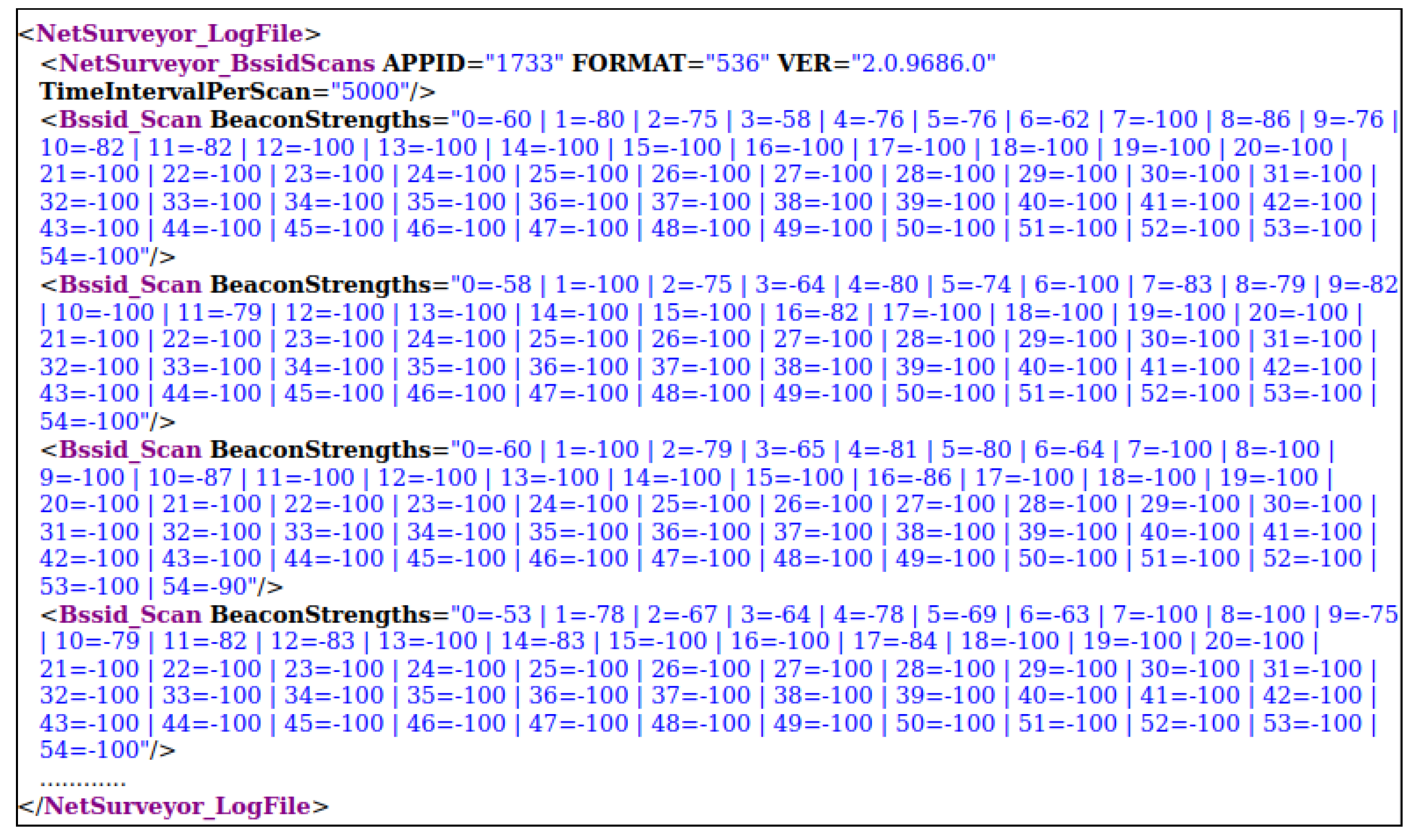
RSS measurements are captured via the open-source Netsurveyor program [70] distributed by Nuts About Nets LLC (Redmond, WA, USA), which provides an RSS sampling rate of about 2 samples/5 s. Data scans were updated approximately once every 5 s by using a Sony VAIO laptop, which has an Intel Centrino/Wireless-N 1000 Wi-Fi adaptor. The recorded data is in XML format (Figure 2) and consists of two scenarios: stationary and walking user data.
In the stationary user scenario, while collecting RSS measurements, the user remains stationary at all reference points. On the other hand, walking data is collected while the user is moving at walking speeds. This environment relies on setup settings similar to the existing literature in WLAN positioning in terms of the layout of the experimentation site and the location of reference points [71,72]. This is preferred in order to perform some performance comparisons with the existing state-of-the-art [35,37]. Based on the collected data, three separate data sets (training, validation, and testing) are created; as explained in the following subsections. Furthermore, the training and testing data sets were collected at different time frames to reflect the mismatch between training and testing conditions which are typical in real-life operations; since we cannot change the locations of APs.

3.1.1. Training and validation data

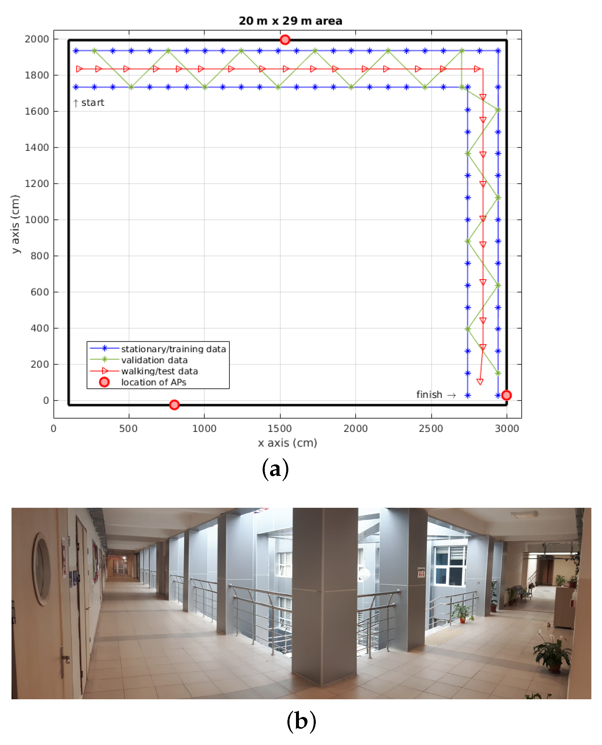
Training data was collected in a stationary scenario in the given environment. In order to avoid the extrapolation problem, a total of 78 reference points were placed every 100 cm on both sides of the corridor, and their coordinate information was recorded as shown in Figure 3a. The training data was collected at 78 reference points from detectable 45 APs throughout the floor at a rate of 1 sample/5 s. At each point, 10 samples are recorded for one orientation of the user to take environmental changes into account. With the collected data, a fingerprint matrix is developed as [35] F ( p i ) = r s s 1 1 , , r s s n 1 , , r s s 1 d , , r s s n d where i , d , and n are the number of reference points, the number of detectable APs, and the number of samples, respectively. This data was used to construct the radio map and thus, for building the proposed deep networks.
For the proposed network model, 23% of training data was reserved as validation data to be used for parameter tuning. As shown in Figure 3a, the green points represent a set of 18 reference points that can be considered as a saw tooth wave/zigzag shape, which is adopted to better assess the performance of the tracking of an agent/user.
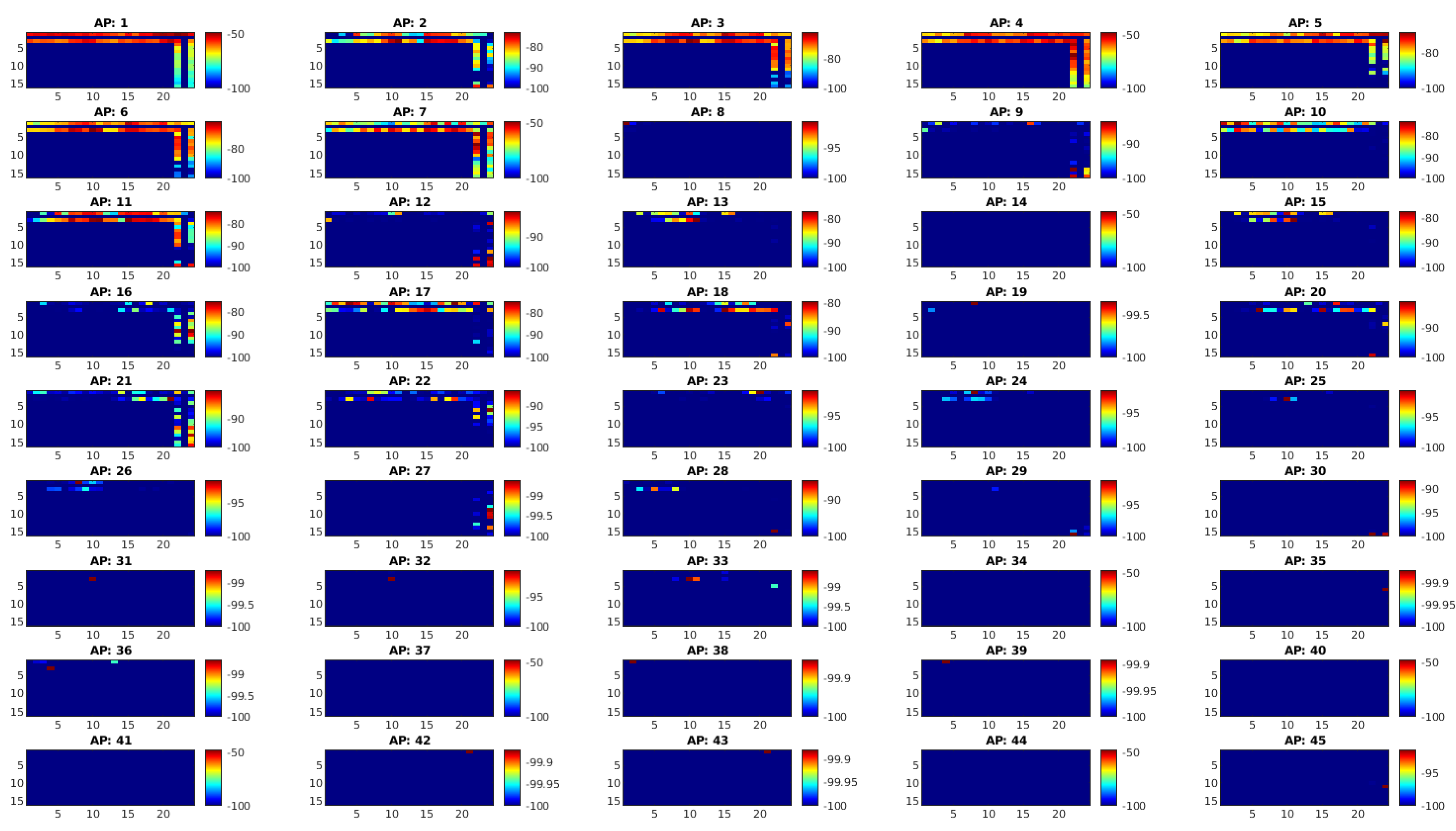
The detected 45 APs are depicted on the heat map in Figure 4. The heat map illustrates the Received Signal Strength Indicator (RSSI) distribution with a blue and red gradient, indicating higher and lower signal directions in the color bars from APs over a particular location surrounding the experimental site. It is the graphical representation of the obtained data. It is generated for the observation and understanding of the trends, outliers, and patterns in the data. RSS values are averaged over 10 samples for each reference point. This observation reinforces the need for an AP selection method to improve positioning errors because a subset of APs providing no available RSS, may result in biased estimates.

3.1.2. Testing Data

The test data was collected by the walking user, who followed a unique route between the reference points, excluding the reference points (Please see Figure 3a). This data collection method illustrates the mobility scenarios observed in tracking applications. Test measurements were recorded on a different day from the training and validation data to account for the impact of real-life environmental conditions on temporal changes, reflecting the mismatch between training and testing conditions. This data was used to assess the effectiveness of the suggested positioning strategies. The average route length was measured at 45 m (131 s) and the average velocity for the user was calculated to be 0.34 m/s. Test data was collected at 52 points for a single orientation at a rate of 1 sample/5 s.

3.2. Preparing Data

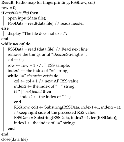
Since the data is in XML format as shown in Figure 2, it is required to convert the data (e.g., parsing XML files) to matrix format. So we can easily manage the RSS signals for developing models. A MATLAB data parser script is written as given in Algorithm 1.
Algorithm 1: Data parsing method for the recorded XML data using Netsurveyor program.
Bdcc 06 00084 i001
Then, we processed and cleaned the data so that it is in an appropriate format for the deep learning models by:
  • Removing and fixing outliers or inconsistencies caused by measurement errors of RSS data from APs. This was due to the natural variations in RSS data, it is likely to receive outlier data. A defined standard deviation from the mean was used to detect outliers assuming that the data had been coming from a Gaussian distribution. The outlier data was corrected with a time-average interpolation approach that was the mean of samples collected at each anchor point taken from each AP.
  • In the event of no data reception at a particular AP, missing RSS values were filled in with a value of −100 dB as the neutral integer to ensure data integrity.
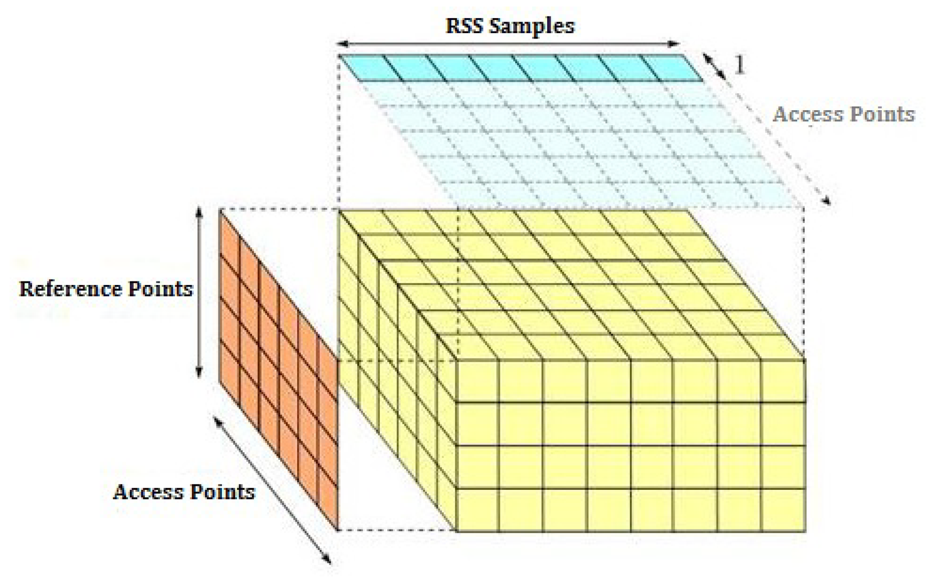
  • As a result, a 3D radio map with the dimension of 10 × 45 × 78 (samples per location, APs, reference points) was built and used in estimation algorithms as given in Figure 5.

4. Methods

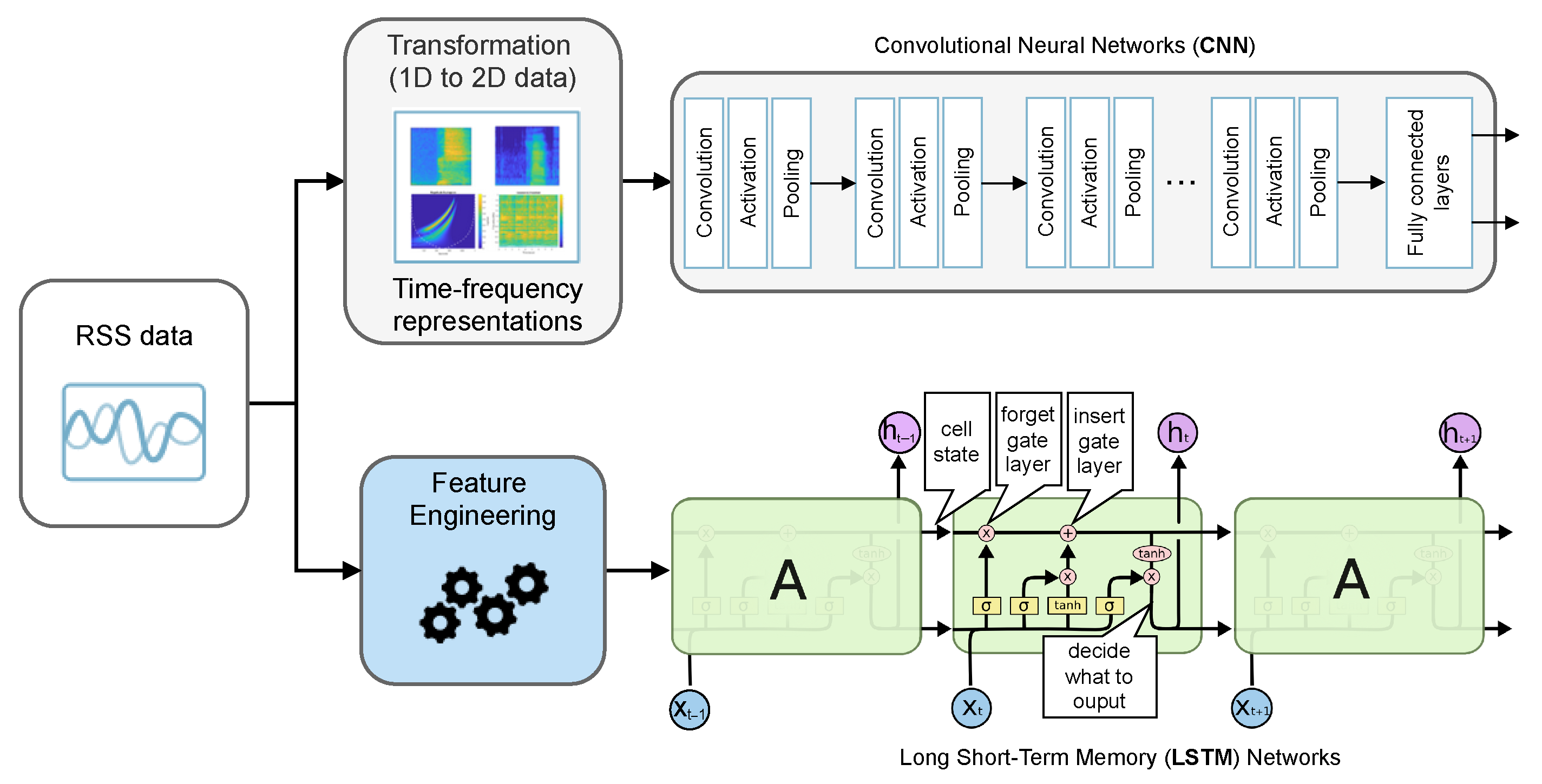
As the instantaneous RSS samples have random variations, the modeling of the RSS-position relationship becomes a challenging task. Deep learning methods are expected to learn a model of the RSS-position relationship for positioning a moving agent accurately by encoding complex environment factors into its model parameters. There are three widely used deep learning networks (MLP, CNN, LSTM) that researchers have focused on, particularly in recent years, to tackle a wide range of problems. As our data can be interpreted in the form of both tabular and time series data, all of the above methods are applicable to solving the Wi-Fi positioning problem. Figure 6 shows the proposed CNN and LSTM architectures to RSS-based WLAN positioning.
Moreover, Figure 7 shows the block diagram of the proposed deep network process, which visualizes the steps and relationships of principal parts of (a) data collection, (b) data preparation, (c) deep learning methods, and (d) model evaluation for WLAN positioning. As for the data collection, the proposed WLAN positioning model is implemented on top of existing WLAN infrastructures where no further APs are installed or any additional hardware is needed. The use of this setup enables the identification of real-world challenges and limitations of WLAN positioning as well as a fair assessment in realistic working environments. On the other hand, the study is a significant departure from existing literature [61,65,66,69]. The methodology of collecting test data for the current study is similar to the existing study of [69] since the data is gathered in a mobility scenario encountered in the tracking applications. However, it differs from other studies in [61,65,66] due to the stationary scenario experienced in the localization applications. In the data preparation strategy, the collected RSS measurements are parsed and converted into a radio map. The generated radio map was then used for the training of the learning models. Furthermore, in terms of deep learning methods, the current study has a similar approach with the usage of MLP and 1D CNN-based solution in [61], 2D CNN-based solution in [65,66], and LSTM-based solution in [69]. The current study differs from previous work in that it proposes different deepnet architectures of MLP, CNNs, and LSTMs by making comparisons between them as well as the two-stage HPO technique. Finally, for the model evaluation stage, the proposed deep learning models were trained using RMSE; a loss function commonly utilized in regressional tasks. Similarly, models were evaluated based on the RMSE assessment criteria.
The four main steps, or methods that we apply to solve the problem, are as follows:
  • Obtaining image data set of RSS fingerprint matrices.
  • Applying deep network models (i.e, MLP, 1D CNN, 2D CNN, LSTM) to predict the positions. Because we target the tracking problem, where the next location is highly dependent on the previous positions and the goal is to output a 2D spatial coordinate or position, WLAN positioning is formulated as a regression problem rather than a classification problem.
  • Carrying out extensive experiments to determine the impact of various deep learning system components by the hyperparameter tuning process.
  • Reporting the models’ performance. Positioning error is commonly evaluated as the euclidean distance between the actual position and its estimate. In this study, RMSE performance measure was used on training, validation, and test sets as shown in Equation (1). The RMSE measure was preferred since it penalized large errors and produces errors that were in the same unit as the prediction positions. The objective of the deep learning model was to minimize the RMSE loss function defined as the l 2 norm of difference in centimeters between all true positions ( p i ) and estimated positions ( p ^ i ).
    RMSE 1 N p n = 1 N p p i p ^ i 2
After an overview of all essential components of WLAN positioning is provided, the following subsections will describe how to create the RSS Image data set and present three deep learning methods for describing RSS-position relationships in detail.

4.1. RSS Time-Frequency Transformations (RSS Image Data Set)

There are several transformations that can be applied to signals to extract time-frequency representations as shown in Figure 8. We applied CWT, among other transforms, to extract time-frequency domain features of RSS signals. This is because the wavelet transform provides high resolution for non-periodic signals to exploit time-scale information [73]. CWT was applied to each sample considered as a time-series signal (Figure 9a), which corresponds to RSS measurements from available APs so that the length of the signal is 1 × d (the number of APs). Figure 9, which is given to observe the effects of CWT on RSS signals, represents the RSS signals data set and their CWT counterparts (RSS Image data set) computed with 35 scaling factors to be fed to train CNN models. The number of scaling factors determines the output image’s height. M scaling factor can be defined to obtain M × d time-scale representation from a 1D signal in order to form 2D images. When the scaling factor is applied to all signals obtained from reference points, it produces an N × ( M × d ) RSS Image data set that could be used in training. A collection of these images for all reference points generates the RSS Image data set as shown in Figure 9b. This 2D image data set is then used to train deep network models.

4.2. Multi-Layer Perceptron Neural Networks (MLPs)

MLPs are the most common type of neural network. An MLP is made up of one or more layers of neurons between the input and output. Layers of nodes between its input and output layers are called hidden layers. The input layer receives data, while multiple hidden layers with activation functions sequentially map inputs to a lower-dimensional space before the output layer, which makes a prediction. The output of the network has two neurons with linear activation functions which allow it to output predicted position values. The data should be presented in a tabular format. As such, our RSS image data set obtained by continuous wavelet time-scale representation of RSS was first normalized to 0–1 range. After that, the image in matrix form was reshaped into a 1D vector ( 1 , CWT scale parameter × RSS data ). MLPs are very flexible and general, but they are not linear classifiers and thus they can be used to learn any nonlinear mapping from inputs to outputs. This flexibility allows them to be applied to any type of data. After reducing the 2D time-scale representation of RSS information to a row of data, it is then fed to an MLP for feature extraction and prediction. In addition, MLP can also be used as a baseline method against the other deep learning models, against which analyses are performed, and thus the performance gains can be emphasized.

4.3. Convolutional Neural Networks (CNNs)

CNNs are a type of deep learning algorithm that consists of several stacked convolutional layers, each of which may perform a different purpose; being able to learn various aspects of input data. CNNs require a much lower amount of pre-processing than other classification techniques because the filters that characterize the input can be learned with enough training. 1D and 2D CNNs have similar properties and use the same methodology. The primary difference between these models is the dimension of the input data and the sliding method of the convolutional layers. 2D CNN models are developed for structured 2D data (i.e., data with 2D contextual dependencies). A similar approach can be applied to 1D data sequences, such as in the case of raw RSS data for WLAN positioning. A 1D CNN model can learn an internal representation of RSS observation sequences and can achieve comparable performance to models that require feature engineering; or expertise in the field. Since this study addresses a two-output regression task, the output layers of both models have two neurons for forcing the final output to predict x , y positions and the activation functions used in the output layers are linear.

4.4. Long Short Term Memory Networks (LSTMs)

The LSTM networks aim to learn the sequential dependence among the input variables; unlike other deep learning models such as MLP and CNNs for regression problems. Thus, LSTM is trained on a time-sequential data set with normalized inputs for the range of 0–1 to exploit the spatio-temporal correlation among them. Each data in the entire data set was framed together with RSS measurements of prior consecutive locations to predict the current position. The inputs (X) were reshaped into the 3D structure of [samples, timesteps, features] that LSTM models commonly expect. Moreover, in LSTMs, the memory length is defined by the number of lagged observations in terms of input time steps. The best value of memory length is determined by a HPO [74].
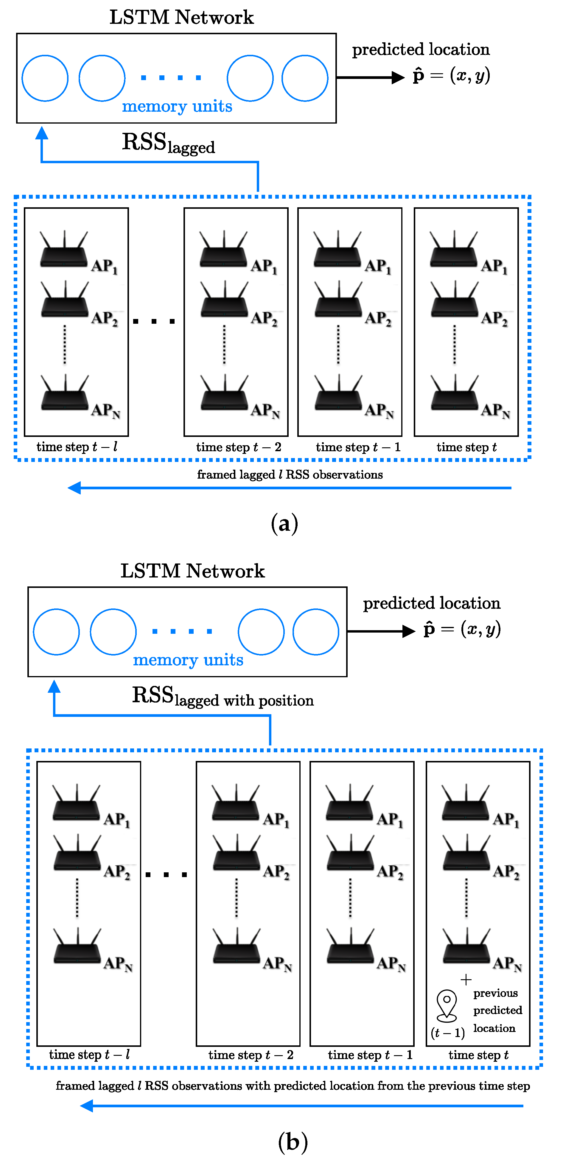
Two different LSTM models are proposed, as illustrated in Figure 10. Model 1 uses only a sequence of RSS observations, RSS lagged ,
RSS lagged = [ r s s t l ] , , [ r s s t 1 ] , [ r s s t ]
as input to generate an output location p ^ t at each time step t. Each RSS data point represents a different time step. The length of different time step RSS observations defines the lag size. Model 2, on the other hand, predicts the position p ^ t at each time step t using lagged RSS observations as well as the predicted position from the previous time step, RSS lwp .
RSS lwp = ( [ r s s t l ] ) , . . . , ( [ r s s t 1 ] ) , ( [ r s s t ] , p t 1 )
In this case, the first reference point needs to be excluded from the data set. This is because there is no prior predicted position to be packed with the lagged RSS data. Here, the goal was to determine whether the additional position information from the previous time step, t 1 , can help the LSTM model perform better or not.

4.5. Alternative Probabilistic Techniques (Memoryless Estimator and NI Filter)

In the literature, probabilistic techniques are also used as a tool for WLAN positioning [43]. The location estimation p ^ is usually computed using MMSE approach, p ^ = E { p | r } = P p f ( p | r ) d p , which is the expected value of the position p conditioned on the RSS measurements r . This equation requires the knowledge of the likelihood of density f ( r | p ) when it is rewritten using Bayes’ formula. The knowledge of the likelihood density was estimated using an RSS radio map. Since the parametric form of RSS and location is unknown, nonparametric KDE such as Gaussian Kernel is preferred [35]. This method is known as Memoryless MMSE positioning.
The knowledge of motion dynamics was also utilized as an additional source to improve the accuracy of the overall estimation. The joint approach both used RSS signal characteristics and dynamic modeling of the mobile user for the purpose of static and dynamic tracking of a mobile user’s location. This was performed by using the NI filter, which was introduced in [37]. Two algorithms for different dynamic motions were developed in [35] based on this overall approach. These algorithms were used for comparison purposes with the previously published methods. The implementation of these methods is based on a study conducted in [35].

5. Experiments

We built our deep network framework with one of the most popular frameworks, Keras. All experiments were conducted with the online cloud-based Jupyter Notebook Google Colaboratory (Colab). To evaluate the performance of the implemented networks, individual RMSE scores of reference points and total RMSE values were calculated. The networks were also compared in terms of complexity (e.g., average training and inference times, total number of model parameters). We used Memoryless and NI filter positioning approaches for the performance comparison with the proposed deep networks of MLP, CNNs, and LSTMs because they are popular methods used in WLAN positioning based on a fingerprinting approach. As with the comparison of other studies, we consider it to be unfair to directly claim to be better or worse than the existing studies; as the environments in which the experiments were taken affect the performance greatly. Instead, we took the fingerprinting-based approach tackled by [34,35] as the basis for the comparisons.

5.1. Hyperparameters

HPO had a great impact on the efficiency of deep learning models to develop the best accurate models. Identifying the optimal hyperparameter values given in Table 1 is usually an empirical process and is dependent on the input data set.
The large number of hidden or convolutional layers resulted in longer training/execution times and fewer hidden layers may have caused inaccurate results. Each layer, or filter, extracted a different set of features and contained unique information from the input. A large number of neurons, filters, or memory units per layer collected large amounts of information, whereas fewer neurons or filters can reduce the number of trainable parameters and computational costs in a single pass. Similarly, a large convolution kernel size can capture a large portion of information but increases the number of learnable parameters quadratically, which might make the models not cost-efficient enough.
Dropout regularization is a general approach for larger networks not to easily overfit the model on the training data. The CWT scale parameter formed the height of 2D RSS images. The number of lagged observations as input time steps defined the memory length in LSTMs. A larger memory length will include more historical data, but it will also result in more training times and the removal or non-positioning of the initial locations. Here, the optimal parameter set of the network was found by following a hyperparameter tuning process explained in Section 5.2.

5.2. Hyperparameter Tuning Process

Grid Search is the Brute-Force method to identify best performing hyperparameters as it evaluates all the required configurations. However, it suffers from high dimensionality. On the other hand, guided/directed search methods can be an alternative to model-free methods when the required number of function evaluations are costly as they work better and take less time than the Random Search [75]. One of the methods discussed under the umbrella of the guided search method is the Bayesian method, which is a probabilistic global optimization approach using a Gaussian process. It is especially useful for tasks when the evaluation function is computationally expensive and has fewer than 20 dimensions [76]. Thus, our problem dimension, as shown in Table 1, is appropriate. Furthermore, the Hyperband method is a variant of Random Search. However, it follows a bandit-based method among randomly sampled configurations with an exploration and exploitation strategy [77] and is known to perform good performance for deep neural networks [74].
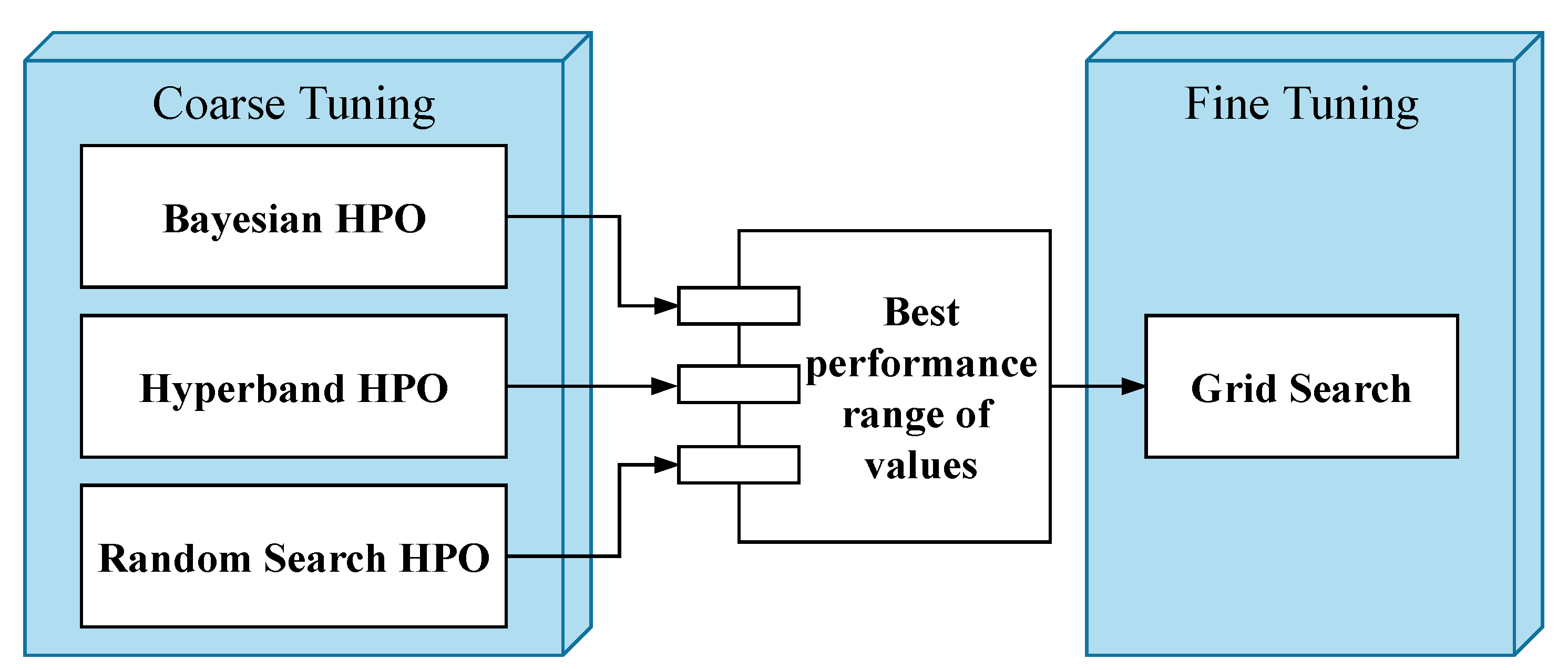
In light of the above considerations, we propose a two-stage coarse to fine strategy tuning process as shown in Figure 11. The first was carried out as coarse tuning within the specified ranges of values in Table 1 using Bayesian Optimization, Hyperband, and Random Search, which are the HPO methods used frequently in the literature [74]. The second one was conducted as fine-tuning by Grid Search around the promising parameters. In these experiments, the aim is to further improve/lift the performance of HPO methods with fine adjustments around the best-performing range of values produced by HPO methods.

6. Results

Due to the stochastic nature of the learning algorithms, our empirical experimentation was carried out by running the deepnet architectures for 3 times with each hyperparameter optimizer. Then, their average outcomes were compared with each other in order to identify the optimal hyperparameter values. In each case, the parameters resulting in the smallest RMSE (mean ± std) were selected.

6.1. First stage HPO results

The first stage of the hyperparameter tuning process was performed for MLP, 1D CNN, 2D CNN, and LSTM models in the specified range of parameter values given in Table 1. The first stage HPO results found by HPO methods for each deepnet are presented in Table 2.
In this experiment, we can get an idea of the optimum parameter range of hyperparameters and also agreements across several HPO methods. For the MLP model, there was a disagreement on the number of layers, neurons per layer, etc., but all three concluded that Adam is the best optimizer. For the 1D CNN case, there was not much difference between layer size and kernel size, and all three agreed that 0.1 was the optimal learning rate. Finally, for 2D CNN deepnet, all three had a consensus on the optimum optimizer and there was not a notable difference in the parameters of scale length and batch size. The results in Table 2 show that Bayesian Optimization returned the lowest RMSE score of 6.79 m for MLP, while the Random Search reported the minimum test RMSE for both 1D CNN and 2D CNN as 6.19 m and 5.89 m, respectively.
Similarly, the first stage HPO results on LSTM models (Model 1 and Model 2) for each optimization method are given in Table 3. While there are small differences in the other hyperparameters, all the three hyperparameter tuners have an agreement on the same lag length for Model 1. This might be interpreted as lag length having a great impact on prediction performance. It was also observed that there are pairwise agreements on the other parameters of Model 1 and between several hyperparameters of Model 2. Table 3 shows that Random Search achieved the lowest RMSE score of 4.73 m for Model 1, whereas a minimum RMSE of 4.08 m was achieved by Bayesian Optimization for Model 2. Thus, in the second stage, further analysis around the reported range of hyperparameters was performed using Grid Search to be confident in optimality.

6.2. Second Stage HPO Results

The performance comparison of MLP, 1D, and 2D CNN architectures for the set of best hyperparameter values found by Grid Search as a second stage tuning process is presented in Table 4.
The three hidden layer MLP network on 20 (CWT scale parameter) × 45 input images achieved a 5.30 m RMSE score. One of the hidden layers had 1024 and two of them had 640 neurons with a dropout rate of 0.1 , a learning rate of 0.1 , a batch size of 16, the activation function of RELU, and an Adam optimizer with 40 epochs. The input layer receives data while one or more hidden layers allow for different levels of abstraction, which affect the model and computational complexity as well as accuracy. MLP positioning accuracy was increased by 6.79 − 5.30 = 1.49 m (21.94%) with the Grid Search fine-tuning process compared to Bayesian Optimization, which achieved 6.79 m in the first stage.
Moreover, the architecture with nine 1D convolutional layers each having 56 filters with a kernel size of 3, a batch size of 8 on each 30 epochs, a dropout rate of 0.4, an activation function of SELU and Adam optimizer with 0.001 learning rate achieved 5.39 m RMSE. In each layer, a dropout layer was added for regularization and then flattened to feed a dense layer, which had 608 units. In comparison to the Random Search, which had the greatest score in the first stage, the Grid Search fine-tuning improved 1D CNN prediction performance by 6.19 − 5.39 = 0.8 m or 12.92%.
Furthermore, the 2D CNN architecture was constructed with a stack of nine convolution layers followed by a single fully-connected layer. Each convolutional layer has 64 filters with a kernel size of 3 × 3 that use the ELU activation functions to capture or extract features from 30 ( CWT scale parameter ) × 45 × 1 input images. 40% of the connections were ignored to avoid overfitting at the end of convolutional layers. The extracted features were then flattened before being fed into a fully-connected layer with 720 neurons. An Adam optimizer with a learning rate of 0.001 with 50 epochs on batch size 8 achieved 5.30 m tracking accuracy. The second stage Grid Search approach improved the first stage Random Search RMSE score by 5.89 − 5.30 = 0.59 m or 10.02%.
In addition to these, Table 5 shows the smaller search space explored by HPO methods used for first stage tuning as well as the top hyperparameter values of Model 1 and Model 2 chosen by Grid Search based on validation data. The best value of the lag length and memory unit, learning rate, batch size, and number of epochs, as well as the type of optimizer, is found for each model. As a result, Model 1 and Model 2 have the same architecture with a 4 lag length, a memory unit of 175, a learning rate of 0.01, a batch size of 8, and an Adam optimizer with 20 epochs achieving the best minimum RMSE score on the test data. With this two-stage strategy, the number of trials was reduced from 9600 to 216, which decreased the calculation and trials of Grid Search by a factor of 97.75% fewer trials.
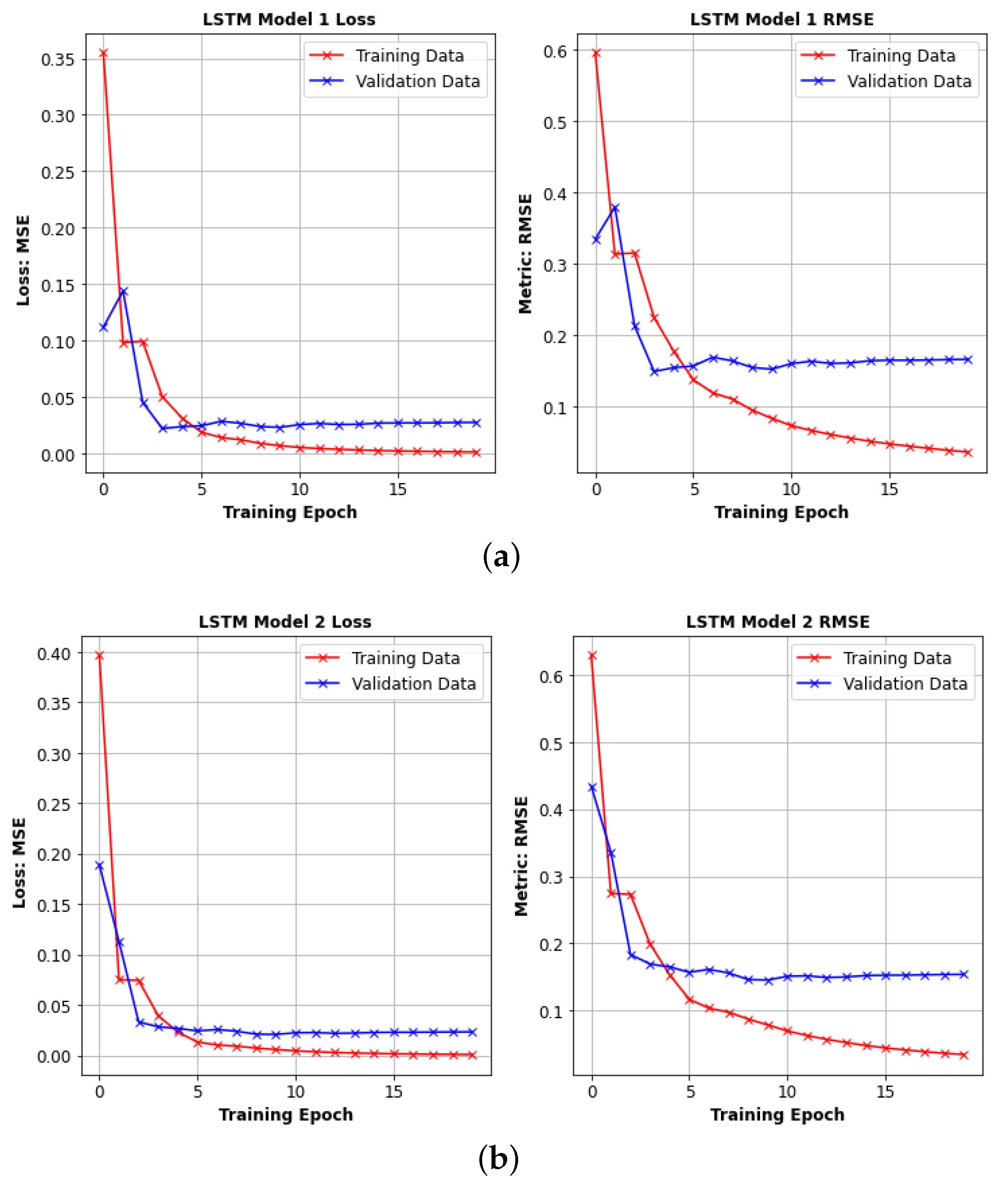
The learning performance of LSTM models over 20 epochs on both train and validation data sets are given in Figure 12. The training loss curves decrease until they stabilize and have a small gap with the validation loss, which shows a good fit. Furthermore, the fine-tuning process improved the Model 1 LSTM tracking performance by 4.73 2.78 = 1.95 m (41.23%) compared to Random Search which achieved the best score in the first stage. Model 2 outperformed Model 1 in terms of positioning accuracy, achieving 1.73 ± 0.06 m. Interestingly, the same sets of parameters were found for each model by the Grid Search, as shown in Table 5. In addition, the Grid Search improved Model 2’s performance by 4.08 1.73 = 2.35 m ( 57.60 % ) with fine-tuning of its parameters when compared to Bayesian Optimization, which got the highest score in the first stage. The overall results also indicated that there was a tendency for a decrease in the estimation error when the lag size was increased. In addition, Model 2 with a lag size of 1 at 50 epochs compared with Model 1 with a lag size of 4 at epoch size of 20 increased the prediction performance by approximately 3 % .
In summary, at the end of a two-stage HPO approach, the appropriate hyperparameters were found for each deep architecture developed for the problem of positioning and tracking in WLAN environments. Table 6 compares various deep networks, Memoryless, and the NI filter with its variants in terms of training and test times, the total number of parameters, and error statistics.
Here, all deep network models outperform Memoryless estimator and NI filter with the constant velocity dynamic model in terms of positioning accuracy. While MLP and 2D CNN approaches have similar performance, they both had better results when compared to the 1D CNN model. MLP also gives close results to the NI filter which uses a variable acceleration motion (dynamic) model. This indicates that the MLP model was able to capture the correlation between different scales of the CWT more successfully than CNNs. On the other hand, LSTM models outperform the MLP and NI filter. LSTM Model 2, compared to probabilistic methods (Memoryless, NI filter with variable acceleration), achieved an improvement of 8.62 m ( 83.28 % ) and 3.47 m ( 66.73 % ) in dynamic positioning errors, respectively. It is probable this improvement was due to the fact that capturing long-term temporal dependencies among RSS measurements results in considerable increases in positioning accuracy. Moreover, the estimation error was reduced to 1.73 m when RSS features were used with the previous time step predicted position (LSTM Model 2). The additional dynamic behavior of the user (e.g., position information) contributed to the estimation of a position. This shows that the RSS measurement and the position of the user are correlated over time. Furthermore, the network’s total number of parameters is defined by the input and output dimensions, number of layers, and number of units in each layer. Specifically, it is the sum of the connections between layers and biases in each layer. LSTM models and 1D CNN have fewer trainable parameters than other models because they are fed with raw RSS measurements, while MLP and 2D CNN are fed with 2D RSS images besides the effect of other parameters (e.g., layer size, number of neurons, and filters). Moreover, the 2D CNN model, which has nine layers each with 64 filters, is the most complex model with approximately 14 million parameters. On the other hand, LSTM had the lowest training and inference (test) times relative to the other models.
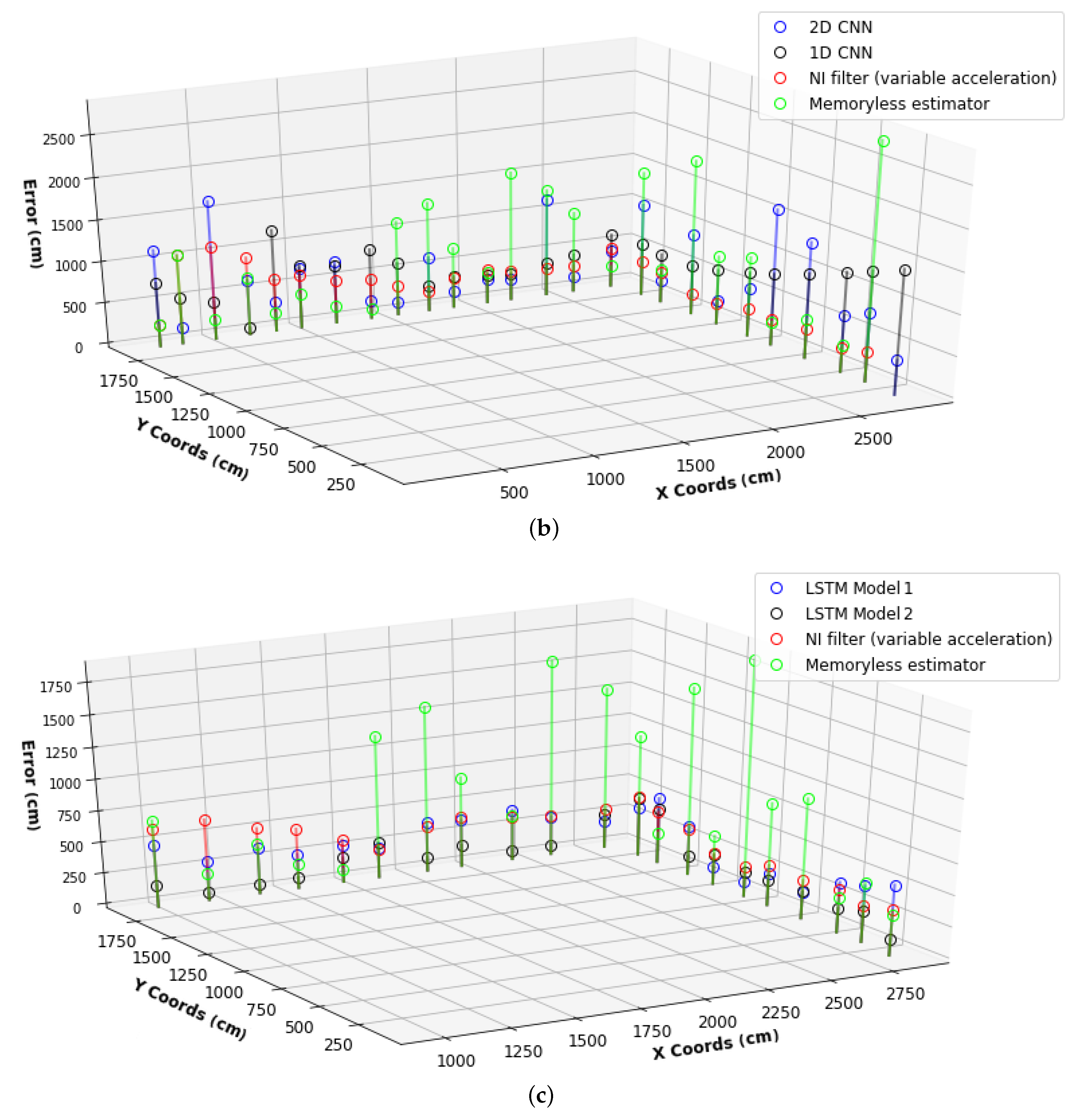
Finally, Figure 13 demonstrates the tracking error performance of MLP models, CNNs, LSTMs, the Memoryless estimator, and NI filter with a variable acceleration dynamic model on each test point. Z entries are shown as errors extending from the xy-plane, where X and Y are the tracking reference points in the xy-plane. Here, the estimation at the points close to the elevator and at the corners with a turn of 90 degrees surrounded by offices and classrooms resulted in the highest error rate. The error sources, such as multipath propagation and shadowing, caused an increase in the noise of the RSS and hence degradation of positioning accuracy. However, the inclusion of the dynamic motion model with the addition of position information was observed to improve the positioning accuracy, mitigating the difficulties caused by the mentioned error sources in the indoor environment.

7. Conclusions

This study focused on the problem of RSS-based WLAN indoor localization and tracking using deep architectures. Four deep neural networks were developed for position estimation in an indoor environment. When compared to the other deep networks, the LSTM network architecture achieved the best positioning performance while requiring significantly less training and inference time as well as complexity. Moreover, It can be concluded that the usage of lagged RSS observations, with the predicted location from the previous time step, refined LSTM network position accuracy. Furthermore, hyperparameters had a great effect on model performance. We recommend that when the dimension is high, HPO methods such as Bayesian optimization, Hyperband and Random search be a significantly greater choice due to their ability to evaluate faster. Grid Search can be an advantage to find the optimum hyperparameters if the search space is not so big. To utilize both approaches efficiently, we proposed and followed two-stage HPO, which is a combination of HPO methods with Grid Search optimization. We observed that Grid Search improved the first stage tuning of different models by a range of 10.02% to 57.60%.
In addition, we will include several strategies for generating RSS Image data sets by applying various transformations. Moreover, we hope to extend our LSTM network approach by using multiple output step predictions, which aim to predict more than one future position at a given point. This should lead to improvements in dynamic positioning accuracy since it can closely match with the dynamic model of pedestrian motion. Furthermore, if we can fuse different signal characteristics used for positioning such as RSS, TOA with multipath profile and knowledge of motion dynamics as an additional source, we expect to achieve more accurate results. In the case of the locations of APs being dynamic, it will be investigated whether the system needs to learn or adjust for this change for better accuracy. Additionally, the developed approach is also considered to be used for a new scenario by using a transfer learning approach to share the generalized knowledge.

Author Contributions

Conceptualization, M.Z.K.; methodology, M.Z.K. and H.K.; software, M.Z.K. and H.K.; data curation, M.Z.K.; writing—original draft preparation, M.Z.K.; writing—review and editing, H.K., H.F.A. and M.K.O.; funding acquisition, M.K.O. All authors have read and agreed to the published version of the manuscript.

Funding

The research leading to these results has received funding from the ECSEL Joint Undertaking in collaboration with the European Union’s H2020 Framework Programme (H2020/2014-2020) Grant Agreement-101007321-StorAIge and National Authority TUBITAK with project ID 121N350.

Institutional Review Board Statement

Not applicable.

Informed Consent Statement

Not applicable.

Data Availability Statement

The data presented in this study are available on request from the corresponding author. The data are not publicly available due to privacy.

Conflicts of Interest

The authors declare no conflict of interest. The funders had no role in the design of the study; in the collection, analyses, or interpretation of data; in the writing of the manuscript, or in the decision to publish the results.

References

  1. Voth, D. A new generation of military robots. IEEE Intell. Syst. 2004, 19, 2–3. [Google Scholar] [CrossRef]
  2. Takahashi, M.; Suzuki, T.; Cinquegrani, F.; Sorbello, R.; Pagello, E. A mobile robot for transport applications in hospital domain with safe human detection algorithm. In Proceedings of the 2009 IEEE International Conference on Robotics and Biomimetics (ROBIO), Guilin, China, 19–23 December 2009; pp. 1543–1548. [Google Scholar]
  3. Meghdari, A.; Shariati, A.; Alemi, M.; Nobaveh, A.A.; Khamooshi, M.; Mozaffari, B. Design performance characteristics of a social robot companion “Arash” for pediatric hospitals. Int. J. Humanoid Robot. 2018, 15, 1850019. [Google Scholar] [CrossRef]
  4. Emken, J.L.; Wynne, J.H.; Harkema, S.J.; Reinkensmeyer, D.J. A robotic device for manipulating human stepping. IEEE Trans. Robot. 2006, 22, 185–189. [Google Scholar] [CrossRef] [Green Version]
  5. Pignolo, L. Robotics in neuro-rehabilitation. J. Rehabil. Med. 2009, 41, 955–960. [Google Scholar] [CrossRef] [Green Version]
  6. Hvilshøj, M.; Bøgh, S.; Madsen, O.; Kristiansen, M. The mobile robot “Little Helper”: Concepts, ideas and working principles. In Proceedings of the 2009 IEEE Conference on Emerging Technologies & Factory Automation, Palma de Mallorca, Spain, 22–25 September 2009; pp. 1–4. [Google Scholar]
  7. Yoo, K.; Ryu, H.; Choi, C. Control Architecture Design for an Gas Cutting Robot. In Proceedings of the 2008 Second International Conference on Future Generation Communication and Networking Symposia, Hainan, China, 13–15 December 2008; Volume 4, pp. 66–71. [Google Scholar]
  8. Forlizzi, J.; DiSalvo, C. Service robots in the domestic environment: A study of the roomba vacuum in the home. In Proceedings of the 1st ACM SIGCHI/SIGART Conference on Human-Robot Interaction, Salt Lake City, UT, USA, 2–3 March 2006; pp. 258–265. [Google Scholar]
  9. Palacin, J.; Salse, J.A.; Valgañón, I.; Clua, X. Building a mobile robot for a floor-cleaning operation in domestic environments. IEEE Trans. Instrum. Meas. 2004, 53, 1418–1424. [Google Scholar] [CrossRef]
  10. Han, B.O.; Kim, Y.H.; Cho, K.; Yang, H.S. Museum tour guide robot with augmented reality. In Proceedings of the 2010 16th International Conference on Virtual Systems and Multimedia, Seoul, Korea, 20–23 October 2010; pp. 223–229. [Google Scholar]
  11. Martínez, D.; Moreno, J.; Tresanchez, M.; Teixidó, M.; Font, D.; Pardo, A.; Marco, S.; Palacín, J. Experimental application of an autonomous mobile robot for gas leak detection in indoor environments. In Proceedings of the 17th International Conference on Information Fusion (FUSION), Salamanca, Spain, 7–10 July 2014; pp. 1–6. [Google Scholar]
  12. Salman, R.; Willms, I.; Sakamoto, T.; Sato, T.; Yarovoy, A. Environmental imaging with a mobile UWB security robot for indoor localisation and positioning applications. In Proceedings of the 2013 European Radar Conference, Nuremberg, Germany, 9–11 October 2013; pp. 331–334. [Google Scholar]
  13. Kunhoth, J.; Karkar, A.; Al-Maadeed, S.; Al-Ali, A. Indoor positioning and wayfinding systems: A survey. Hum.-Centric Comput. Inf. Sci. 2020, 10, 1–41. [Google Scholar] [CrossRef]
  14. Mautz, R. Indoor positioning technologies. 2012. Available online: https://www.research-collection.ethz.ch/bitstream/handle/20.500.11850/54888/eth-5659-01.pdf (accessed on 4 July 2022).
  15. Alarifi, A.; Al-Salman, A.; Alsaleh, M.; Alnafessah, A.; Al-Hadhrami, S.; Al-Ammar, M.A.; Al-Khalifa, H.S. Ultra wideband indoor positioning technologies: Analysis and recent advances. Sensors 2016, 16, 707. [Google Scholar] [CrossRef]
  16. Al Nuaimi, K.; Kamel, H. A survey of indoor positioning systems and algorithms. In Proceedings of the 2011 International Conference on Innovations in Information Technology, Abu Dhabi, United Arab Emirates, 25–27 April 2011; pp. 185–190. [Google Scholar]
  17. Gu, Y.; Lo, A.; Niemegeers, I. A survey of indoor positioning systems for wireless personal networks. IEEE Commun. Surv. Tutorials 2009, 11, 13–32. [Google Scholar] [CrossRef] [Green Version]
  18. Yamagishi, S.; Jing, L. Pedestrian Dead Reckoning with Low-Cost Foot-Mounted IMU Sensor. Micromachines 2022, 13, 610. [Google Scholar] [CrossRef]
  19. Plataniotis, K.; Regazzoni, C. Visual-centric surveillance networks and services [Guest Editorial]. IEEE Signal Process. Mag. 2005, 22, 12–15. [Google Scholar] [CrossRef]
  20. Yang, B.; Li, J.; Shao, Z.; Zhang, H. Robust UWB Indoor Localization for NLOS Scenes via Learning Spatial-Temporal Features. IEEE Sensors J. 2022, 22, 7990–8000. [Google Scholar] [CrossRef]
  21. Machaj, J.; Brida, P.; Matuska, S. Proposal for a Localization System for an IoT Ecosystem. Electronics 2021, 10, 3016. [Google Scholar] [CrossRef]
  22. Poulose, A.; Han, D.S. UWB indoor localization using deep learning LSTM networks. Appl. Sci. 2020, 10, 6290. [Google Scholar] [CrossRef]
  23. Nagah Amr, M.; ELAttar, H.M.; Abd El Azeem, M.H.; El Badawy, H. An enhanced indoor positioning technique based on a novel received signal strength indicator distance prediction and correction model. Sensors 2021, 21, 719. [Google Scholar] [CrossRef] [PubMed]
  24. Ramirez, R.; Huang, C.Y.; Liao, C.A.; Lin, P.T.; Lin, H.W.; Liang, S.H. A Practice of BLE RSSI Measurement for Indoor Positioning. Sensors 2021, 21, 5181. [Google Scholar] [CrossRef]
  25. Harter, A.; Hopper, A. A distributed location system for the active office. IEEE Netw. 1994, 8, 62–70. [Google Scholar] [CrossRef]
  26. Tamas, L.; Lazea, G.; Popa, M.; Szoke, I.; Majdik, A. Laser based localization techniques for indoor mobile robots. In Proceedings of the 2009 Advanced Technologies for Enhanced Quality of Life, Iasi, Romania, 22–26 July 2009; pp. 169–170. [Google Scholar]
  27. Hazas, M.; Hopper, A. Broadband ultrasonic location systems for improved indoor positioning. IEEE Trans. Mob. Comput. 2006, 5, 536–547. [Google Scholar] [CrossRef] [Green Version]
  28. Uradzinski, M.; Guo, H.; Liu, X.; Yu, M. Advanced indoor positioning using zigbee wireless technology. Wirel. Pers. Commun. 2017, 97, 6509–6518. [Google Scholar] [CrossRef]
  29. Alatise, M.B.; Hancke, G.P. Pose estimation of a mobile robot based on fusion of IMU data and vision data using an extended Kalman filter. Sensors 2017, 17, 2164. [Google Scholar] [CrossRef] [Green Version]
  30. Poulose, A.; Han, D.S. Hybrid indoor localization using IMU sensors and smartphone camera. Sensors 2019, 19, 5084. [Google Scholar] [CrossRef] [Green Version]
  31. Leppäkoski, H.; Collin, J.; Takala, J. Pedestrian navigation based on inertial sensors, indoor map, and WLAN signals. J. Signal Process. Syst. 2013, 71, 287–296. [Google Scholar] [CrossRef]
  32. Zhuang, Y.; El-Sheimy, N. Tightly-coupled integration of WiFi and MEMS sensors on handheld devices for indoor pedestrian navigation. IEEE Sensors J. 2015, 16, 224–234. [Google Scholar] [CrossRef]
  33. Kim, D.H.; Kwon, G.R.; Pyun, J.Y.; Kim, J.W. NLOS identification in UWB channel for indoor positioning. In Proceedings of the 2018 15th IEEE Annual Consumer Communications Networking Conference (CCNC), Las Vegas, NV, USA, 12–15 January 2018; pp. 1–4. [Google Scholar] [CrossRef]
  34. Kushki, A.; Plataniotis, K.N.; Venetsanopoulos, A.N. Kernel-based positioning in wireless local area networks. IEEE Trans. Mob. Comput. 2007, 6, 689–705. [Google Scholar] [CrossRef] [Green Version]
  35. Karakuşak, M.Z.; Özdemir, K.; Aslantaş, V. The use of RSS and NI filtering for the Wireless indoor localization and tracking of mobile robots with different motion models. In Proceedings of the 2016 24th Signal Processing and Communication Application Conference (SIU), Zonguldak, Turkey, 16–19 May 2016; pp. 1709–1712. [Google Scholar]
  36. Jang, B.; Kim, H. Indoor positioning technologies without offline fingerprinting map: A survey. IEEE Commun. Surv. Tutorials 2018, 21, 508–525. [Google Scholar] [CrossRef]
  37. Kushki, A. A Cognitive Radio Tracking System for Indoor Environments. Ph.D. Thesis, University of Toronto, Toronto, ON, Canada, 2008. [Google Scholar]
  38. Ali-Loytty, S.; Perala, T.; Honkavirta, V.; Piché, R. Fingerprint Kalman filter in indoor positioning applications. In Proceedings of the 2009 IEEE Control Applications, (CCA) & Intelligent Control (ISIC), St. Petersburg, Russia, 8–10 July 2009; pp. 1678–1683. [Google Scholar]
  39. Yim, J.; Park, C.; Joo, J.; Jeong, S. Extended Kalman filter for wireless LAN based indoor positioning. Decis. Support Syst. 2008, 45, 960–971. [Google Scholar] [CrossRef]
  40. Yim, J.; Jeong, S.; Gwon, K.; Joo, J. Improvement of Kalman filters for WLAN based indoor tracking. Expert Syst. Appl. 2010, 37, 426–433. [Google Scholar] [CrossRef]
  41. Khalil, L.; Jung, P. Scaled unscented Kalman filter for RSSI-based indoor positioning and tracking. In Proceedings of the 2015 9th International Conference on Next Generation Mobile Applications, Services and Technologies, Cambridge, UK, 9–11 September 2015; pp. 132–137. [Google Scholar]
  42. Youssef, M.; Agrawala, A. The Horus location determination system. Wirel. Netw. 2008, 14, 357–374. [Google Scholar] [CrossRef]
  43. Roos, T.; Myllymäki, P.; Tirri, H.; Misikangas, P.; Sievänen, J. A probabilistic approach to WLAN user location estimation. Int. J. Wirel. Inf. Netw. 2002, 9, 155–164. [Google Scholar] [CrossRef]
  44. Kushki, A.; Plataniotis, K.; Venetsanopoulos, A.; Regazzoni, C. Radio map fusion for indoor positioning in wireless local area networks. In Proceedings of the 2005 7th International Conference on Information Fusion, Philadelphia, PA, USA, 25–28 July 2005; Volume 2, p. 8. [Google Scholar] [CrossRef]
  45. Chiou, Y.S.; Wang, C.L.; Yeh, S.C. An adaptive location estimator based on Kalman filtering for dynamic indoor environments. In Proceedings of the IEEE Vehicular Technology Conference, Montreal, QC, Canada, 25–28 September 2006; pp. 1–5. [Google Scholar]
  46. Güvenc, I. Enhancements to RSS based indoor tracking systems using Kalman filters. Master’s Thesis, University of New Mexico, Albuquerque, NM, USA, 2003. [Google Scholar]
  47. Chu, C.; Yang, S. A Particle Filter Based Reference Fingerprinting Map Recalibration Method. IEEE Access 2019, 7, 111813–111827. [Google Scholar] [CrossRef]
  48. Ladd, A.M.; Bekris, K.E.; Rudys, A.; Kavraki, L.E.; Wallach, D.S. Robotics-based location sensing using wireless ethernet. Wirel. Netw. 2005, 11, 189–204. [Google Scholar] [CrossRef]
  49. Gentile, C.; Klein-Berndt, L. Robust location using system dynamics and motion constraints. In Proceedings of the 2004 IEEE International Conference on Communications (IEEE Cat. No. 04CH37577), Paris, France, 20–24 June 2004; Volume 3, pp. 1360–1364. [Google Scholar]
  50. Belay Adege, A.; Yayeh, Y.; Berie, G.; Lin, H.p.; Yen, L.; Li, Y.R. Indoor localization using K-nearest neighbor and artificial neural network back propagation algorithms. In Proceedings of the 2018 27th Wireless and Optical Communication Conference (WOCC), Hualien, Taiwan, 30 Apri–1 May 2018; pp. 1–2. [Google Scholar] [CrossRef]
  51. Yoo, J.; Park, J. Indoor localization based on Wi-Fi received signal strength indicators: Feature extraction, mobile fingerprinting, and trajectory learning. Appl. Sci. 2019, 9, 3930. [Google Scholar] [CrossRef] [Green Version]
  52. Chriki, A.; Touati, H.; Snoussi, H. SVM-based indoor localization in wireless sensor networks. In Proceedings of the 2017 13th International Wireless Communications and Mobile Computing Conference (IWCMC), Valencia, Spain, 26–30 June 2017; pp. 1144–1149. [Google Scholar]
  53. Shi, K.; Ma, Z.; Zhang, R.; Hu, W.; Chen, H. Support vector regression based indoor location in IEEE 802.11 environments. Mob. Inf. Syst. 2015, 2015, 295652. [Google Scholar] [CrossRef] [Green Version]
  54. Song, C.; Wang, J.; Yuan, G. Hidden naive bayes indoor fingerprinting localization based on best-discriminating ap selection. ISPRS Int. J. Geo-Inf. 2016, 5, 189. [Google Scholar] [CrossRef]
  55. Wu, Z.; Xu, Q.; Li, J.; Fu, C.; Xuan, Q.; Xiang, Y. Passive Indoor Localization Based on CSI and Naive Bayes Classification. IEEE Trans. Syst. Man, Cybern. Syst. 2018, 48, 1566–1577. [Google Scholar] [CrossRef]
  56. Lee, S.; Kim, J.; Moon, N. Random forest and WiFi fingerprint-based indoor location recognition system using smart watch. Hum.-Centric Comput. Inf. Sci. 2019, 9, 1–14. [Google Scholar] [CrossRef]
  57. Wang, Y.; Xiu, C.; Zhang, X.; Yang, D. WiFi indoor localization with CSI fingerprinting-based random forest. Sensors 2018, 18, 2869. [Google Scholar] [CrossRef] [Green Version]
  58. Zhao, F.; Huang, T.; Wang, D. A Probabilistic Approach for WiFi Fingerprint Localization in Severely Dynamic Indoor Environments. IEEE Access 2019, 7, 116348–116357. [Google Scholar] [CrossRef]
  59. Tao, Y.; Yan, R.; Zhao, L. An Effective Fingerprint-Based Indoor Positioning Algorithm Based on Extreme Values. ISPRS Int. J. Geo-Inf. 2022, 11, 81. [Google Scholar] [CrossRef]
  60. Prasad, K.N.R.S.V.; Hossain, E.; Bhargava, V.K. Machine Learning Methods for RSS-Based User Positioning in Distributed Massive MIMO. IEEE Trans. Wirel. Commun. 2018, 17, 8402–8417. [Google Scholar] [CrossRef]
  61. Hsieh, C.H.; Chen, J.Y.; Nien, B.H. Deep learning-based indoor localization using received signal strength and channel state information. IEEE Access 2019, 7, 33256–33267. [Google Scholar] [CrossRef]
  62. Poulose, A.; Han, D.S. Hybrid Deep Learning Model Based Indoor Positioning Using Wi-Fi RSSI Heat Maps for Autonomous Applications. Electronics 2021, 10, 2. [Google Scholar] [CrossRef]
  63. Liu, Z.; Dai, B.; Wan, X.; Li, X. Hybrid wireless fingerprint indoor localization method based on a convolutional neural network. Sensors 2019, 19, 4597. [Google Scholar] [CrossRef] [PubMed] [Green Version]
  64. Sinha, R.S.; Hwang, S.H. Comparison of CNN applications for RSSI-based fingerprint indoor localization. Electronics 2019, 8, 989. [Google Scholar] [CrossRef] [Green Version]
  65. Mittal, A.; Tiku, S.; Pasricha, S. Adapting convolutional neural networks for indoor localization with smart mobile devices. In Proceedings of the 2018 on Great Lakes Symposium on VLSI, Chicago, IL, USA, 23–25 May 2018; pp. 117–122. [Google Scholar]
  66. Soro, B.; Lee, C. Joint time-frequency RSSI features for convolutional neural network-based indoor fingerprinting localization. IEEE Access 2019, 7, 104892–104899. [Google Scholar] [CrossRef]
  67. Yang, X.; Chen, D.; Huai, J.; Cao, X.; Zhuang, Y. An improved wireless positioning algorithm based on the LSTM network. In Proceedings of the China Satellite Navigation Conference (CSNC 2021), Nanchang, China, 26–28 May 2021; pp. 616–627. [Google Scholar]
  68. Lee, G. Recurrent Neural Network-Based Hybrid Localization for Worker Tracking in an Offshore Environment. Appl. Sci. 2020, 10, 4721. [Google Scholar] [CrossRef]
  69. Hoang, M.T.; Yuen, B.; Dong, X.; Lu, T.; Westendorp, R.; Reddy, K. Recurrent neural networks for accurate RSSI indoor localization. IEEE Internet Things J. 2019, 6, 10639–10651. [Google Scholar] [CrossRef] [Green Version]
  70. NetSurveyor. Available online: http://nutsaboutnets.com/netsurveyor-wifi-scanner/ (accessed on 4 July 2022).
  71. Bahl, P.; Padmanabhan, V.N. RADAR: An in-building RF-based user location and tracking system. In Proceedings of the Nineteenth Annual Joint Conference of the IEEE Computer and Communications Societies (Cat. No. 00CH37064), Tel Aviv, Israel, 26–30 March 2000; Volume 2, pp. 775–784. [Google Scholar]
  72. Alsindi, N.A.; Alavi, B.; Pahlavan, K. Measurement and modeling of ultrawideband TOA-based ranging in indoor multipath environments. IEEE Trans. Veh. Technol. 2008, 58, 1046–1058. [Google Scholar] [CrossRef]
  73. Url-1. Available online: https://www.mathworks.com/content/dam/mathworks/mathworks-dot-com/images/events/matlabexpo/nl/2019/nl-ai-techniques-matlab-signal-time-series-text-data-mw.pdf (accessed on 4 July 2022).
  74. Feurer, M.; Hutter, F. Hyperparameter optimization. In Automated Machine Learning; Springer: Cham, Switzerland, 2019; pp. 3–33. [Google Scholar]
  75. Bergstra, J.; Bengio, Y. Random search for hyper-parameter optimization. J. Mach. Learn. Res. 2012, 13, 281–305. [Google Scholar]
  76. Frazier, P.I. A tutorial on Bayesian optimization. arXiv 2018, arXiv:1807.02811. [Google Scholar]
  77. Li, L.; Jamieson, K.; DeSalvo, G.; Rostamizadeh, A.; Talwalkar, A. Hyperband: A novel bandit-based approach to hyperparameter optimization. J. Mach. Learn. Res. 2017, 18, 6765–6816. [Google Scholar]
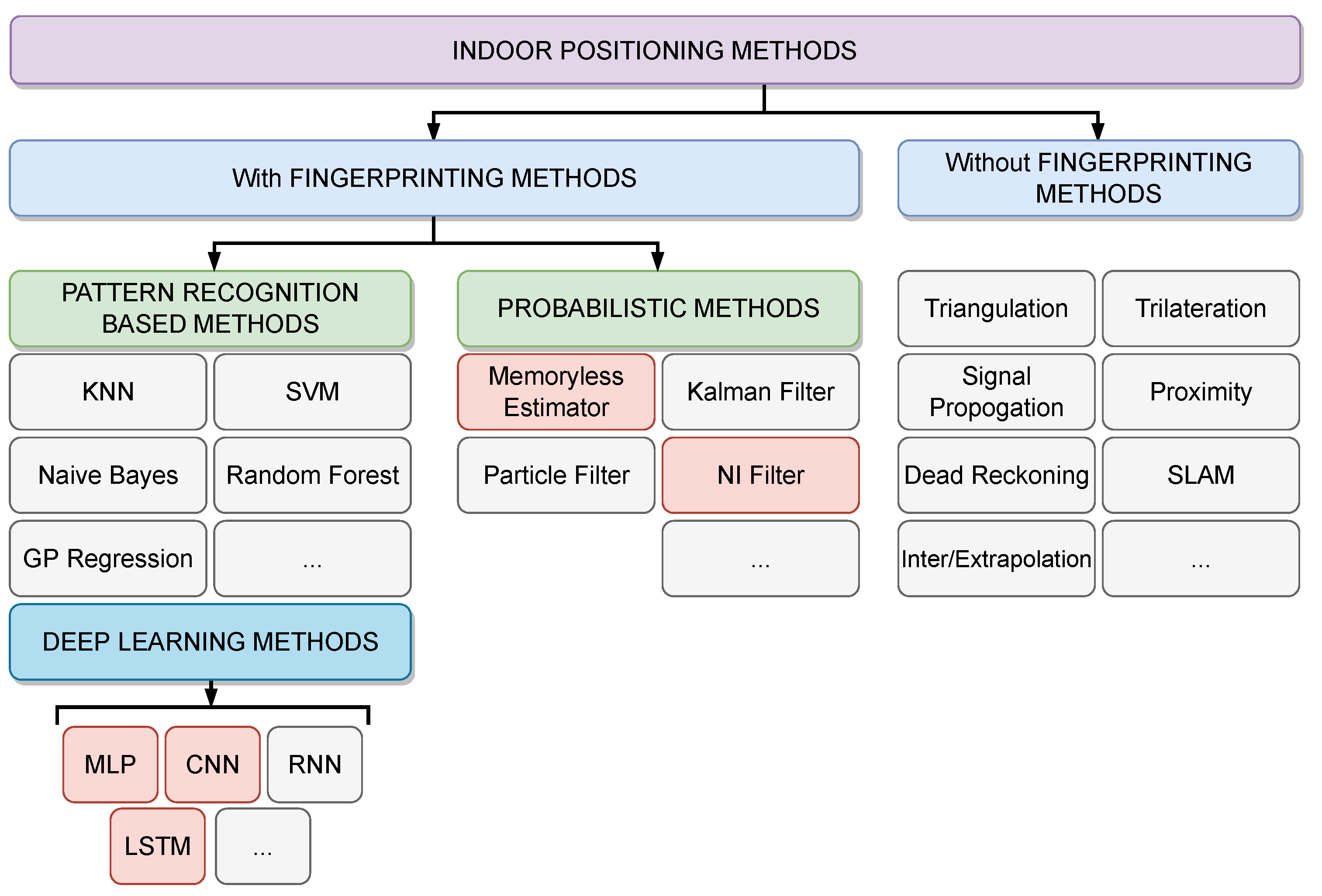
Figure 1. Classification of indoor positioning methods.
Bdcc 06 00084 g001
Figure 2. The recorded RSS Indicator data as XML format.
Bdcc 06 00084 g002
Figure 3. (a) The layout of the experimentation site with the positions of the reference points and APs (only the locations of APs on the same floor are indicated). The blue points represent the reference points from which the measurements are collected using a stationary scenario. The green points represent a novel set of reference points split for validation data. The red line is the trajectory from which the measurements are collected using a walking scenario. (b) Various numbers of APs are detected at each reference point. A total of 45 APs were detected. This number varies depending on the location. The lowest number of APs was observed at reference points around elevators, walls, and light wells in the building.
Bdcc 06 00084 g003
Figure 4. RSSI heat map or coverage map shows APs coverage ranges within the surveyed area.
Bdcc 06 00084 g004
Figure 5. Radio map. Obtained collection of fingerprint matrix layout as a result of the data preparation step of real RSS XML data measurements.
Bdcc 06 00084 g005
Figure 6. The proposed CNN and LSTM deep networks for RSS-based WLAN positioning.
Bdcc 06 00084 g006
Figure 7. Steps of building and evaluation of the proposed deep network process for RSS-based WLAN positioning.
Bdcc 06 00084 g007
Figure 8. Time-frequency transformations. (a) A sample signal, (b) Basic spectrogram using Fourier transform, (c) Constant Q transform (better resolution at low frequencies), (d) Continuous Wavelet transform (best resolution for non-periodic signals).
Bdcc 06 00084 g008
Figure 9. 1D RSS samples gathered from 45 APs and their corresponding 2D CWTs on 78 reference points. (a) 1D RSS samples gathered from 45 APs on 78 reference points. (b) corresponding 2D CWTs to 1D RSS samples on 78 reference points. (c) close-up view of RSS samples gathered at the first reference point. (d) close-up view of corresponding 2D CWTs to 1D RSS samples at the first reference point.
Bdcc 06 00084 g009
Figure 10. Two different proposed LSTM models. (a) Model 1: Lagged RSS observations as inputs. (b) Model 2: Lagged RSS observations with predicted location from the previous time step as inputs.
Bdcc 06 00084 g010
Figure 11. Two-stage HPO process. Both coarse and fine-tuning processes are used together for increased control in determining the optimum values of the hyperparameters.
Bdcc 06 00084 g011
Figure 12. Learning curve for LSTM networks Model 1 and Model 2. (a) LSTM Model 1. (b) LSTM Model 2.
Bdcc 06 00084 g012
Figure 13. Individual tracking (dynamic positioning) error results on test points. Result comparison between probabilistic models and (a) MLP deep architectures (b) 1D CNN and 2D CNN (c) LSTM Model 1 and LSTM Model 2.
Bdcc 06 00084 g013aBdcc 06 00084 g013b
Table 1. Hyperparameters with a specified range of values.
ParametersRanges [min : max : step size]
#layer size
#hidden layer
[2 : 10 : 1]
#lag time-steps[1 : 4 : 1]
#memory units[25 : 250 : 25]
#filters[8 : 64 : 8]
#neurons per hidden layer[32 : 1025 : 32]
kernel size[2 : 5 : 1]
dropout[0.1 : 0.9 : 0.1]
activation function[“elu”, “sigmoid”, “relu”, “tanh”, “selu”]
dense (FC) layer[32 : 1025 : 32]
batch size[8 : 32 : 8]
learning rate[0.1, 0.01, 0.001]
optimizers[“Adam”, “RMSprop”, “Adagrad”, “SGD”]
#epochs[10 : 50 : 10]
CWT scale length[15 : 35 : 5]
# refers to “the number of”.
Table 2. MLP, 1D CNN, and 2D CNN first stage HPO results with validation and test scores.
MLP1D CNN2D CNN
BayesianHyperbandRandomBayesianHyperbandRandomBayesianHyperbandRandom
scale length302020111202525
layer_size10731099239
dense layer
(#neurons/filters,
activation,
dropout)
(1024, E, 0.9)(416, S, 0.5)(160, Sg, 0.6)(16, S, 0.9)(56, R, 0.2)(56, R, 0.5)(32, R, 0.1)(48, R, 0.6)(56, Sg, 0.7)
(640, E, 0.1)(448, R, 0.3)(768, Sg, 0.3)(64, R, 0.4)(16, T, 0.4)(24, S, 0.4)(64, E, 0.1)(40, T, 0.2)(48, S, 0.7)
(32, Sg, 0.1)(896, E, 0.6)(352, R, 0.5)(64, E, 0.9)(48, E, 0.4)(48, S, 0.6) (56, R, 0.9)(40, E, 0.2)
(32, R, 0.4)(128, T, 0.5)(2, L)(64, E, 0.9)(48, S, 0.8)(32, T, 0.3) (24, T, 0.4)
(1024, R, 0.1)(928, T, 0.3) (64, E, 0.9)(16, S, 0.1)(56, E, 0.7) (16, R, 0.4)
(32, R, 0.1)(928, T, 0.2) (24, R, 0.9)(24, R, 0.8)(24, R, 0.6) (16, E, 0.7)
(32, R, 0.1)(448, S, 0.3) (8, R, 0.1)(32, Sg, 0.8)(24, E, 0.3) (32, E, 0.6)
(32, R, 0.1)(2, L) (8,R, 0.1)(16, T, 0.7)(56, Sg, 0.7) (8, R, 0.1)
(32, R, 0.1) (8, R, 0.1)(40, S, 0.1)(8, R, 0.1) (64, S, 0.2)
(576, R, 0.2) (8, R, 0.1)
(2, L)
dense (FC) layer (1024, E, 0.1)(416, R, 0.2)(608, S, 0.3)(32, E, 0.1)(928, E, 0.2)(640, E, 0.2)
kernel size 433433
optimizerAdamAdamAdamAdamRMSpropAdamAdamAdamAdam
learning_rate0.0010.10.10.10.10.10.0010.0010.1
batch_size82432242488816
epochs501030502030103050
val_rmse (cm)6.327.377.365.476.365.516.486.705.51
test_rmse (m)6.797.617.598.046.386.196.867.035.89
test time0.120.070.070.170.140.100.180.180.16
E, Sg, R, T, S, L is a “elu”, “sigmoid”, “relu”, “tanh”, “selu” and “linear” activation functions, respectively. # refers to “the number of”. The best scores of HPO results for each method are shown in bold.
Table 3. LSTM Model 1 and Model 2 first stage HPO results.
LSTM Model 1 (M1) and Model 2 (M2)
Bayesian Opt.HyperbandRandom Search
M1M2M1M2M1M2
lag_size313333
memory_unit17525017520020075
learning_rate0.10.10.10.010.010.01
batch_size8816241632
optimizerAdamAdamRMSRMSAdamRMS
epochs505020302040
val_rmse (cm)0.130.100.140.120.130.11
test_rmse (m)4.874.085.044.664.734.23
RMS is RMSprob optimizer.
Table 4. MLP, 1D CNN, and 2D CNN second stage Grid Search results.
Parameters’ Sets Based on
First Stage Tuning Results
Grid Search
Optimal Hyperparameters
MLP1D CNN2D CNN
#hidden layer
#convolutional layer
[3, 7]
[9]
399
#filter[56, 64]-5664
#neurons per hidden layer[640, 1024](1 × 1024, 2 × 640)--
kernel size[3]-33 × 3
dropout (MLP)
dropout (CNNs)
[0.1]
[0.4]
0.10.40.4
activation function (MLP)
activation function (CNNs)
[“elu”, “relu”, “sigmoid”]
[“elu”, “relu”, “selu”]
“relu”“selu”“elu”
#neurons of dense layer[608, 640, 720]-608720
batch size[8, 16]1688
learning rate[0.1, 0.01, 0.001]0.10.0010.001
optimizerAdamAdamAdamAdam
epochs (MLP)
epochs (CNNs)
[30, 40, 50]
[30, 50]
403050
CWT scale parameter (MLP)
CWT scale parameter (2D CNN)
[20, 25, 30]
[25, 30]
20130
val_rmse (cm) 4.80 ± 0.35.72 ± 0.144.51 ± 0.89
test_rmse (m) 5.30 ± 0.025.39 ± 0.195.30 ± 0.44
# refers to “the number of”.
Table 5. LSTM Model 1 and Model 2 second stage Grid Search results.
LSTMModel 1Model 2
Parameters’ Sets Based on
First Stage Tuning Results
Fine Tuning (Grid Search)
Optimal Hyperparameters
lag_size[2, 3, 4]44
memory_unit[175, 200]175175
learning_rate[0.1, 0.01]0.010.01
batch_size[8, 16, 32]88
optimizer[“Adam”, “RMSprop”]AdamAdam
epochs[20, 30, 50]2020
val_rmse (cm) 0.09 ± 0.070.07 ± 0.06
test_rmse (m) 2.78 ± 0.041.73 ± 0.06
Table 6. Dynamic positioning error statistics for different models.
MLP1D CNN2D CNNLSTM
Model 1
LSTM
Model 2
Memoryless
Estimator
NI Constant
Velocity
NI Constant
Acceleration
NI Variable
Acceleration
Training time (s) (mean ± std)5.55 ± 0.2827.91 ± 0.46818.24 ± 4.001.36 ± 1.041.61 ± 1.48
Test time (s)0.080.120.380.050.05
Total number of parameters1,861,5061,466,11413,983,986281,052288,052
RMSE (m) (mean ± std)5.30 ± 0.025.39 ± 0.195.30 ± 0.442.78 ± 0.041.73 ± 0.0610.356.55.335.2
Publisher’s Note: MDPI stays neutral with regard to jurisdictional claims in published maps and institutional affiliations.