A Non-Uniform Continuous Cellular Automata for Analyzing and Predicting the Spreading Patterns of COVID-19

Abstract

During the COVID-19 outbreak, modeling the spread of infectious diseases became a challenging research topic due to its rapid spread and high mortality rate. The main objective of a standard epidemiological model is to estimate the number of infected, suspected, and recovered from the illness by mathematical modeling. This model does not capture how the disease transmits between neighboring regions through interaction. A more general framework such as Cellular Automata (CA) is required to accommodate a more complex spatial interaction within the epidemiological model. The critical issue of modeling in the spread of diseases is how to reduce the prediction error. This research aims to formulate the influence of the interaction of a neighborhood on the spreading pattern of COVID-19 using a neighborhood frame model in a Cellular-Automata (CA) approach and obtain a predictive model for the COVID-19 spread with the error reduction to improve the model. We propose a non-uniform continuous CA (N-CCA) as our contribution to demonstrate the influence of interactions on the spread of COVID-19. The model has succeeded in demonstrating the influence of the interaction between regions on the COVID-19 spread, as represented by the coefficients obtained. These coefficients result from multiple regression models. The coefficient obtained represents the population’s behavior interacting with its neighborhood in a cell and influences the number of cases that occur the next day. The evaluation of the N-CCA model is conducted by root mean square error (RMSE) for the difference in the number of cases between prediction and real cases per cell in each region. This study demonstrates that this approach improves the prediction of accuracy for 14 days in the future using data points from the past 42 days, compared to a baseline model.

1. Introduction

The Coronavirus disease (COVID-19) was first reported in China at the end of 2019 [1,2,3]. The rapid spread of this disease encouraged researchers to develop epidemiological models for the spread of this disease. Such models are useful for understanding the transmission patterns of the disease, which in turn, help us in formulating optimal strategies to curb the spread and lessen the impact of the outbreak [4,5].

The main objective of a standard epidemiological model is to estimate, at a certain time point, the number of individuals who are infected by the disease, suspected to have been infected, recovered from the illness, etc. We can model these quantities of interest, called compartment, deterministically or stochastically, i.e., as random variables. In the case of COVID-19, one category of approaches formulates the relationships between those quantities explicitly as a set of differential equations, which are then solved analytically, numerically, or through simulations. Depending on which compartments were being considered, these led to the SIR [6,7,8], SEIR [9,10,11], SLIR [12,13,14], SIRD [15,16], SEIRU [17], SLIAR [12], and SIDARTHE [18,19] models. Meanwhile, another category of approaches employs machine learning models to capture the relationships between those compartments [20,21]. Such models are trained using data, which may be available as a time series. Some researchers even use news and social media data to model the trends in the growth of COVID-19 cases [4].

Although these models can provide estimates of the compartments, they do not capture how the disease can be transmitted between neighboring regions through the movement of individuals between them. As a result, such estimates tend to be inaccurate. In fact, a study by Anirudh [22] pointed out that the error estimate of such models ranges between 13% and 225%. One contributing factor is the lack of spatial elements in the models, and Bohner et al. [23] argued that such spatial elements need to be incorporated to obtain a better model.

Traditional approaches for such spatially aware epidemiological models use a set of partial differential equations (PDEs) where each compartment variable is not only time-dependent but also spatial-dependent, as described by Murray [24]. Therein, the spatial interaction is represented by a diffusion coefficient that indicates the dispersion rate of the disease along the spatial dimensions, and the resulting PDEs include the rate of changes with respect to both temporal and spatial dimension. A more fine-grained metapopulation model (also known as the patch occupancy model) for the epidemiological model is proposed by Arino et al. [25], who introduce spatial patches, which correspond to regions in space, allowing a more explicit modeling of interaction between different regions in the epidemiological model. Instead of PDEs, Arino et al. uses ordinary differential equations (ODEs) and demonstrates the simulation of the model only in the case of one-way and two-way migration between neighboring regions that form a ring structure topologically—each region has only two neighbors on its “left” and “right”.

To accommodate a more complex spatial interaction within the epidemiological model, a more general framework is needed [26]. To this end, we turn to cellular automata [27]. Cellular automata (CA) is a dynamic system that is defined over a d-dimensional lattice of cells. At each time step, a cell has a value that corresponds to one of the possible states. In its most basic form, there are only finitely many possible such states for each cell. However, it is possible to consider an infinite, or even uncountable, set of states. Interaction between a cell with another cell in its neighborhood is expressed in terms of transition rules that determine how the cell’s state can change due to that interaction. When a CA is simulated by running it for a certain number of time steps, we can capture a variety of spatiotemporal dynamics of the states. Unsurprisingly, this characteristic is appropriate for epidemiological models whose aim is to represent the spreading behavior of infectious diseases particularly during an outbreak, which is spatiotemporal in nature [28,29,30,31,32,33,34].

When using CA for modeling disease outbreaks, we usually restrict our attention to a particular region as a scope in which the CA operates, e.g., a country, a district, or even a residential area. The CA cells are defined over such a region, and a straightforward way to represent dynamics in epidemiological modeling is to associate each cell’s state to the condition of one individual with respect to the disease being modeled, e.g., exposure, infection, recovery, etc. That is, the set of states of the CA is discrete. Here, each cell implicitly corresponds to a single individual only, and the transition rules govern how the disease can be transmitted from one individual to another. Simulating such local interactions between individuals in the population over a time period can lead to interesting patterns that can be analyzed at the global level [35]. This approach differs from metapopulation models such as that from Arino et al. [25], which allows only global interactions between spatial patches.

In the case of COVID-19, epidemiological models based on CA have been proposed by a number of researchers [36,37,38,39,40]. All of them employ the so-called probabilistic CA, where the transition rules are probabilistically defined as a discrete set of states, as described earlier. These probabilistic CAs are also uniform in nature in the sense that the same probabilistic transition rules are applied to all cells.

The usage of these CA models for modeling the spread of COVID-19 follows a rather typical simulation-based approach. Specifically, such a CA model would have a fixed set of transition rules, which governs both the movement of individuals from one cell to another as well as the epidemiological dynamics due to disease transmission, mortality, and other related factors. To predict the size of the compartments, e.g., the number of infected individuals, at the nth time step, we would start with an initial state with parameters initialized from data and background knowledge about the disease. Then, we run a simulation on the CA by executing transition rules at each time step until reaching the nth time step. At the end of the simulation, a comparison could be made for predictions of solutions to the standard epidemiological modeling based on differential equations. However, such a comparison was not performed by all of the CA-based epidemiological models, except by Ghosh and Bhattacharya [37], who reported a prediction accuracy in the range of 65–75% at the peak of the epidemic. Note that in all cases, the performance depends in principal on the initial parameter setting prior to simulation. Hence, we need to conduct a trial-and-error approach to obtain an optimal setting.

Our aim in this paper is to come up with a way to reduce a prediction error using CA-based modeling. Such an error can be caused by a number of unaccounted factors in the model such as complex interactions between neighboring regions due to movements of individuals in the population, the differing characteristics of crowds at different locations, level of vaccination in the population, or the prevalence of comorbidities. Among these factors, we focus on the influence of imperceptible interactions between neighboring regions that may influence disease spread in the epidemiological modeling for better modeling by proposing a way to represent them that improves the predictive power of CA-based models.

More precisely, we start from a sequence of data points $I_0,I_1,\dots ,I_k$ of compartment variable values obtained from real-world data, e.g., the number of infected individuals over consecutive days. Then, we generate a sequence $M_1,M_2,\dots ,M_k$ where each $M_i$ is the prediction for the value of $I_i$ obtained by solving the standard mathematical model of epidemiology such as the SIRD model using the value of $I_{i-1}$ and the known epidemiological model parameters at the $(i-1)$th time step (transmission rate, mortality rate, and incubation period). In our case, the transmission rate follows that of Viceconte [41]. The incubation period and mortality rate follow that of Li et al. [2]. The difference between $M_i$ and $I_i$ constitutes an error due to unaccounted interactions between regions. We then formulate a multiple regression model to estimate for each cell the influence of each of its neighboring cells on the prediction. Here, instead of explicitly including movements of individuals as part of the model, we abstract them away as influence measures between neighboring regions. Once these influence measures are estimated, we can use them to predict the state of the epidemiological variable at the nth time step with $n>k$ by running a simulation on a CA initialized with parameters from data at the kth time step.

Note that the CA we employ is continuous because the states of the CA can contain real numbers during simulation [42]. That is, the simulation essentially computes $M_{k+1}$ up to $M_n$ where for $i>k$, $M_i$ depends on the value of $M_{i-1}$ (except $M_{k+1}$ that depends on $I_k$). Here, $M_i$ need not be an integer, and moreover, it is not estimated based on $I_i$, which is not present when $i>k$. Obviously, at the nth time step, the predicted value of the considered compartment variable may need to be rounded to an integer if we wish to obtain an actual count. Note that this is in contrast to the existing CA-based models for the COVID-19 spread, where the states correspond to single individuals and thus have discrete values.

It is also non-uniform because the transition rules are different among different cells [30]. The differences are due to the fact that the states of the CA are continuous and the transition rules for each cell depend on the influence measure from its neighbors, which may be different. In addition, in our CA model, each cell explicitly refers to an actual subregion part of the considered region (e.g., an area in a province of a country).

Overall our contribution is as follows. First, we propose a way to represent the influence between neighboring regions in COVID-19 epidemiological modeling that abstracts away from explicit inclusion of movement of individuals employed by existing CA-based models. It shows that a CA-based approach can be applied without requiring explicit individual movement. These influence measures are estimated via multiple regression models making use of the difference between compartment variable values according to the actual data and those values according to the standard epidemiological model. Second, we propose the use of non-uniform continuous CA (N-CCA) as a prediction engine through simulation where the initial parameters take into account the aforementioned influence measures between neighboring regions. We then demonstrate that this approach improves the prediction of accuracy on the number of infected individuals up to 14 days in the future using data points from the past 42 days, compared to a baseline model from Fong et al. [43]. This baseline model uses a composite Monte-Carlo simulation to forecast the overall trend and propagation of the infected cases during the early period of the epidemic in China. The simulation is enhanced by a deep learning network and fuzzy rule induction applied to limited data and takes into account the spatiotemporal influence of nearby cities. In their evaluation, a 14-day forecast is created for all of China, and the result yields an RMSE of about 62,077.26.

This paper is organized as follows. After the introduction in this section, Section 2 details relevant related works. Section 3 provides a more formal definition of CA employed in our model. In addition, in this section, we describe the detailed formulation of our model and the data set used to build it. The simulation and prediction results are presented in Section 4, followed by a discussion of the results in Section 5. In Section 6, we present the conclusion of our research and suggestions for future works.

2. Related Works

Our study compares the baseline model from Fong et al. [43] that used a Composite Monte Carlo method simulation, enhanced by a deep learning network and fuzzy rule induction applied to limited data [43]. Fong et al. [43] proposed a new Monte Carlo model called the Composite Monte Carlo model (CMCM), which accepts predictor variables from multi-pronged data sources that correlate with each other. The baseline model forecasts the overall trend and propagation of the infected cases during the early epidemic in China, influenced by the temporal-spatial data of the nearby cities around Wuhan. The experiment uses some data, namely data on the number of people in China who have contracted the COVID-19 disease. The evaluation results give an RMSE of 62,077.26.

Several studies related to using the CA method for modeling the spread of COVID-19 are still infrequent and only appeared in mid-2020. The researchers are still focused on simulations. Intending to prove the sensitivity of the CA model, Dascǎlu et al. [36] carried out simulations with occlusion in the cellular space and performed them probabilistically for individual movement within cells as a defined transition function. Other researchers simulated data of forty countries from different continents by constructing a 100 × 100 cellular space simulation for each country that scaled to population density. Next, they applied a probabilistic CA with a genetic algorithm as a transition function [37]. Other studies used probabilistic CA in a cellular space measuring 400 × 400. This study involved population density factors and the efficiency of the COVID-19 test in self-isolation [39]. This simulation used 100,000 populations that were placed randomly in the cellular space. They tried different probability values for the density and the isolation factors as the transition function.

A similar study used the CA probabilistic method in conducting simulations on a 210 × 210 cellular space [38]. They carried out a simulation using five neighborhoods with population data from Brazil, which equated to around 250,000 individuals, and included isolation factors for the simulation. They defined a transition function that was composed of probabilities. They also randomly assigned the initial states. Another simulation using case data in New York and Iowa used probabilistic CA [40]. The simulation model includes isolation and diagnostic factors. They proportionally adjusted probabilistic treatment values to see the peak and the end of the pandemic with the aim tof developing a strategy to control the spread of cases.

3. Materials and Methods

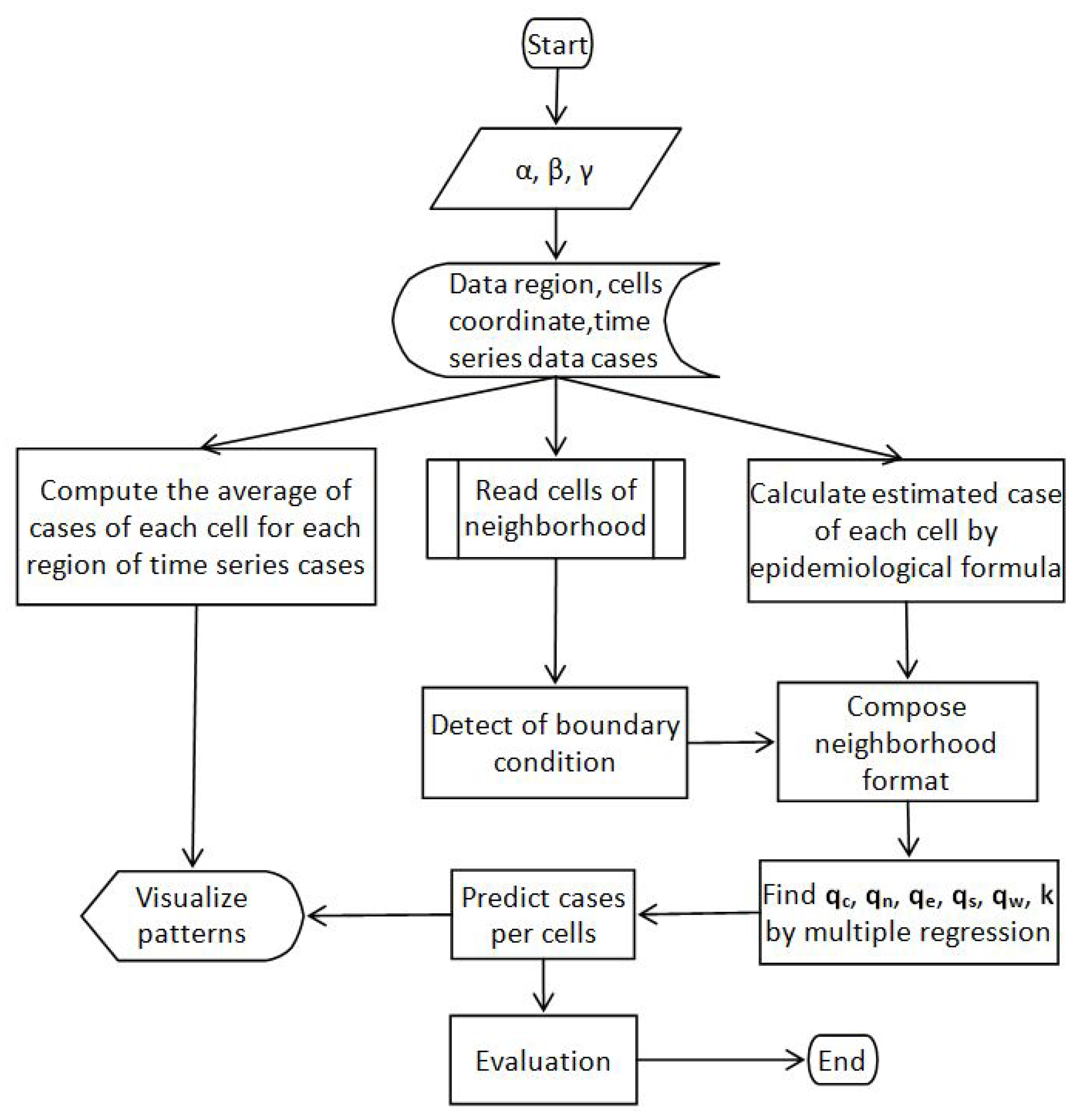
Our overall workflow is shown in Figure 1. To start the process, we took the values of the three epidemiological parameters, $\alpha$, $\beta$, and $\gamma$, for China from a pre-existing study and input them into the model. The model reads data from input tables consisting of region data, cell coordinate data, and time-series data cases.

In the next step, we simultaneously carried out a process for: computing the average cases of each cell for each region of time series cases, reading cells of neighborhood data, and calculating estimated cases, adding each cell with an epidemiological formula. In the next step, we compose a time series of cases in neighboring format for each cell by boundary detection. In the next block, we find the values of $q_c$, $q_n$, $q_e$, $q_s$, $q_w$, and k for each cell using multiple regression and use it to predict cases for the next few days on the next block. In the last block, the prediction results are evaluated and displayed.

3.1. Cellular Automata

A cellular automaton (CA) is a 4-tuple $(C,S,V,f)$ where $C\subseteq {\left({\mathbb{Z}}^{+}\right)}^D$ is simply a set of D-tuples of positive integers called a cellular space [28]. Elements of C are called cells. A cellular space is typically arranged as a d-dimensional grid following a coordinate system based on matrix-indexing convention where the D-tuple containing all ones, $(1,\dots ,1)$ lies on the origin position of the grid (i.e., the top-left corner in a 2-dimensional grid), and the cell $c=(x_1,\dots ,x_D)$ borders with $2D$ other cells (except when c is at the edge of the grid). For example, in 2-dimensional grid, cell $(i,j)$ borders with $(i-1,j)$ at the top, with $(i,j+1)$ to the right, with $(i,j+1)$ at the bottom, and with $(i,j-1)$ to the left [27,44,45].

$S$ is a set of states for each cell, which encapsulates all possible conditions a cell may be in. Depending on the nature of the problem to be modeled, $S$ may consist of discrete scalar values, continuous scalar values, or even tuples of such values. A CA is continuous if $S$ is continuous. Otherwise, the CA is discrete, which is how CA is traditionally defined.

$V:{\left({\mathbb{Z}}^{+}\right)}^D\to 2^{{\left({\mathbb{Z}}^{+}\right)}^D}$ defines the neighborhood frame $V\left(c\right)=\{c,v_1\left(c\right),\dots ,v_m\left(c\right)\}$ of a cell c. Here, m is fixed and each $v_i:{\left({\mathbb{Z}}^{+}\right)}^D\to {\left({\mathbb{Z}}^{+}\right)}^D$ is a fixed function returning a neighbor cell of the given cell c. Thus, c can have up to m neighbors in the model and each of those neighbors contributes to the dynamics of c when the CA is simulated.

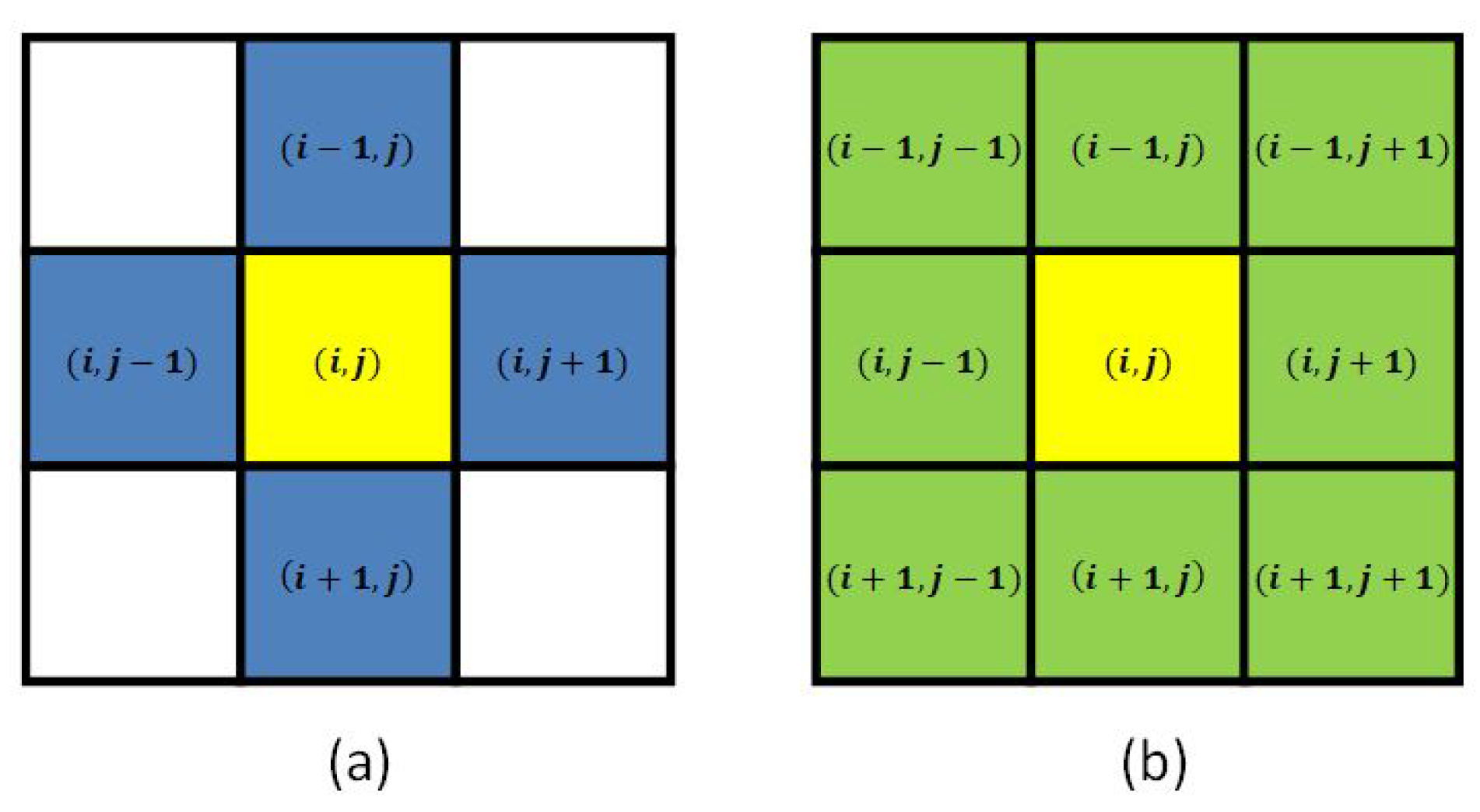
Two of the most commonly used neighborhood frames are von Neumann neighborhood and Moore neighborhood [29,30]. Von Neumann neighborhood with radius $r\in \mathbb{N}$ of a cell c consists of cells with a Manhattan distance of at most r from c. Meanwhile, a Moore neighborhood with radius $r\in \mathbb{N}$ of a cell c consists of cells with a Chebyshev distance of at most r from c. (A Manhattan distance of $\mathit{u}=(u_1,\dots ,u_d)$ and $\mathit{w}=(w_1,\dots ,w_d)$ is ${\sum }_i\left|u_i-w_i\right|$, while their Chebyshev distance is ${max}_i\left|u_i-w_i\right|$). Note that the indices for such neighborhood frames follow the matrix-index convention when, i.e., for cells $(i,j)$ in a 2D cellular space, i increases from “top” to “bottom”, while j increases from “left” to “right”. Figure 2 illustrates Von Neumann and Moore neighborhood frames in the 2-dimensional cellular space. The Von Neumann neighborhood of $c=(i,j)$ with radius 1 is $\left\{\right(i,j),(i-1,j),(i,j+1),(i+1,j),(i,j-1\left)\right\}$. Meanwhile, the Moore neighborhood of $c=(i,j)$ with radius 1 is $\left\{\right(i,j),(i-1,j),(i-1,j+1),(i,j+1),(i+1,j+1),(i+1,j),(i+1,j-1),(i,j-1),(i-1,j-1\left)\right\}$.

Next, $f:S^{m+1}\to S$ is a local transition function that governs how the new state of a cell is obtained from the old state of that cell and the states of that cell’s neighbors [28]. Therefore, if $s_c,s_{v_1\left(c\right)},\dots ,s_{v_m\left(c\right)}$ are the current state of a cell c and its neighbors, then $s_c^{\prime }=f(s_c,s_{v_1\left(c\right)},\dots ,s_{v_m\left(c\right)})$ is the new state of the cell c. A CA is traditionally uniform in the sense that f has the same definition across all cells. However, in this paper, we allow f to be different across different cells, i.e., the CA to be non-uniform.

The simulation of a CA can be understood as a sequence of applications of the local transition function on the state of all cells at consecutive time steps. Therefore, we use $s_c^t$ to denote the state of a cell c at time step t. Then, a configuration $S_t$ at time step t is the set $\{s_c^t\mid c\in C\}$. A one-step simulation of the CA is a function G that returns $S_{t+1}$ given $S_t$ defined as $S_{t+1}=G\left(S_t\right)=\{f(s_c^t,s_{v_1\left(c\right)}^t,\dots ,s_{v_m\left(c\right)}^t)\mid c\in C\}$. Finally, a simulation of the CA starting from an initial configuration $S_0$ is simply an iterative application of G denoted by $S_0\mapsto G\left(S_0\right)\mapsto G^2\left(S_0\right)\mapsto \dots$. Therefore, obviously $G^k\left(S_0\right)$ corresponds to k steps of simulation of the CA starting from $S_0$.

3.2. SIRD Epidemiological Model

Here, we introduce the SIRD model as the underlying mathematical model of the spread of infectious diseases based on the formulation by Siettos and Russo [46], Nepomuceno et al. [47]. The SIRD model is a variant of the basic SIR model where at any given time, we consider the population (in which the disease spreads) partitioned into four disjoint subsets or compartments, namely the susceptibles (S), the infected (I), the recovered (R), and the deaths (D). The relationships between these compartments can be expressed by the following system of ordinary differential equations (ODEs) where $\alpha$ denotes the mortality rate among the infected, $\beta$ denotes the transmission rate among the infected, i.e., how many healthy individuals can become infected per unit time by an already infected individual, and $1/\gamma$ denotes the incubation period, i.e., the duration in which the disease remains infectious—beyond this period, one assumes that an infected individual no longer spreads the disease to others.

$$\begin{array}{cc}\hfill \frac{dS}{dt}& =-\beta I\hfill \end{array}$$

(1)

$$\begin{array}{cc}\hfill \frac{dI}{dt}& =\beta I-\gamma I-\alpha I\hfill \end{array}$$

(2)

$$\begin{array}{cc}\hfill \frac{dR}{dt}& =\gamma I\hfill \end{array}$$

(3)

$$\begin{array}{cc}\hfill \frac{dD}{dt}& =\alpha I\hfill \end{array}$$

(4)

The variables $S,I,R$, and D are time-dependent and the parameters $\alpha ,\beta$, and $\gamma$ are specified in terms of a particular time unit. Intuitively, Equation (1) states that the size of the susceptibles at a given time decreases due to a proportion of it becoming infected. Equation (2) expresses the change in the size of the infected due to the addition of newly infected individuals as well as the removal of individuals due to fatalities as well as those who have passed the incubation period. Equation (3) describes the addition to the recovered by individuals who are no longer infectious, while Equation (4) expresses that a proportion of the infected do not survive and is thus added to the death compartment.

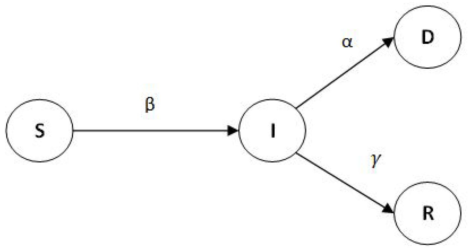
Note that $S,I,R$, and D can also be viewed as states in which an individual in the population can belong. The relationships between them can also be illustrated as a state diagram as in Figure 3.

Given the epidemiology model parameters $\alpha ,\beta$, and $\gamma$, we can solve the ODE system to obtain an explicit form of $S,I,R$, and D as a function of time. A comparison of data can then be made to see if the parameter setting is appropriate. If the parameters are unknown, the estimation can be performed via various approaches of nonlinear regression [48]. However, note that this formulation does not take into account the spatial aspect of the disease spread. Our next aim is to accommodate this using a CA-based model, specifically to estimate the number of infected at a given time step t. We apply our model to the spread of disease. In this matter, we limit our scope only to the infected compartment and focus our attention on Equation (2).

3.3. Proposed CA-Based SIRD Epidemiological Model

In our CA-based approach, we work on cells in a fixed finite 2-dimensional grid that forms a cellular space. Each of these cells maintains a variable $I_{i,j}^t$ that represents the number of infected in cell $(i,j)$ at time step t. Here, each cell should be viewed as a representation of an actual spatial region in which a number of infected/susceptible/healthy individuals may reside. Since the CA configuration has discrete characteristics, we could change Equation (2) into discrete form. Discretizing Equation (2), we obtain the following relation:

$$I_{i,j}^t-I_{i,j}^{t-1}=\beta I_{i,j}^{t-1}-\gamma I_{i,j}^{t-1}-\alpha I_{i,j}^{t-1}+\delta$$

(5)

The left-hand side of Equation (5) expresses the change of $I_{i,j}$ between consecutive time steps according to the real data, while the right-hand side (except the $\delta$ term) represents the approximation of that change according to the SIRD epidemiological model. The $\delta$ term corresponds to the discrepancy between the two. Our idea is to model $\delta$ as the result of the interaction between cell $(i,j)$ and its neighbors that contributes to the change in the number of infected in cell $(i,j)$. Concretely, infected individuals from a neighboring cell can cause the disease to spread to individuals in cell $(i,j)$. This is represented by an interaction coefficient q specific for that neighboring cell. Specifically, if a cell $(i,j)$ has m neighbors, then there are $m+1$ different coefficients that determine the current level of infection $(i,j)$ as well as at its neighboring cells added to the future level of infection at $(i,j)$.

To simplify our discussion, we focus on the Von Neumann neighborhood with radius 1 for the CA-based approach in this paper. Thus, a cell $(i,j)$ has four neighboring cells, namely the “north” cell $(i-1,j)$, the “east” cell $(i,j+1)$, the “south” cell $(i+1,j)$, and the “west” cell $(i,j-1)$. The interaction coefficients for those neighboring cells are, respectively, $q_n,q_e,q_s$, and $q_w$. In addition, $q_c$ represents the inner interaction coefficient of the “center” cell, i.e., cell $(i,j)$ to itself. 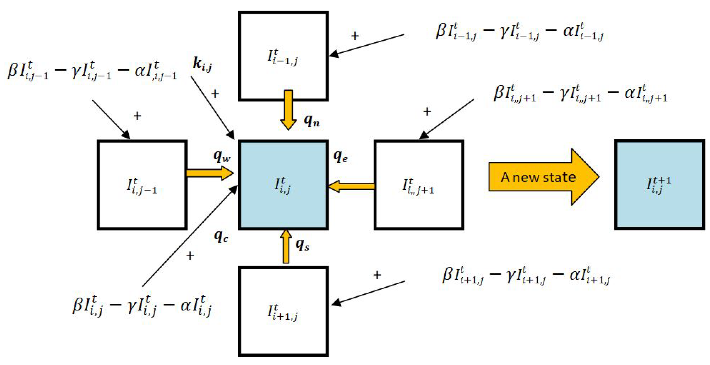Note that all these interaction coefficients are dependent on $(i,j)$, i.e., their values are different when a different “center” cell is considered. Hence, as illustrated in Figure 4, we can rewrite Equation (5) into Equation (6):

$$I_{i,j}^t-I_{i,j}^{t-1}=q_{c,i,j}{P}_{c,i,j}^{t-1}+q_{n,i,j}{P}_{n,i,j}^{t-1}+q_e{P}_{e,i,j}^{t-1}+q_{s,i,j}{P}_{s,i,j}^{t-1}+q_{w,i,j}{P}_{w,i,j}^{t-1}+k_{i,j}$$

(6)

where $k_{i,j}$ is a bias or offset term, while $P_{c,i,j}^{t-1},P_{n,i,j}^{t-1},P_{e,i,j}^{t-1},P_{s,i,j}^{t-1}$, and $P_{w,i,j}^{t-1}$ are the estimated number of additional infected individuals in each cell $c^{\prime }\in V(i,j)$, the neighborhood frame of cell $(i,j)$, which are expressed as Equation (7) below.

$$\begin{array}{cc}\hfill P_{c,i,j}^{t-1}& =\beta I_{i,j}^{t-1}-\gamma I_{i,j}^{t-1}-\alpha I_{i,j}^{t-1}\hfill \\ \hfill P_{n,i,j}^{t-1}& =\beta I_{i,j+1}^{t-1}-\gamma I_{i,j+1}^{t-1}-\alpha I_{i,j+1}^{t-1}\hfill \\ \hfill P_{e,i,j}^{t-1}& =\beta I_{i+1,j}^{t-1}-\gamma I_{i+1,j}^{t-1}-\alpha I_{i+1,j}^{t-1}\hfill \\ \hfill P_{s,i,j}^{t-1}& =\beta I_{i,j-1}^{t-1}-\gamma I_{i,j-1}^{t-1}-\alpha I_{i,j1}^{t-1}\hfill \\ \hfill P_{w,i,j}^{t-1}& =\beta I_{i-1,j}^{t-1}-\gamma I_{i-1,j}^{t-1}-\alpha I_{i-1,j}^{t-1}\hfill \end{array}$$

(7)

As stated in the introduction as well as Figure 1, we work with a time series data representing the number of infected individuals during a certain period of time. Therefore, we have data points for each cell $(i,j)$ as a sequence of values $I_{i,j}^0,I_{i,j}^1,\dots ,I_{i,j}^N$, each representing the number of infected individuals in cell $(i,j)$ at time step $t=0,\dots ,N$. Based on these data, Equation (6) yields the following system of N linear equations for cell $(i,j)$ in Equation (8) (with subscript $(i,j)$ omitted for P’s and q’s).

$$\begin{array}{cc}\hfill I_{i,j}^1-I_{i,j}^0& =k_{i,j}+q_c{P}_c^0+q_n{P}_n^0+q_e{P}_e^0+q_s{P}_s^0+q_w{P}_w^0\hfill \\ \hfill I_{i,j}^2-I_{i,j}^1& =k_{i,j}+q_c{P}_c^1+q_n{P}_n^1+q_e{P}_e^1+q_s{P}_s^1+q_w{P}_w^1\hfill \\ \hfill & ⋮\hfill \\ \hfill I_{i,j}^N-I_{i,j}^{N-1}& =k_{i,j}+q_c{P}_c^{N-1}+q_n{P}_n^{N-1}+q_e{P}_e^{N-1}+q_s{P}_s^{n-1}+q_w{P}_w^{N-1}\hfill \end{array}$$

(8)

The above system can be expressed in a matrix form (Equation (9)) for each cell $(i,j)$:

$$\Delta {\mathit{I}}_{i,j}={\mathit{P}}_{i,j}{\mathit{q}}_{i,j}$$

(9)

where

• $\Delta {\mathit{I}}_{i,j}={[\Delta I_{i,j}^1,\dots ,\Delta I_{i,j}^N]}^{\mathsf{T}}$ is an N-dimensional vector whose tth element ($t=1,\dots ,N$) is $\Delta I_{i,j}^t=I_{i.j}^t-I_{i,j}^{t-1}$ for each $t=1,\dots ,N$,
• ${\mathit{P}}_{i,j}$ is an $N\times 6$ matrix whose t’th row is the vector ${[1,P_c^{t-1},P_n^{t-1},P_e^{t-1},P_s^{t-1},P_w^{t-1}]}^{\mathsf{T}}$
• ${\mathit{q}}_{i,j}$ is a 6-dimensional vector ${[k_{i,j},q_c,q_n,q_e,q_s,q_w]}^{\mathsf{T}}$ with $t=1,\dots ,N$.

Our aim is to find the values of ${\mathit{q}}_{i,j}$ for all cells $(i,j)$ such that the changes on the number of infected individuals at time t predicted by accounting for the neighboring cell interactions as represented by ${\mathit{P}}_{i,j}$ accurately approximates the changes of the number of infected individuals in the actual data as represented by $\Delta {\mathit{I}}_{i,j}$. Therefore, we view this as a multiple linear regression problem where we optimize ${\mathit{q}}_{i,j}$.

More precisely, let $J\left(\mathit{q}\right)$ be a sum-of-squares loss function (expressed using L2 vector norm) for the aforementioned regression problem where we omit the subscript $(i,j)$:

$$\begin{array}{cc}\hfill J\left(\mathit{q}\right)& ={\parallel \Delta \mathit{I}-\mathit{P}\mathit{q}\parallel }^2={(\Delta \mathit{I}-\mathit{P}\mathit{q})}^{\mathsf{T}}(\Delta \mathit{I}-\mathit{P}\mathit{q})=(\Delta {\mathit{I}}^{\mathsf{T}}-{\left(\mathit{P}\mathit{q}\right)}^{\mathsf{T}})(\Delta \mathit{I}-\mathit{P}\mathit{q})\hfill \\ \hfill & =\Delta {\mathit{I}}^{\mathsf{T}}\Delta \mathit{I}-{\left(\mathit{P}\mathit{q}\right)}^{\mathsf{T}}\Delta \mathit{I}-\Delta {\mathit{I}}^{\mathsf{T}}\mathit{P}\mathit{q}+{\left(\mathit{P}\mathit{q}\right)}^{\mathsf{T}}\mathit{P}\mathit{q}\hfill \end{array}$$

(10)

Examining the shape of the matrices and vectors above, we notice that both ${\left(\mathit{P}\mathit{q}\right)}^{\mathsf{T}}\Delta \mathit{I}$ and $\Delta {\mathit{I}}^{\mathsf{T}}\mathit{P}\mathit{q}$ are scalars. Therefore, ${\left(\mathit{P}\mathit{q}\right)}^{\mathsf{T}}\Delta \mathit{I}={({\left(\mathit{P}\mathit{q}\right)}^{\mathsf{T}}\Delta \mathit{I})}^{\mathsf{T}}=\Delta {\mathit{I}}^{\mathsf{T}}\mathit{P}\mathit{q}$. Thus, Equation (10) becomes Equation (11):

$$\begin{array}{cc}\hfill J\left(\mathit{q}\right)& =\Delta {\mathit{I}}^{\mathsf{T}}\Delta \mathit{I}-2\Delta {\mathit{I}}^{\mathsf{T}}\mathit{P}\mathit{q}+{\left(\mathit{P}\mathit{q}\right)}^{\mathsf{T}}\mathit{P}\mathit{q}=\Delta {\mathit{I}}^{\mathsf{T}}\Delta \mathit{I}-2\Delta {\mathit{I}}^{\mathsf{T}}\mathit{P}\mathit{q}+{\mathit{q}}^{\mathsf{T}}{\mathit{P}}^{\mathsf{T}}\mathit{P}\mathit{q}\hfill \end{array}$$

(11)

Therefore, finding an optimal $\mathit{q}$ means we need to solve the following optimization problem in Equation (12):

$$\widehat{\mathit{q}}=\underset{\mathit{q}}{argmin}J\left(\mathit{q}\right)=\underset{\mathit{q}}{argmin}[\Delta {\mathit{I}}^{\mathsf{T}}\Delta \mathit{I}-2\Delta {\mathit{I}}^{\mathsf{T}}\mathit{P}\mathit{q}+{\mathit{q}}^{\mathsf{T}}{\mathit{P}}^{\mathsf{T}}\mathit{P}\mathit{q}]$$

(12)

The gradient of the loss function is ${\nabla }_{\mathit{q}}J\left(\mathit{q}\right)$, defined in Equation (13):

$$\begin{array}{cc}\hfill {\nabla }_{\mathit{q}}J\left(\mathit{q}\right)& ={\nabla }_{\mathit{q}}(\Delta {\mathit{I}}^{\mathsf{T}}\Delta \mathit{I}-2\Delta {\mathit{I}}^{\mathsf{T}}\mathit{P}\mathit{q}+{\mathit{q}}^{\mathsf{T}}{\mathit{P}}^{\mathsf{T}}\mathit{P}\mathit{q})\hfill \\ \hfill & =0-2{(\Delta {\mathit{I}}^{\mathsf{T}}\mathit{P})}^{\mathsf{T}}+\left({\mathit{P}}^{\mathsf{T}}\mathit{P}\right)\mathit{q}+{\left({\mathit{P}}^{\mathsf{T}}\mathit{P}\right)}^{\mathsf{T}}\mathit{q}\hfill \\ \hfill & =-2{\mathit{P}}^{\mathsf{T}}\Delta \mathit{I}+2{\mathit{P}}^{\mathsf{T}}\mathit{P}\mathit{q}\hfill \end{array}$$

(13)

Setting ${\nabla }_{\mathit{q}}J\left(\mathit{q}\right)=0$ yields Equation (14):

$$\begin{array}{c}\hfill {\mathit{P}}^{\mathsf{T}}\mathit{P}\mathit{q}={\mathit{P}}^{\mathsf{T}}\Delta \mathit{I}\end{array}$$

(14)

Hence, the solution for $\mathit{q}$ is:

$$\begin{array}{c}\hfill \widehat{\mathit{q}}={\left({\mathit{P}}^{\mathsf{T}}\mathit{P}\right)}^{-1}{\mathit{P}}^{\mathsf{T}}\Delta \mathit{I}\end{array}$$

(15)

By Cramer’s rule, the k’th element of $\widehat{\mathit{q}}$ in Equation (15) can be computed using determinants as follows:

$$\begin{array}{cc}\hfill \widehat{\mathit{q}}& ={[\widehat{k},{\widehat{q}}_c,{\widehat{q}}_n,{\widehat{q}}_e,{\widehat{q}}_s,{\widehat{q}}_w]}^{\mathsf{T}}\hfill \\ \hfill & ={\left[\begin{array}{c}\frac{det\left({\mathit{P}}^{\mathsf{T}}\mathit{P}{|}_1\right)}{det\left({\mathit{P}}^{\mathsf{T}}\mathit{P}\right)},\frac{det\left({\mathit{P}}^{\mathsf{T}}\mathit{P}{|}_2\right)}{det\left({\mathit{P}}^{\mathsf{T}}\mathit{P}\right)},\frac{det\left({\mathit{P}}^{\mathsf{T}}\mathit{P}{|}_3\right)}{det\left({\mathit{P}}^{\mathsf{T}}\mathit{P}\right)},\frac{det\left({\mathit{P}}^{\mathsf{T}}\mathit{P}{|}_4\right)}{det\left({\mathit{P}}^{\mathsf{T}}\mathit{P}\right)},\frac{det\left({\mathit{P}}^{\mathsf{T}}\mathit{P}{|}_5\right)}{det\left({\mathit{P}}^{\mathsf{T}}\mathit{P}\right)},\frac{det\left({\mathit{P}}^{\mathsf{T}}\mathit{P}{|}_6\right)}{det\left({\mathit{P}}^{\mathsf{T}}\mathit{P}\right)}\end{array}\right]}^{\mathsf{T}}\hfill \end{array}$$

(16)

where ${\mathit{P}}^{\mathsf{T}}{\mathit{P}|}_k$ denotes the $6\times 6$ matrix whose k’th column is replaced by ${\mathit{P}}^{\mathsf{T}}\Delta \mathit{I}$.

Equation (16) gives us the six interaction coefficients for a particular cell. In general, we compute them for each cell $(i,j)$ separately. Next, having obtained those interaction coefficients for all cells, we can rewrite Equation (6) into a linear approximation function in Equation (17), where $M_{i,j}^t$ is the approximate number of infected individuals at time step $t\ge N$ with N the number of time steps for which data on the number of infected individuals per cell are available.

$$\begin{array}{cc}\hfill M_{i,j}^{t+1}& =M_{i,j}^t+{\widehat{q}}_{c,i,j}{P}_{c,i,j}^t+{\widehat{q}}_{n,i,j}{P}_{n,i,j}^t+{\widehat{q}}_{e,i,j}{P}_{e,i,j}^t+{\widehat{q}}_{s,i,j}{P}_{s,i,j}^t+{\widehat{q}}_{w,i,j}{P}_{w,i,j}^t+{\widehat{k}}_{i,j}\hfill \end{array}$$

(17)

To employ Equation (17) as a prediction model, we use $I_{i,j}^N$ as the starting value of $M_{i,j}$ and proceed by computing the subsequent $M_{i,j}$ up to the desired time step K.

3.4. Prediction Model Using Aggregated Data

The CA-based model described in Section 3.3 assumes that data on the number of infected individuals are available for each cell separately. That is, $I_{i,j}^t$ is explicitly given for each cell $(i,j)$ with $t=1,\dots ,N$. However, we often do not have access to such data. Rather, data are given at the regional level, e.g., per district or province. Such regions have varying sizes and also possess rather complex border relationships with their neighboring regions, which are difficult to accommodate in a CA-based framework. To work around this, our approach is to simply pick a fixed spatial size for a cell previous to modeling, and then, each region is divided into varying numbers of cells. The number of infected individuals per such cell is approximated by averaging the number of infected individuals in the region.

Let C be the cellular space of the CA in our model, which is a finite 2-dimensional grid. Consider a set of regions $\mathcal{G}=\{{\mathcal{G}}_1,\dots ,{\mathcal{G}}_L\}$ where some regions may border each other spatially. For example, we can think of $\mathcal{G}$ as a country, while ${\mathcal{G}}_1,\dots ,{\mathcal{G}}_L$ are its provinces. We overlay C over $\mathcal{G}$ such that each cell in C can be assigned to no more than one region. Thus, we define a region ${\mathcal{G}}_i$ simply as a set of cells such that no cell belongs to more than one region, i.e., the regions are pairwise disjoint. Obviously, $\mathcal{G}$ may be of irregular form, causing some cells to be spatially part of more than one region. In such cases, we make a simplifying assumption whereby we assign the cell to the region that covers it the most. Note that each cell in a region ${\mathcal{G}}_i$ remains a particular cell $(i,j)$ in C and can be referred to as such, independent of the region to which that cell belongs.

Our model is then adjusted as follows. Let $I_{{\mathcal{G}}_1}^t,\dots ,I_{{\mathcal{G}}_L}^t$ be the number of infected individuals in region ${\mathcal{G}}_k$ at time step $t=1,\dots ,N$, which corresponds to the data we have at hand. Denote the number of cells in region ${\mathcal{G}}_k$ by $|{\mathcal{G}}_k|$. Then, we set the number of infected individuals for a cell c via:

$$\begin{array}{cc}\hfill I_c^t& =\frac{I_{{\mathcal{G}}_k}^t}{|{\mathcal{G}}_k|}\mathrm{for}\mathrm{each}c\in {\mathcal{G}}_k,t=1,\dots ,N\hfill \end{array}$$

(18)

Equation (18) allows us to obtain values of $I_{i,j}^t$ for all cells $(i,j)$ of the CA at all time steps $t=1,\dots ,N$. This can then be used to construct the multiple regression model of Equation (8) after which we proceed as described in Section 3.3.

For predicting the number of infected individuals at time step $t>N$, we modify Equation (17) by setting the following for each region ${\mathcal{G}}_k$:

$$\begin{array}{cc}\hfill M_{i,j}^N& =I_{i,j}^N\mathrm{for}\mathrm{each}\mathrm{cell}(i,j)\mathrm{in}\mathrm{region}{\mathcal{G}}_k\hfill \end{array}$$

(19)

$$\begin{array}{cc}\hfill {\overline{M}}_{i,j}^t& =\frac{{\sum }_{(i,j)\in {\mathcal{G}}_k}{M}_{i,j}^t}{|{\mathcal{G}}_k|}\mathrm{for}\mathrm{each}\mathrm{cell}(i,j)\mathrm{in}\mathrm{region}{\mathcal{G}}_k\hfill \end{array}$$

(20)

$$\begin{array}{cc}\hfill M_{i,j}^{t+1}& ={\overline{M}}_{i,j}^t+{\widehat{q}}_{c,i,j}{\overline{P}}_{c,i,j}^t+{\widehat{q}}_{n,i,j}{\overline{P}}_{n,i,j}^t+{\widehat{q}}_{e,i,j}{\overline{P}}_{e,i,j}^t+{\widehat{q}}_{s,i,j}{P}_{s,i,j}^t+{\widehat{q}}_{w,i,j}{\overline{P}}_{w,i,j}^t+{\widehat{k}}_{i,j}\hfill \end{array}$$

(21)

where, following Equation (7):

$$\begin{array}{cc}\hfill \left[{\overline{P}}_{c,i,j}^t,{\overline{P}}_{n,i,j}^t,{\overline{P}}_{e,i,j}^t,{\overline{P}}_{s,i,j}^t,{\overline{P}}_{c,i,j}^t\right]& =(\beta -\gamma -\alpha )\left[{\overline{M}}_{i,j}^t,{\overline{M}}_{i-1,j}^t,{\overline{M}}_{i,j+1}^t,{\overline{M}}_{i+1,j}^t,{\overline{M}}_{i,j-1}^t\right]\hfill \end{array}$$

Equation (19) is the initialization for the prediction model for each cell. Then we calculated the average prediction of each cell for each region using Equation (20). We rewrite Equation (17) as Equation (21) as the prediction model. The step in Equation (20), followed by Equation (21), is repeated along with the $N_{pred}$ days of prediction that we want.

To evaluate the prediction accuracy provided by our model, we use the usual Root Mean Square Error (RMSE) in Equation (22). That is, if we have a ground truth number of infected individuals in region ${\mathcal{G}}_k$ at time step $t>N$, i.e., $I_{{\mathcal{G}}_k}^{N+1},I_{{\mathcal{G}}_k}^{N+2},\dots ,I_{{\mathcal{G}}_k}^{N_{\mathrm{pred}}}$, then:

$$RMSE{\left(\widehat{\mathit{q}}\right)}_{i,j}=\sqrt{\frac{{\sum }_{t=N+1}^{N_{\mathrm{pred}}}{({\overline{M}}_{i,j}^t-{\overline{I}}_{i,j}^t)}^2}{N_{\mathrm{pred}}-N}}$$

(22)

4. Evaluation and Results

4.1. Data set and Experiment Setup

This study uses COVID-19 cases data in China accessed on 11 June 2020. We collected COVID-19 time series data in China from 21 January 2020 to 11 June 2020, which cover positive cases, deaths, and recovered population from authoritative sources at WHO (https://www.who.int/emergencies/diseases/novel-coronavirus-2019) (accessed on 5 June 2020) and John Hopkins University (https://github.com/CSSEGISandData/COVID-19/tree/master/csse_covid_19_data/csse_covid_19_time_series) (accessed on 5 June 2020). All data are available in CSV format.

On the other hand, we took the region and demographic data from Wikipedia (accessed on 5 June 2020) (https://en.wikipedia.org/wiki/List_of_Chinese_administrative_divisions_by_areassed_on) (accessed on 5 June 2020) and Statista (accessed on 5 June 2020) (https://www.statista.com/statistics/279013/population-in-china-by-region/) (accessed on 5 June 2020).

We also used epidemic parameter data for COVID-19 in China given by Worldodometers (https://www.worldometers.info/coronavirus/) (accessed on 5 June 2020), taken from the work of Li et al. [2], Viceconte [41], Bi et al. [49], Mi et al. [50]. The three main parameters are as follows:

• Mortality rate or case fatality rate (CFR): 0.21;
• Transmission rate (R0): 1.4–2.5 [41], in our experiment, we use 1.4.;
• Incubation rate: 5.1 [2].

We performed the analysis and visualization using MatLab and macros on a standard spreadsheet application on a standard processor Intel(R) Core(TM) i5-7200U CPU @ 2.50 GHz 2.70 GHz with RAM 4 GB.

For the experiment, we need to define a cellular space to overlay the China map. In particular, we need to choose a good area size to be represented by a cell. There are no general criteria for this. Rather, this needs to be determined in an ad hoc manner. In the data we used, China is divided into 33 administrative regions. From these 33 regions, the regions associated with Beijing, Tianjin, Shanghai, Hongkong, Macau are considered too small to be assigned at least a cell, so they are merged into one of their neighboring provinces. After merging, we examine the remaining divisions and find that Hainan is the one province that borders only one other province. Moreover, Hainan’s size is still quite small. Therefore, we choose a cell for the cellular space to represent an area roughly as large as Hainan, i.e., Hainan is represented by a single cell. The other provinces are then represented by a number of cells based on their relative size to Hainan. The resulting number of cells for each province is listed in

Table 1. Arrangement of 28 Chinese regional divisions in cellular space.

ID	Region	Cell Count	ID	Region	Cell Count
1	Anhui	3	15	Jiangsu	2
2	Beijing, Heibei, Tianjin	6	16	Jiangxi	4
3	Chongqing	2	17	Jilin	5
4	Fujian	3	18	Liaoning	4
5	Gansu	12	19	Ningxia	1
6	Guangdong, Hongkong, Macau	5	20	Qinghai	20
7	Guangxi	6	21	Shaanxi	5
8	Guizhou	4	22	Shandong	4
9	Hainan	1	23	Shanghai, Zhejiang	3
10	Heilongjiang	12	24	Shanxi	4
11	Henan	4	25	Sichuan	13
12	Hubei	5	26	Tibet	34
13	Hunan	5	27	Xinjiang	47
14	Inner Mongolia	33	28	Yunnan	11

.

Based on Table 1, we form a grid overlaying the China map (i.e., its Mercator projection) such that one cell in the grid is roughly as large as Hainan, and a single cell is exactly positioned over Hainan. As China lies between latitudes 18° N and 54° N and between longitudes 73° E and 135° E, this yields a cell covering an area of approximately 35,354 km${}^2$ and a 2-dimensional grid of 16 rows and 27 columns (432 cells). However, not all these 432 cells are used in the CA model because some cells do not correspond to any part of China when overlaid over the map. Figure 5 shows how the cellular space is overlaid on the China map. We then assign each cell to no more than one region, respecting the factual border relationships between the provinces as much as possible. The resulting assignment gives us a cellular space depicted in Figure 6. Those cells that do not correspond to a region are not included in the actual cellular space. The neighborhood frame definition is adjusted to account for this situation, e.g., cell (5,3) does not have a “north” neighbor cell. Overall, we obtain 258 cells in the cellular space for China, so there are 258 multiple regression problems (Equation (8)) to solve.

4.2. Results

For visualization in this experiment, we divided the data into six severity levels and used color to visualize the spreading pattern in each region spatially. Each color represents the number rate of individuals infected with a range value, as shown in Figure 7.

Figure 8 illustrates the optimal configuration of the proposed CA model visualizing the spreading pattern of COVID-19 in China during the first eight weeks of spread reported. The model was initialized with data on 21 January 2020 with infection in 10 regions. We displayed the spread from 22 January 2020, when the reported cases had already spread to 20 regions. On the seventh day of the outbreak, the red area includes Hubei, which contains the city of Wuhan, where the first case was reported. The peak of the infection occurs in the third and fourth week. It then declines in the eighth week. However, Hubei remains red until the eighth week.

In this study, we conduct six experimental scenarios to obtain the best predictive model. Using the N-CCA with multiple regression, a comparison of the model with the real data is shown in Figure 9. We used multiple regression to find the model and predict the spread of COVID-19 after the first eight weeks over the next 14 days with the model (Figure 10). Figure 10a shows the prediction patterns. We compare the prediction results with the actual data shown in Figure 10b ( 9th week and 10th week). The predictions of the first three days are not too different from the real data. The difference clearly begins on the sixth-day prediction.

Figure 11 shows the average error per cell of model fit for each region. There is a spike at one point, which looks quite significant. This point belongs to the data from the Hubei region, where the average error for the model fit is more than 70 cases compared to the average real case. Meanwhile, the errors in the others are lower than ten. To see what happens to the data in Hubei, we need to see a more detailed model fit error specifically for the Hubei data (Figure 12).

To figure out what day the error spike occurred, we looked at the error of the model fit of the Hubei region in more detail, as shown in Figure 12. Until the fifth day, the error of Hubei was still far below 100. The errors jumped high on the 23rd day, with a difference of almost 2000 cases. However, the overall average for training error is 7.7167, which is about 7–8 cases per cell.

Next, we evaluate the model by calculating the prediction error. Figure 13 shows the average cases prediction per cell for the next 14 days in China. The prediction error for the first day is below 10 cases per cell. The error trend raises until the 14th day of prediction, reaching more than 50 cases per cell. Figure 14 illustrates the average of the cases prediction per cell in Hubei. The prediction error for the first day is about 200 cases per cell. The error trend increases until the 14th day of prediction, reaching over 1400 cases per cell on the 14th day.

However, Figure 12 shows a sharp increase in error for the data from the 21st through to the 23rd for Hubei compared to the average one. It does not imply that this model is not good. For this reason, we also need to elaborate in detail on the prediction error for each region. We separate the prediction error of Hubei’s case from other regions. Except for Hubei, we divide the visualization of the trend of prediction error for other regions until day 14th into less than 10 cases per cell, between 10 and 40, and less than 160 cases per cell. Figure 15, Figure 16 and Figure 17 show the details of the trend of prediction error.

Moreover, Figure 15 displays the trend of prediction error that never exceeds 10 cases over the next 14 days of prediction. There are four regions with the average error of prediction results below one case per cell; namely, Inner Mongolia, Tibet, Qinghai, and Xinjiang regions.

Figure 16 illustrates the tendency of prediction error that never exceeds 40 cases over the next 14 days of prediction, with only one region where the prediction error is around 40 cases per cell, namely Ningxia. Others have case prediction errors below 30, and some areas are far lower.

Figure 17 demonstrates the trend of prediction error that never overextends 160 cases over the next 14 days of prediction. Except for the case in Shanghai, the prediction error exceeds 100 and below per cell. The prediction error for Shanghai is around 160 cases per cell over the next 14 days of prediction. In general, the prediction results for almost all regions in China, except for the case of Hubei, show excellent prediction results until the seventh day of prediction by considering the prediction errors present in Figure 15, Figure 16 and Figure 17 above. It shows that the CA method has an opportunity to improve the predictive model of disease spread.

5. Discussion

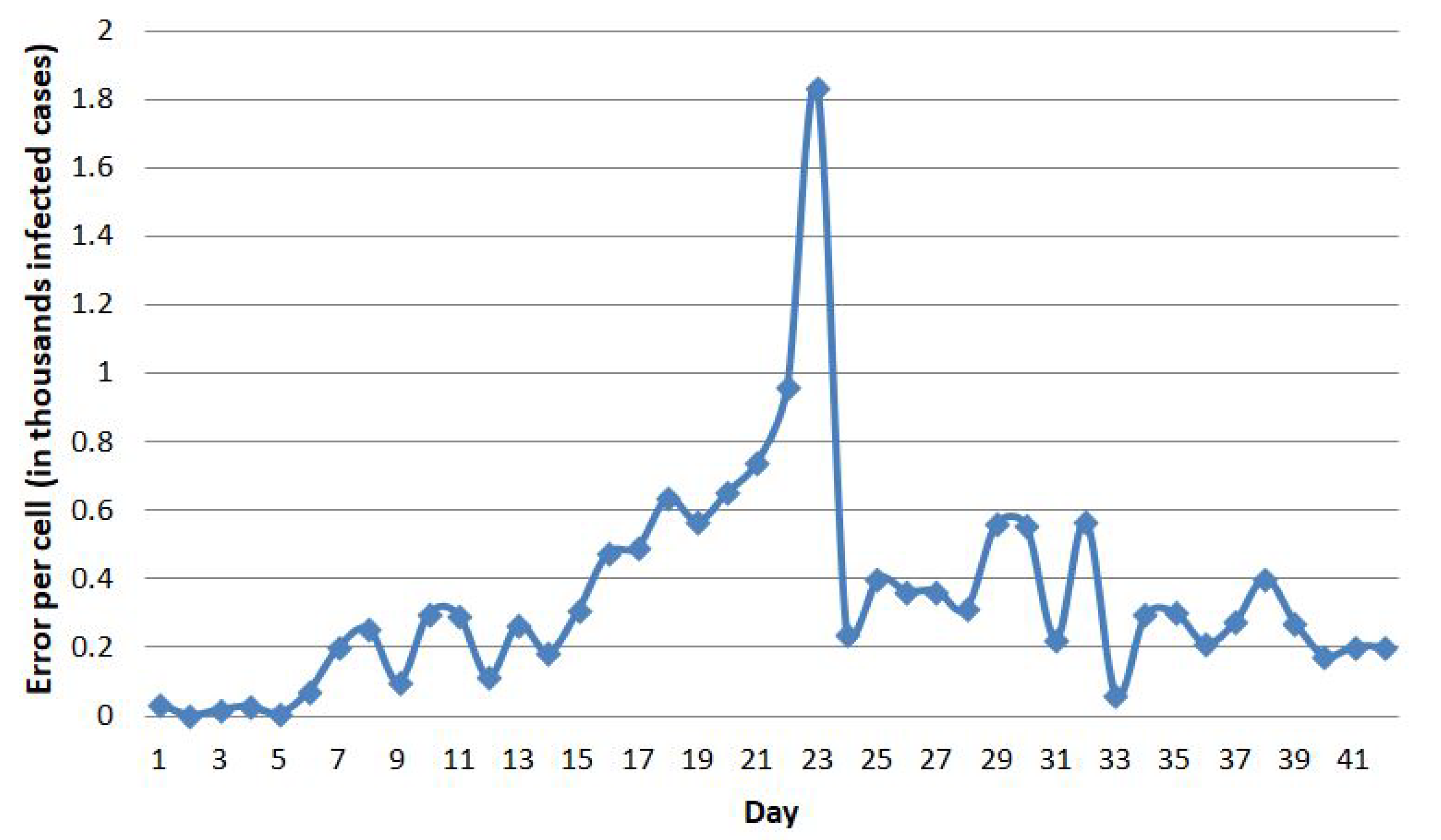
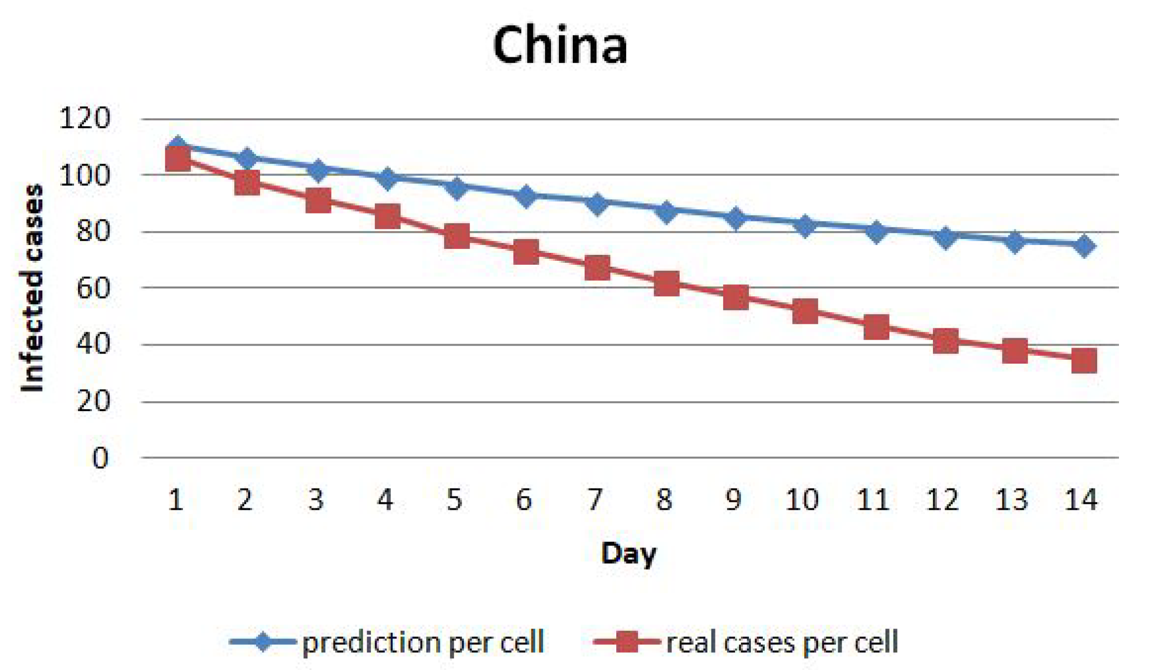
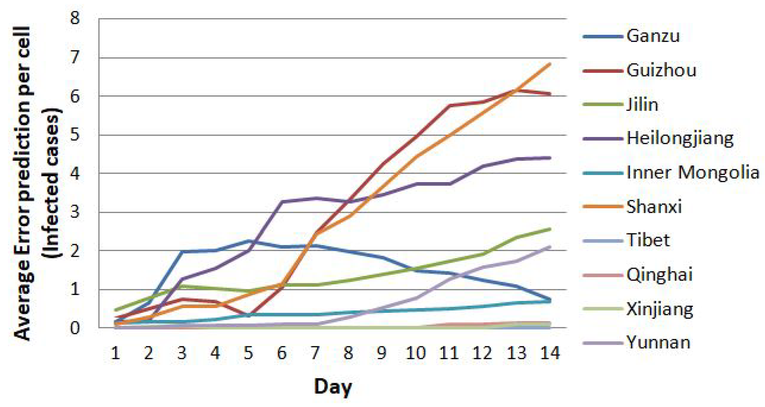
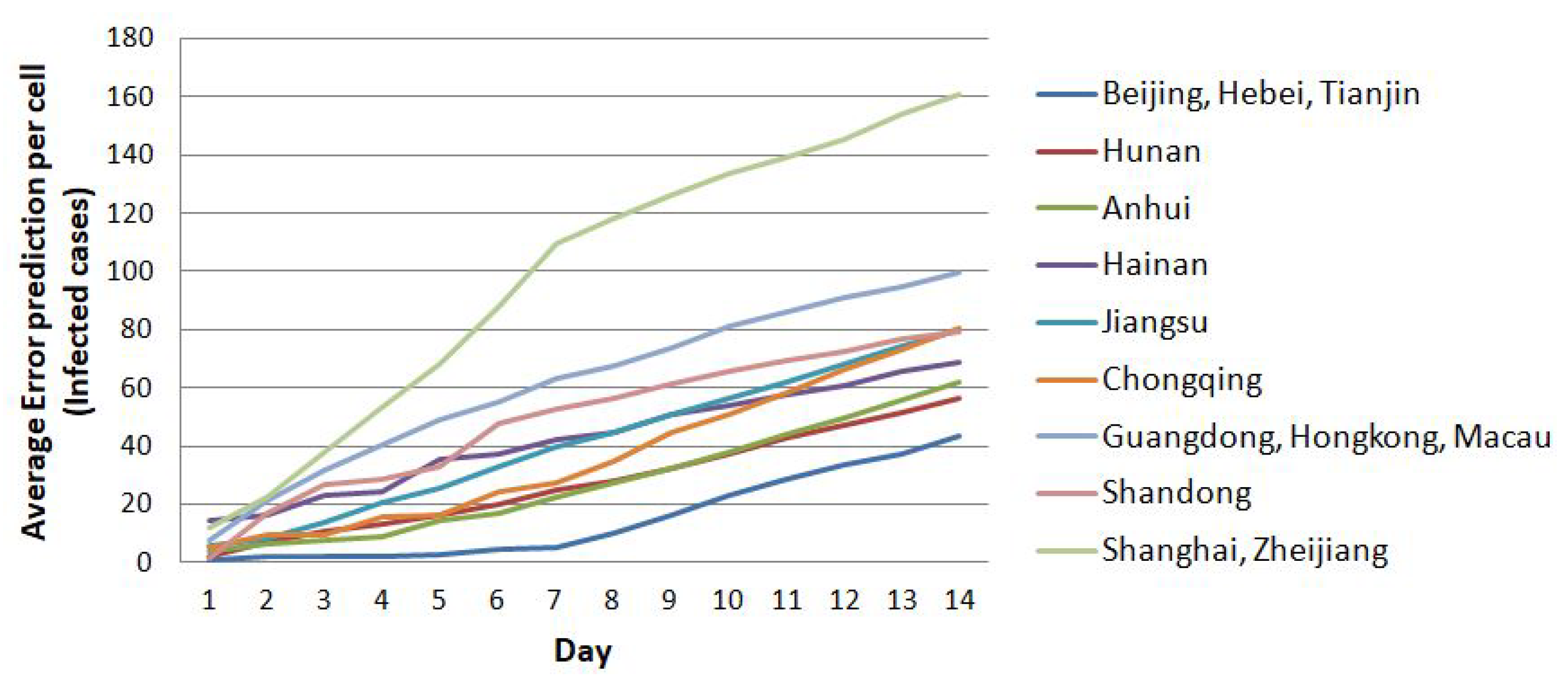
From the results (Figure 15, Figure 16 and Figure 17) in Section 4.2, we can see that the error for predictions up to day 14 is relatively small (ranging between 0 and 160), except for Hubei. This study compares the baseline model from Fong et al. [43] that used a Composite Monte-Carlo method simulation, enhanced by a deep learning network and fuzzy rule induction applying to limited data. The baseline model forecasts the overall trend and propagation of the infected cases during the early epidemic influenced by the temporal-spatial data of the nearby cities around China. The model uses the same number of future days to forecast, i.e., for the next 14 days, for China and obtains an RMSE of about 62,077.26. Meanwhile, in our study, the total RMSE in China was only 6631.42, about ten times smaller (

Table 2. RMSE for 7- and 14-day predictions.

ID	Region	RMSE for 7 Days	RMSE for 14 Days
1	Anhui	12.99	33.65
2	Beijing, Heibei, Tianjin	3.04	21.04
3	Chongqing	17.25	44.35
4	Fujian	14.55	20.22
5	Gansu	1.79	1.63
6	Guangdong, Hongkong, Macau	42.32	67.43
7	Guangxi	2.82	6.93
8	Guizhou	1.12	3.82
9	Hainan	29.26	45.91
10	Heilongjiang	2.07	3.12
11	Henan	1.49	10.78
12	Hubei	596.60	976.42
13	Hunan	15.23	32.45
14	Inner Mongolia	0.26	0.42
15	Jiangsu	24.14	48.02
16	Jiangxi	6.24	7.10
17	Jilin	0.96	1.49
18	Liaoning	1.61	5.82
19	Ningxia	2.10	18.33
20	Qinghai	0	0.07
21	Shaanxi	1.86	12.06
22	Shandong	33.69	54.43
23	Shanghai, Zhejiang	64.62	109.25
24	Shanxi	1.12	3.69
25	Sichuan	3.41	7.25
26	Tibet	0	0
27	Xinjiang	0.03	0.04
28	Yunnan	0.08	0.94
	All of China	3834.17	6631.42
	Baseline model [43] (the baseline only provides a single average RMSE in China influenced by the temporal-spatial data of nearby cities around Wuhan).	N/A	62,077.26

).

From the error analysis using RMSE (Equation (22)) as shown in Table 2, the data that caused the unexpected prediction results were outliers, such as the case in Hubei. The outlier was interesting since there was a crowded traditional market full of visitors in the city of Wuhan. We can propose the outlier as a separate study.

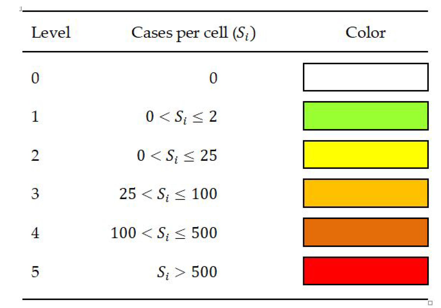
The results of visualizing the spreading pattern of COVID-19 for eight weeks, in Figure 8, show that Hubei is constantly in the red area, which implies that this area remains the center of the disease spread. However, it also causes a high average of the training error, which means Hubei is outlier data. However, as a method with spatial characteristics, CA turned out to be pretty reasonable to model the spread of disease. It demonstrated that the CA model could enhance the accuracy of the prediction model by increasing the amount of training data or adding other related factors that influenced the spreading of disease.

Compared to previous studies in epidemiology, mainly related to COVID-19 at the beginning of the outbreak, our proposed model can show the visualization of the result on the level of vulnerability. Thus, the model can directly observe the position of clusters of regions. Until the end of 2020, the previous related study still used a mathematical model and statistical data processing for calculating the parameters of the epidemiological model of COVID-19 in Wuhan. It uses a graphical representation (chart) for showing the tendency of spreading without including spatial information [9,51]. Thus, the ability to represent the COVID-19 outbreak with spatial information can significantly contribute to the COVID-19 spreading model. We expect that the visualization based on spatial information could help the decision-maker determine a more precise policy.

The advantage of using CA is that the prediction results are more precise than standard forecasting methods for the whole data set. One of the reasons is that we can divide the COVID-19 data into small regions. Thus, we can analyze separately by considering the influence and behavior of its neighborhood, whereas standard forecasting methods override the influence of a neighborhood. However, the drawback of the model is the difficulty in defining cellular space. The configuration of cellular space and the definition of a neighborhood is not generic. Thus, we should redefine them to adjust the model if the characteristics of the problem and data set change. In addition, finding the optimal parameters is time-consuming and involves an array of variables that are sometimes more than two dimensions.

6. Conclusions

We succeeded in representing the influence of neighboring regions in COVID-19 epidemiological modeling, which we have proposed as the N-CCA model for our contribution. The N-CCA model has succeeded in modeling the influence of neighborhood interactions on the spread of COVID-19 in a region. In this study, we propose the N-CCA model, a non-uniform continuous CA-based approach combined with multiple regression to determine the coefficients representing the magnitude of the interaction influence.

We apply the N-CCA model to predict the spread of COVID-19 cases in China. We developed a prediction model using 42 days of cases as a training data set and using the next 14 days as a validation data set to evaluate the model’s prediction results. We used RMSE to calculate the prediction error on the average number of cases for each cell in a region. We obtain the RMSE values in the length range 0–42.32 and 0–67.43 per cell for 7 and 14 days of prediction except for Hubei. Meanwhile, the RMSE for all of China is about 6631.42. Thus, our overall model is better than the baseline.

The CA method has an opportunity to improve the predictive model of disease spread. We can improve the model by including other parameters, e.g., vaccination, comorbidity, and isolation factors. Moreover, we can also change the definition of cellular space, such as changing the number of cells and changing the membership definition of each cell. We can conduct another improvement by using the Moore neighborhood as a neighborhood frame model. Lastly, we can consider the population density when calculating the case spreading.

One of the challenges of using the CA approach in modeling disease spread is to define different cellular spaces for other geographic and demographic conditions. In addition, in this study, the number of regression problems that must be solved is 258, which is as many as the number of cells defined. If there are more cells and neighbors and the model has a more complex factor involvement, we can use machine learning or deep learning to solve the regression problems to obtain a predictive model with the CA approach.

The current study uses time-series data that are limited to 42 days. In future work, there are several things we can try to improve the accuracy, including adding time series data and an explicit movement factor, among others. For building a predictive model, adding more data can solve using machine learning for time series data. In addition, the consequence of adding an explicit movement factor needs modification of the design of the predictive model.