
A Novel Approach to Learning Models on EEG Data Using Graph Theory Features—A Comparative Study


Abstract
:1. Introduction
2. Materials and Methods
2.1. Datasets
2.2. Computation of Correlation Matrix and Time Resolved Correlation Matrix Using Brainstorm Toolbox
- The EEG sensors data is used from each of the datasets.
- Trail based data is drawn on.
- Full networks are calculated.
- In terms of temporal resolution, both static and dynamic are studied.
- The output data has a 4-D structure: Channels X Channels X Frequency Bands X Time.
2.2.1. Correlation Matrix Computation
- The Input option has three input fields, namely:
- (a)
- Time window.
- (b)
- Sensors types or names.
- (c)
- Checkbox to include bad channels.
- The process option has a checkbox to allow for computing the scalar product instead of correlation.
- Finally, output options, which has two checkboxes: (1) for saving individuals’ results (one file per input file) and (2) for saving the average connectivity matrix (one file).
2.2.2. Time Resolved Matrix Computation
- Input option has three input fields:
- (a)
- Time window.
- (b)
- Sensor types or names and a checkbox to include bad channels.
- Process option has:
- Estimation window length (350 ms).
- Sliding window overlap (50%).
- Estimator options: computing the scalar product instead of correlation.
- Output configuration (enables addition of comment tag).
2.3. Methods
Data Processing
2.4. Learning Models
2.4.1. The Logistic Regression Model (LR)
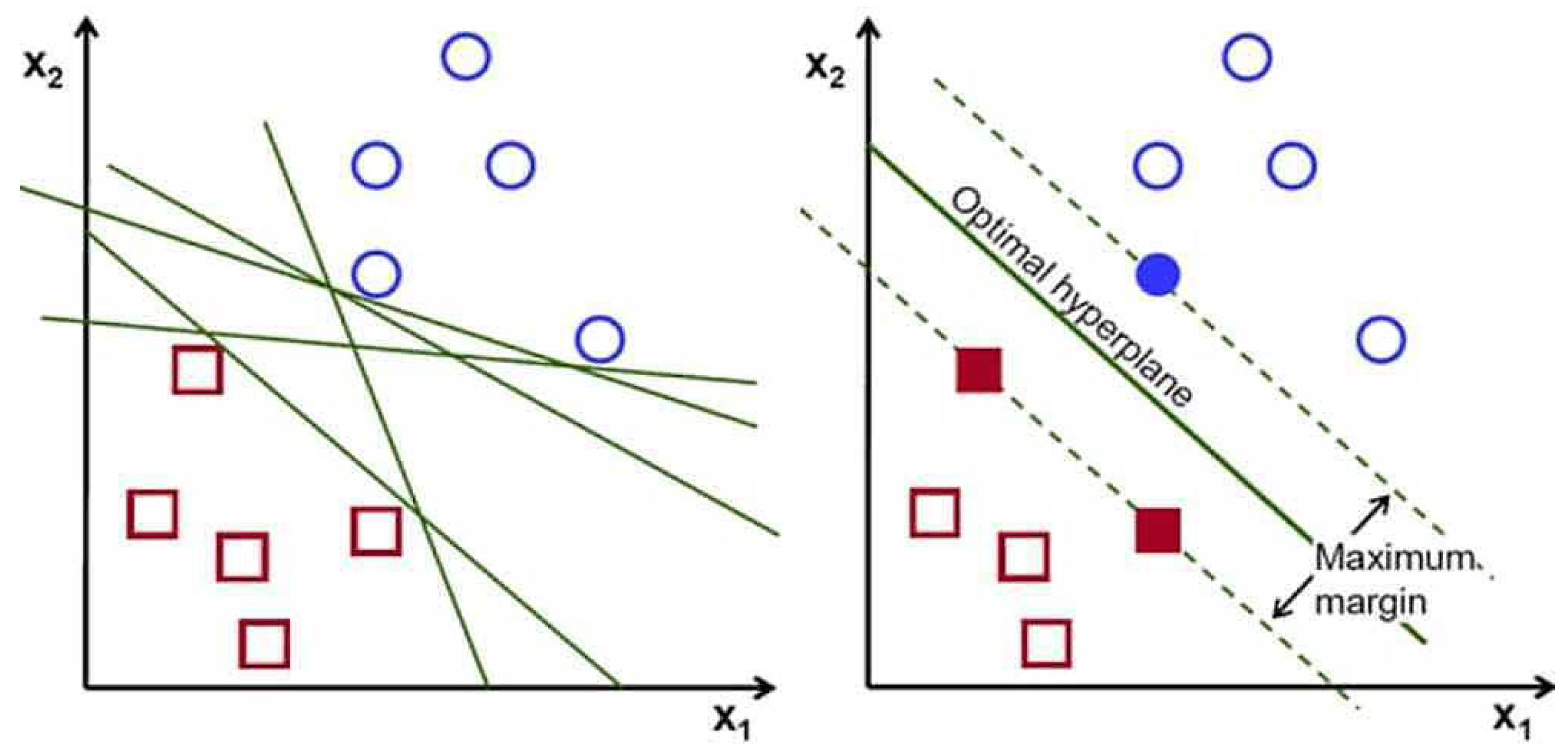
2.4.2. Support Vector Machine (SVM)
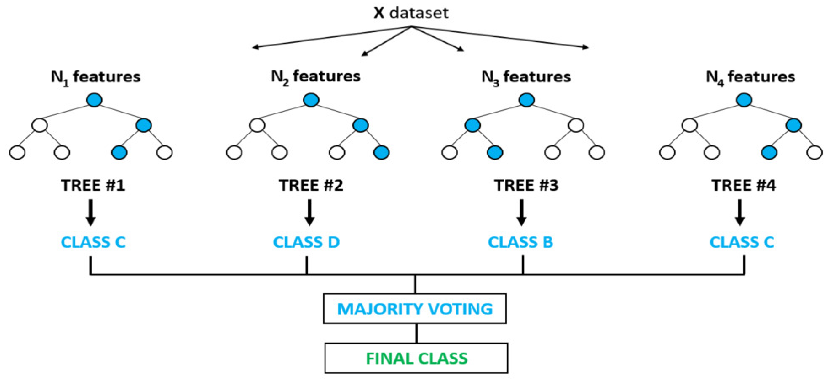
2.4.3. Random Forest (RF)
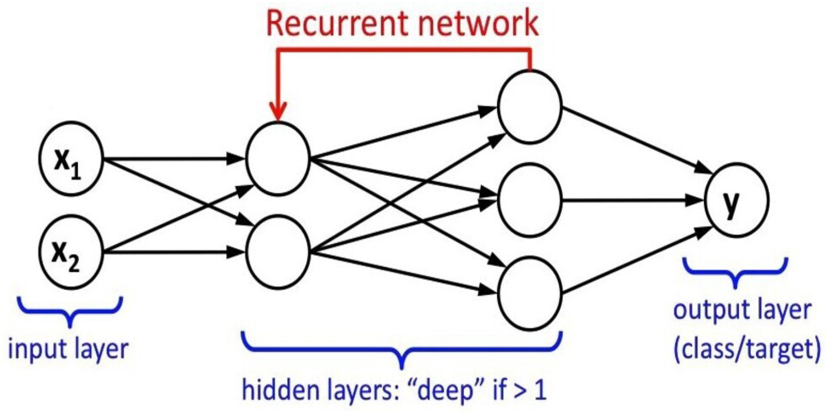
2.4.4. Recurrent Neural Network (RNN)
3. Results
4. Discussion
4.1. Limitations
5. Conclusions
Author Contributions
Funding
Institutional Review Board Statement
Informed Consent Statement
Data Availability Statement
- EEG: Visual Working Memory + Carbergoline Challenge DatasetDOI:10.18112/openneuro.ds003519.v1.1.0,
- EEG: Probabilistic selection task and Depression DatasetDOI:10.18112/openneuro.ds003474.v1.1.0,
- VerbalWorkingMemory DatasetDOI:10.18112/openneuro.ds003655.v1.0.0.
- DASS 21 Questionnaire EEG recordings-https://tinyurl.com/cvd729p8 and
- Working Memory EEG recordings-https://tinyurl.com/2z6ms7p6
Conflicts of Interest
Appendix A
Reproduction of the Research Shown
- in-house EEG datasets please follow the steps provided below
- import the files to EEGLab on MATLAB
- filter the files using the MARA Toolbox using band-pass filter 0.1–70 Hz and 50 Hz notch filter
- please select automatic ICA rejection
- export the files as .set format
- import the files (create a study for each dataset) on to brainstorm toolbox on MATLAB.
- use the connectivity editor for computing Correlation Matrix
- For the OpenNEURO datasets
- import the files(create a suitable study protocol for each dataset) on to brainstorm
- use the connectivity editor for computing Correlation Matrix
- In case the files on OpenNEURO are RAW files, follow the steps provided on the readme file for preprocessing of the EEG recordings.

| Condition | Logistic Regression (% Accuracy) | Random Forest (% Accuracy) | SVM (% Accuracy) | RNN (% Accuracy) |
|---|---|---|---|---|
| Placebo | 73.60 | 80.40 | 73.50 | 90.20 |
| Drug | 71.80 | 81.60 | 76.80 | 92.80 |
| 5 | 6 | 7 | |
|---|---|---|---|
| Manipulation | Logistic regression–66.66% Random forest–65.50% SVM–60.15% RNN–75.86% | Logistic regression–59.40% Random forest–69.40% SVM–59.80% RNN–70.40% | Logistic regression–61.10% Random forest–76.70% SVM–54.70.10% RNN–71.50% |
| Retention | Logistic regression–68.70% Random forest–70.60% SVM–55.60% RNN–74.80% | Logistic regression–66.40% Random forest–65.80% SVM–50.20% RNN–70.60% | Logistic regression–63.40% Random forest–68.30% SVM–53.30% RNN–79.60% |
| Logistic Regression (% Accuracy) | Random Forest (% Accuracy) | SVM (% Accuracy) | RNN (% Accuracy) | |
|---|---|---|---|---|
| Participant 01 | 12.5 | 37.5 | 28.60 | 12.5 |
| Participant 02 | 25 | 28.30 | 28.60 | 28.60 |
| Participant 03 | 14.30 | 37.5 | 14.30 | 14.30 |
| Participant 04 | 50 | 12.5 | 25 | 25 |
| Participant 05 | 25 | 25 | 25 | 28.60 |
| Participant 06 | 25 | 12.5 | 12.5 | 14.30 |
| Participant 07 | 14.30 | 42.90 | 12.5 | 50 |
| Participant 08 | 12.5 | 25 | 12.5 | 12.5 |
| Participant 09 | 50 | 28.60 | 22.22 | 25 |
| Participant 10 | 75 | 50 | 14.60 | 14.60 |
| Participant 11 | 12.5 | 12.5 | 28.60 | 22.22 |
| Participant 12 | 37.5 | 50 | 11.11 | 12.5 |
| Participant 13 | 28.60 | 14.30 | 25 | 28.60 |
| Participant 14 | 12.5 | 12.5 | 37.5 | 14.30 |
| Participant 15 | 25 | 25 | 37.5 | 25 |
| Participant 16 | 25 | 12.5 | 12.5 | 12.5 |
| Participant 17 | 28.60 | 25 | 50 | 33.33 |
| Participant 18 | 12.5 | 37.5 | 25 | 14.60 |
| Participant 19 | 50 | 12.5 | 37.5 | 25 |
| Participant 20 | 14.30 | 14.30 | 14.30 | 12.5 |
| Participant 21 | 25 | 37.5 | 14.30 | 12.5 |
| Participant 22 | 12.5 | 25 | 22.22 | 14.30 |
| Participant 23 | 14.30 | 25 | 28.60 | 25 |
| Participant 24 | 25 | 12.5 | 12.5 | 28.60 |
| Participant 25 | 50 | 28.60 | 12.5 | 12.5 |
References
- Soufineyestani, M.; Dowling, D.; Khan, A. Electroencephalography (EEG) technology applications and available devices. Appl. Sci. 2020, 10, 7453. [Google Scholar] [CrossRef]
- Li, G.; Lee, C.H.; Jung, J.J.; Youn, Y.C.; Camacho, D. Deep learning for EEG data analytics: A survey. In Concurrency Computation; John Wiley and Sons Ltd.: Hoboken, NJ, USA, 2019. [Google Scholar] [CrossRef]
- Vecchio, F.; Miraglia, F.; Maria Rossini, P. Connectome: Graph theory application in functional brain network architecture. Clin. Neurophysiol. Pract. 2017, 2, 206–213. [Google Scholar] [CrossRef] [PubMed]
- Wendling, F.; Ansari-Asl, K.; Bartolomei, F.; Senhadji, L. From EEG signals to brain connectivity: A model-based evaluation of interdependence measures. J. Neurosci. Methods 2009, 183, 9–18. [Google Scholar] [CrossRef] [PubMed] [Green Version]
- Bashiri, M.; Mumtaz, W.; Malik, A.S.; Waqar, K. EEG-based brain connectivity analysis of working memory and attention. In Proceedings of the ISSBES 2015-IEEE Student Symposium in Biomedical Engineering and Sciences: By the Student for the Student, Shah Alam, Malaysia, 4 November 2015; pp. 41–45. [Google Scholar] [CrossRef]
- Chang, S.; Dong, W.; Jun, H. Use of electroencephalogram and long short-term memory networks to recognize design preferences of users toward architectural design alternatives. J. Comput. Des. Eng. 2020, 7, 551–562. [Google Scholar] [CrossRef]
- Krumpe, T.; Scharinger, C.; Rosenstiel, W.; Gerjets, P.; Spüler, M. Unity and diversity in working memory load: Evidence for the separability of the executive functions updating and inhibition using machine learning. bioRxiv 2018. [Google Scholar] [CrossRef]
- Wu, C.T.; Dillon, D.; Hsu, H.C.; Huang, S.; Barrick, E.; Liu, Y.H. Depression Detection Using Relative EEG Power Induced by Emotionally Positive Images and a Conformal Kernel Support Vector Machine. Appl. Sci. 2018, 8, 1244. [Google Scholar] [CrossRef]
- Kumar, P.; Garg, S.; Garg, A. Assessment of Anxiety, Depression and Stress using Machine Learning Models. Procedia Comput. Sci. 2020, 171, 1989–1998. [Google Scholar] [CrossRef]
- Priya, A.; Garg, S.; Tigga, N.P. Predicting Anxiety, Depression and Stress in Modern Life using Machine Learning Algorithms. Procedia Comput. Sci. 2020, 167, 1258–1267. [Google Scholar] [CrossRef]
- Hosseinifard, B.; Moradi, M.H.; Rostami, R. Classifying depression patients and normal subjects using machine learning techniques and nonlinear features from EEG signal. Comput. Methods Programs Biomed. 2013, 109, 339–345. [Google Scholar] [CrossRef]
- Schirrmeister, R.; Gemein, L.; Eggensperger, K.; Hutter, F.; Ball, T. Deep learning with convolutional neural networks for decoding and visualization of eeg pathology. arXiv 2017, arXiv:1708.08012. [Google Scholar]
- Johannesen, J.K.; Bi, J.; Jiang, R.; Kenney, J.G.; Chen, C.M.A. Machine learning identification of EEG features predicting working memory performance in schizophrenia and healthy adults. Neuropsychiatr. Electrophysiol. 2016, 2, 1–21. [Google Scholar] [CrossRef] [Green Version]
- Antonijevic, M.; Zivkovic, M.; Arsic, S.; Jevremovic, A. Using AI-Based Classification Techniques to Process EEG Data Collected during the Visual Short-Term Memory Assessment. J. Sens. 2020, 2020, 8767865. [Google Scholar] [CrossRef]
- Amin, H.U.; Mumtaz, W.; Subhani, A.R.; Saad, M.N.M.; Malik, A.S. Classification of EEG signals based on pattern recognition approach. Front. Comput. Neurosci. 2017, 11, 103. [Google Scholar] [CrossRef] [Green Version]
- Ruiz-Gómez, S.J.; Hornero, R.; Poza, J.; Santamar’ia-Vázquez, E.; Rodr’iguez-González, V.; Maturana-Candelas, A.; Gómez, C. A new method to build multiplex networks using canonical correlation analysis for the characterization of the Alzheimer’s disease continuum. J. Neural Eng. 2021, 18, 26002. [Google Scholar] [CrossRef] [PubMed]
- Tanaka, H.; Miyakoshi, M. Cross-correlation task-related component analysis (xTRCA) for enhancing evoked and induced responses of event-related potentials. NeuroImage 2019, 197, 177–190. [Google Scholar] [CrossRef] [PubMed]
- Perinelli, A.; Chiari, D.E.; Ricci, L. Correlation in brain networks at different time scale resolution. Chaos 2018, 28, 063127. [Google Scholar] [CrossRef] [PubMed]
- Bastos, A.M.; Schoffelen, J.M. A tutorial review of functional connectivity analysis methods and their interpretational pitfalls. Front. Syst. Neurosci. 2016, 9, 175. [Google Scholar] [CrossRef] [Green Version]
- Delorme, A.; Makeig, S. EEGLAB: An open source toolbox for analysis of single-trial EEG dynamics including independent component analysis. J. Neurosci. Methods 2004, 134, 9–21. [Google Scholar] [CrossRef] [PubMed] [Green Version]
- Anthony, J.B.; Makeig, S.T.P.J.T.J.S. Independent Componenet Analysis of Electroencephalographic Data. Adv. Neural Inf. Process. Syst. 1996, 91, 145–151. [Google Scholar]
- Winkler, I.; Haufe, S.; Tangermann, M. Automatic Classification of Artifactual ICA-Components for Artifact Removal in EEG Signals. Behav. Brain Funct. 2011, 7, 30. [Google Scholar] [CrossRef] [PubMed] [Green Version]
- Julian, L.J. Measures of Anxiety. Arthritis Care 2011, 63, 1–11. [Google Scholar] [CrossRef] [PubMed] [Green Version]
- Cavanagh, J.F. EEG: Probabilistic Selection and Depression. 2021. Available online: https://openneuro.org/datasets/ds003474/versions/1.1.0 (accessed on 26 August 2021). [CrossRef]
- Nolan, H.; Whelan, R.; Reilly, R.B. FASTER: Fully Automated Statistical Thresholding for EEG artifact Rejection. J. Neurosci. Methods 2010, 192, 152–162. [Google Scholar] [CrossRef] [PubMed]
- Cavanagh, J.F.; Masters, S.E.; Bath, K.; Frank, M.J. Conflict acts as an implicit cost in reinforcement learning. Nat. Commun. 2014, 5, 5394. [Google Scholar] [CrossRef] [Green Version]
- Broadway, J.M.; Frank, M.J.; Cavanagh, J.F. Dopamine D2 agonist affects visuospatial working memory distractor interference depending on individual differences in baseline working memory span. Cogn. Affect. Behav. Neurosci. 2018, 18, 509–520. [Google Scholar] [CrossRef]
- Cavanagh, J.F.; Frank, M.J.; Broadway, J. EEG: Visual Working Memory + Cabergoline Challenge. OpenNeuro 2021. [Google Scholar] [CrossRef]
- Pavlov, Y.G. EEG: verbal working memory. OpenNeuro. 2021. [Google Scholar] [CrossRef]
- Palmer, J.; Kreutz-Delgado, K.; Makeig, S. AMICA: An Adaptive Mixture of Independent Component Analyzers with Shared Components; Technical Report; Swartz Center for Computational Neuroscience: San Diego, CA, USA, 2011; pp. 1–15. [Google Scholar]
- Pavlov, Y.G.; Kotchoubey, B.; Pavlov, Y.G. Temporally distinct oscillatory codes of retention and manipulation of verbal working memory Corresponding author. bioRxiv 2021. [Google Scholar] [CrossRef]
- Tadel, F.; Baillet, S.; Mosher, J.C.; Pantazis, D.; Leahy, R.M. Brainstorm: A User-Friendly Application for MEG/EEG Analysis. Comput. Intell. Neurosci. 2011, 2011, 879716. [Google Scholar] [CrossRef]
- Rubinov, M.; Sporns, O. Complex network measures of brain connectivity: Uses and interpretations. NeuroImage 2010, 52, 1059–1069. [Google Scholar] [CrossRef]
- Pedregosa, F.; Varoquaux, G.; Gramfort, A.; Michel, V.; Thirion, B.; Grisel, O.; Blondel, M.; Prettenhofer, P.; Weiss, R.; Dubourg, V.; et al. Scikit-learn: Machine Learning in Python. J. Mach. Learn. Res. 2011, 12, 2825–2830. [Google Scholar] [CrossRef]
- Gao, S.; Calhoun, V.D.; Sui, J. Machine learning in major depression: From classification to treatment outcome prediction. CNS Neurosci. Ther. 2018, 24, 1037–1052. [Google Scholar] [CrossRef] [Green Version]
- Dhanapal, R.; Bhanu, D. Electroencephalogram classification using various artificial neural networks. J. Crit. Rev. 2020, 7, 891–894. [Google Scholar] [CrossRef]
- Jiao, Z.; Gao, X.; Wang, Y.; Li, J.; Xu, H. Deep Convolutional Neural Networks for mental load classification based on EEG data. Pattern Recognit. 2018, 76, 582–595. [Google Scholar] [CrossRef]
- Kuanar, S.; Athitsos, V.; Pradhan, N.; Mishra, A.; Rao, K.R. Cognitive Analysis of Working Memory Load from Eeg, by a Deep Recurrent Neural Network. In Proceedings of the ICASSP, IEEE International Conference on Acoustics, Speech and Signal Processing-Proceedings, Calgary, AB, Canada, 15–20 April 2018; pp. 2576–2580. [Google Scholar] [CrossRef]
- Bilucaglia, M.; Duma, G.M.; Mento, G.; Semenzato, L.; Tressoldi, P. Applying machine learning EEG signal classification to emotion-related brain anticipatory activity. F1000Research 2020, 9, 173. [Google Scholar] [CrossRef] [Green Version]
- Craik, A.; He, Y.; Contreras-Vidal, J.L. Deep learning for electroencephalogram (EEG) classification tasks: A review. J. Neural Eng. 2019, 16, 031001. [Google Scholar] [CrossRef]
- Medvedev, A.V.; Agoureeva, G.I.; Murro, A.M. A Long Short-Term Memory neural network for the detection of epileptiform spikes and high frequency oscillations. Sci. Rep. 2019, 9, 19374. [Google Scholar] [CrossRef] [Green Version]
- Pavlov, Y.G.; Kotchoubey, B. The electrophysiological underpinnings of variation in verbal working memory capacity. Sci. Rep. 2020, 10, 16090. [Google Scholar] [CrossRef]
- Patel, M.J.; Khalaf, A.; Aizenstein, H.J. Studying depression using imaging and machine learning methods. Neuroimage Clin. 2016, 10, 115–123. [Google Scholar] [CrossRef] [PubMed] [Green Version]
- Pessoa, L. Understanding emotion with brain networks. Curr. Opin. Behav. Sci. 2018, 176, 19–25. [Google Scholar] [CrossRef] [PubMed]
- Cavanagh, J.F.; Bismark, A.W.; Frank, M.J.; Allen, J.J.B. Multiple Dissociations Between Comorbid Depression and Anxiety on Reward and Punishment Processing: Evidence From Computationally Informed EEG. Comput. Psychiatry 2019, 3, 1. [Google Scholar] [CrossRef] [PubMed]
- Zaharchuk, H.A.; Karuza, E.A. Multilayer networks: An untapped tool for understanding bilingual neurocognition. Brain Lang. 2021, 220, 104977. [Google Scholar] [CrossRef] [PubMed]
- Sharma, A.; Verbeke, W.J.M.I. Improving Diagnosis of Depression With XGBOOST Machine Learning Model and a Large Biomarkers Dutch Dataset (n = 11,081). Front. Big Data 2020, 3, 15. [Google Scholar] [CrossRef] [PubMed]


| Sl. No. | Name of the Dataset | EEG Recording System | Acquisition Parameters |
|---|---|---|---|
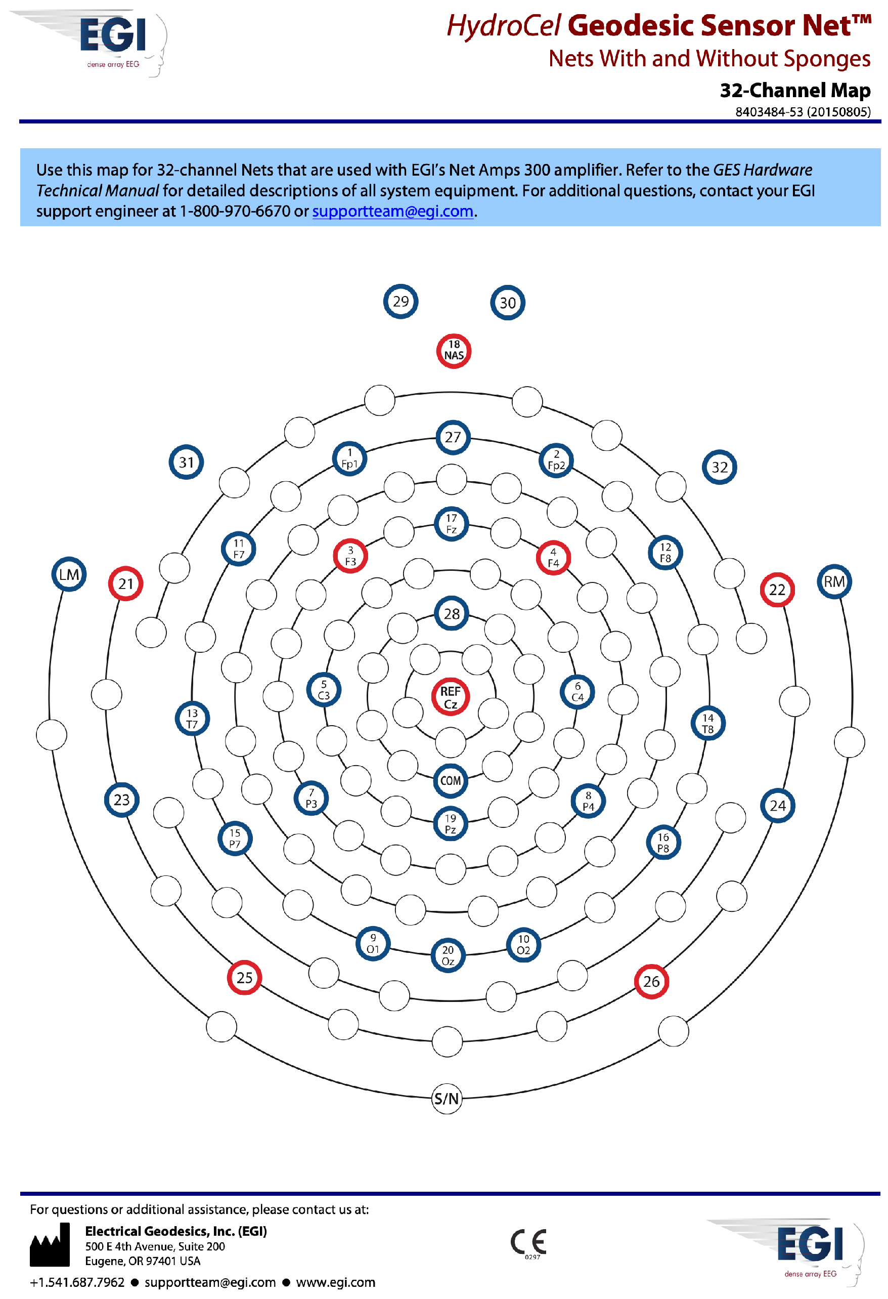
| 1 | Visual Working Memory (n = 25) | 32 Channel EGI geodesic | impedance < 50 k, 1000 Hz sampling rate, band-pass filter 0.1–70 Hz, 50 Hz notch filter |
| 2 | Visual Working Memory (n = 27) | 64-channel Brain Vision system | 500 Hz sampling rate, Band-pass filter 0.1–100 Hz |
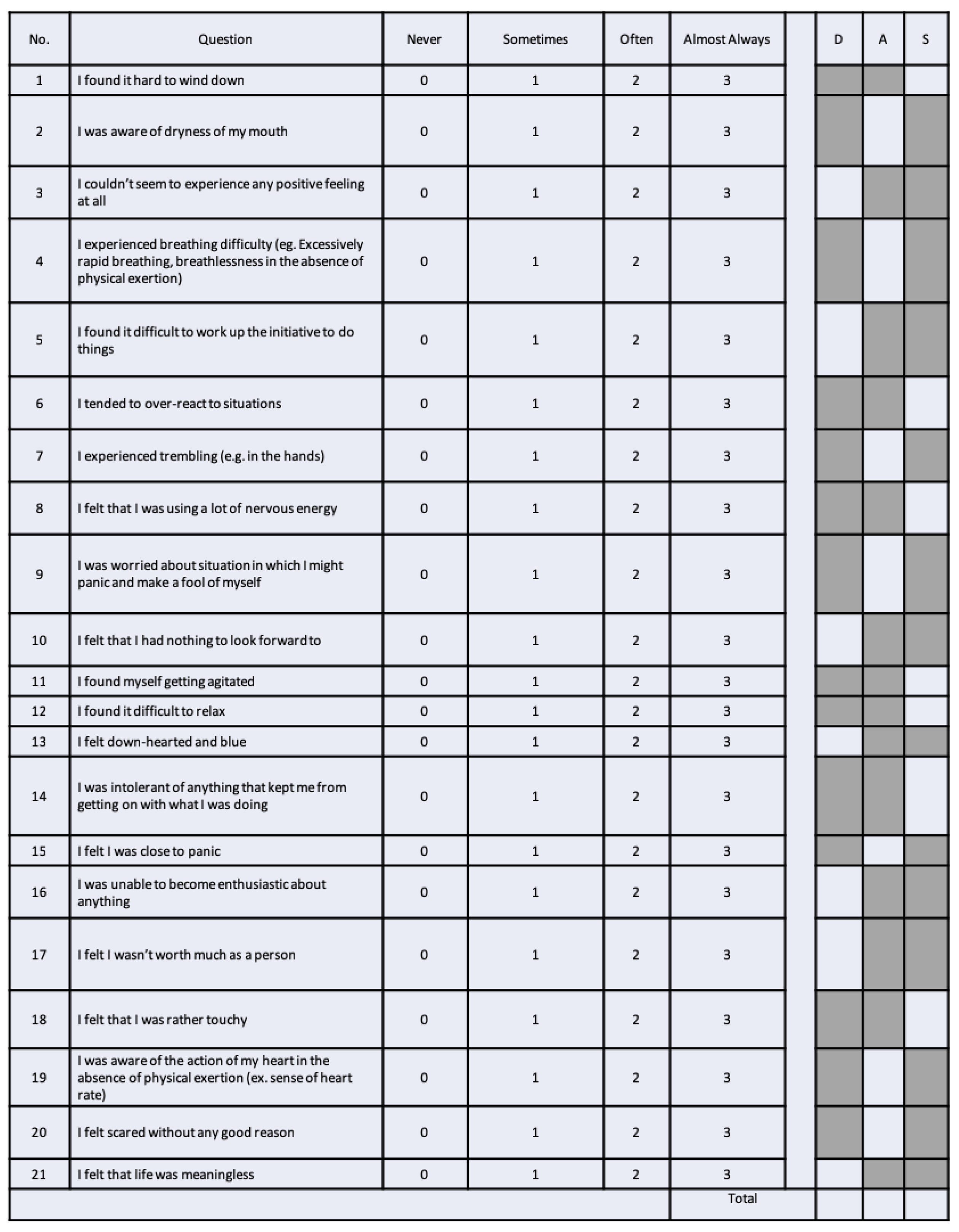
| 3 | DASS 21 Questionnaire (n = 29) | 32 Channel EGI geodesic | impedance < 50 k, 250 Hz sampling rate, band-pass filter 0.1–70 Hz, 50 Hz notch filter |
| 4 | Probabilistic Selection and Depression (n = 122) | 64 Ag/AgCl electrodes Synamps2 system | impedance < 10 k, 500 Hz sampling rate, band-pass filter 0.5–100 Hz |
| 5 | Verbal Working Memory (n = 156) | 19 electrodes 10–20 system Mitsar-EEG-202 amplifier | 500 Hz sampling rate, band-pass filter 1–150 Hz 50 Hz notch filter |
| Emotional State/ Learning Model Accuracy | Logistic Regression | Random Forest | SVM | RNN |
|---|---|---|---|---|
| Depression | 71.33% | 73.46% | 61.78% | 88.64 % |
| Anxiety | 64.56% | 78.66% | 65.27% | 80.75% |
| Emotional State/ (% Accuracy of Model) | Logistic Regression | Random Forest | SVM | RNN |
|---|---|---|---|---|
| Depression | 35.06% | 28.60% | 27.60% | 34.75% |
| Anxiety | 28.40% | 34.45% | 30.85% | 38.85% |
| Stress | 31.10% | 33.20% | 31.70% | 36.40% |
Publisher’s Note: MDPI stays neutral with regard to jurisdictional claims in published maps and institutional affiliations. |
© 2021 by the authors. Licensee MDPI, Basel, Switzerland. This article is an open access article distributed under the terms and conditions of the Creative Commons Attribution (CC BY) license (https://creativecommons.org/licenses/by/4.0/).
Share and Cite
Prakash, B.; Baboo, G.K.; Baths, V. A Novel Approach to Learning Models on EEG Data Using Graph Theory Features—A Comparative Study. Big Data Cogn. Comput. 2021, 5, 39. https://doi.org/10.3390/bdcc5030039
Prakash B, Baboo GK, Baths V. A Novel Approach to Learning Models on EEG Data Using Graph Theory Features—A Comparative Study. Big Data and Cognitive Computing. 2021; 5(3):39. https://doi.org/10.3390/bdcc5030039
Chicago/Turabian StylePrakash, Bhargav, Gautam Kumar Baboo, and Veeky Baths. 2021. "A Novel Approach to Learning Models on EEG Data Using Graph Theory Features—A Comparative Study" Big Data and Cognitive Computing 5, no. 3: 39. https://doi.org/10.3390/bdcc5030039
APA StylePrakash, B., Baboo, G. K., & Baths, V. (2021). A Novel Approach to Learning Models on EEG Data Using Graph Theory Features—A Comparative Study. Big Data and Cognitive Computing, 5(3), 39. https://doi.org/10.3390/bdcc5030039