This paper aims to identify modifications on the tweet text during preprocessing so that the resulting sentiment scores best correlated with Bitcoin’s closing prices. We created different ways of preprocessing text for VADER scoring and tested them on truncated and full-length tweets.
4.1. Data Collection
We gathered tweets for sentiment analysis by developing a custom tweet scraper using Twitter API. We chose to collect data for three main reasons manually. All existing online free datasets did not include the COVID-19 pandemic period. All web scrapers were avoided because they might bypass the restrictions of the Twitter API. These restrictions were meant to protect Twitter users. We followed twitters rules [
27,
28], and we coded our tweet scraper in Python using the Tweepy library to access the Twitter API [
29]. In our experiments, the collection method obtained a representative set of BTC tweets during the COVID-19 period. The tweet selection involved filtering tweets by a manually chosen set of keywords. Tweets that contained any keywords related to bitcoin (“bitcoin”, “bitcoins”, “Bitcoin”, “Bitcoins”, “BTC”, “XBT”, and “satoshi”) or any hashtags of Bitcoin’s ticker symbols (“#XBT”, “
$XBT”, “#BTC”, and “
$BTC”) were collected. Raw tweet text and their timestamps were stored. Timestamps were provided at a temporal resolution to the nearest second. As Twitter truncates tweets over 140 characters, the full-length version of those tweets was also collected [
30,
31,
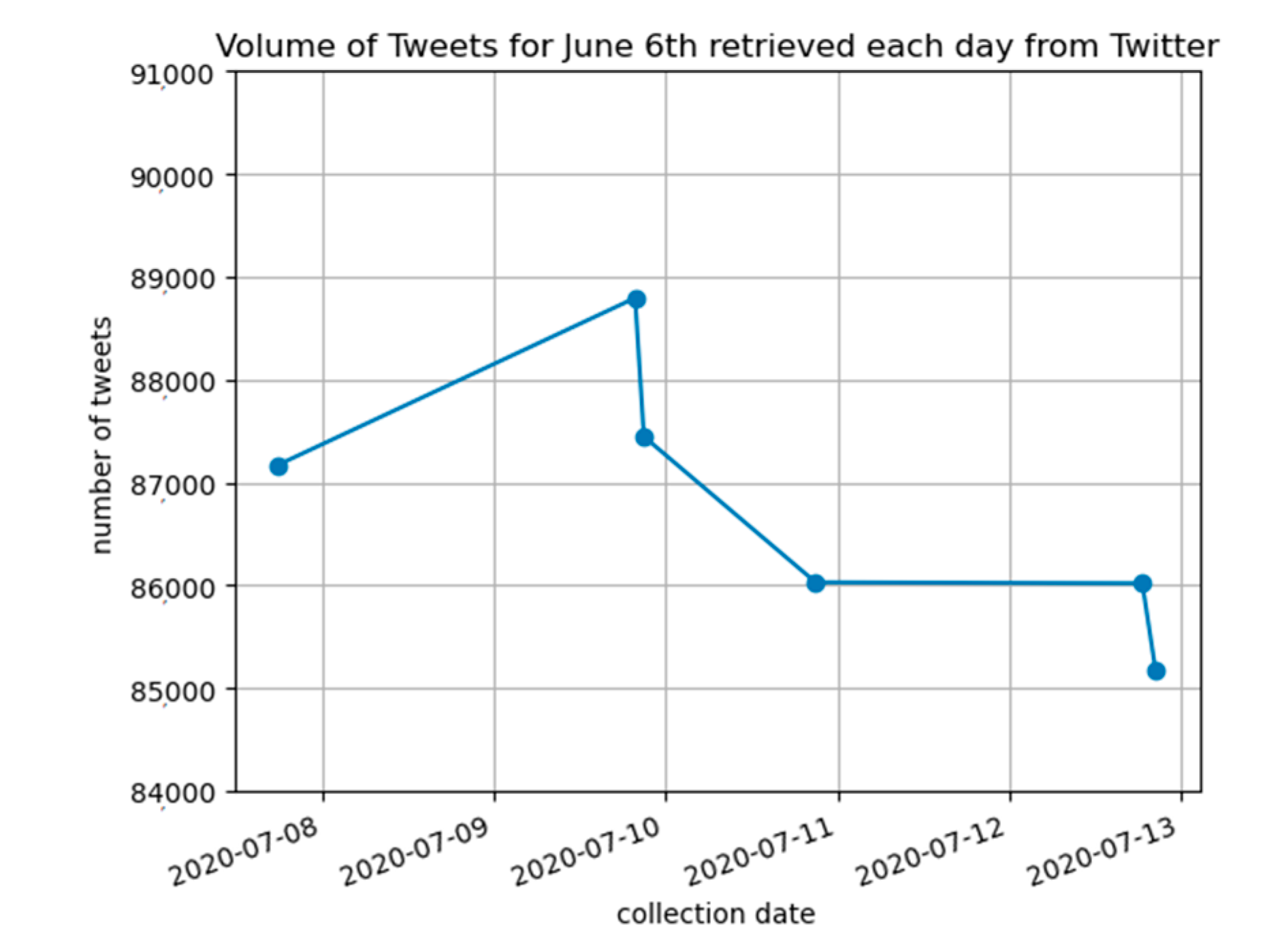
32]. A total of 4,169,709 tweets were collected from 8:47 AM, 22 May to 11:59 PM, 10 July. The volume of tweets collected for each date was observed to vary based on how old the requested data are, as shown in
Figure 1. Bitcoin prices are obtained for free from the CryptoCompare API [
32]. They provide open historical data of opening, high, low, and closing prices and volume (OHLCV) information at a temporal resolution of every minute [
33]. Minutely, Bitcoin data were obtained over hourly data to provide enough data points to analyze. About 71,472 min of data points was collected from 22 May to 10 July, while collecting hourly prices would have provided nearly 1191 data points. Timestamps of Bitcoin prices and OHLCV data were then stored. The recorded OHLCV data from (Cryptocompare.com) seemed to fluctuate when prices were still recent. Data were provided up to 33 h into the past (based on our tests). A bi-daily collection routine was used to replace any recent prices (near the start of the collection period) that matched timestamps with any older prices from the next collection period.
4.2. Data Preprocessing
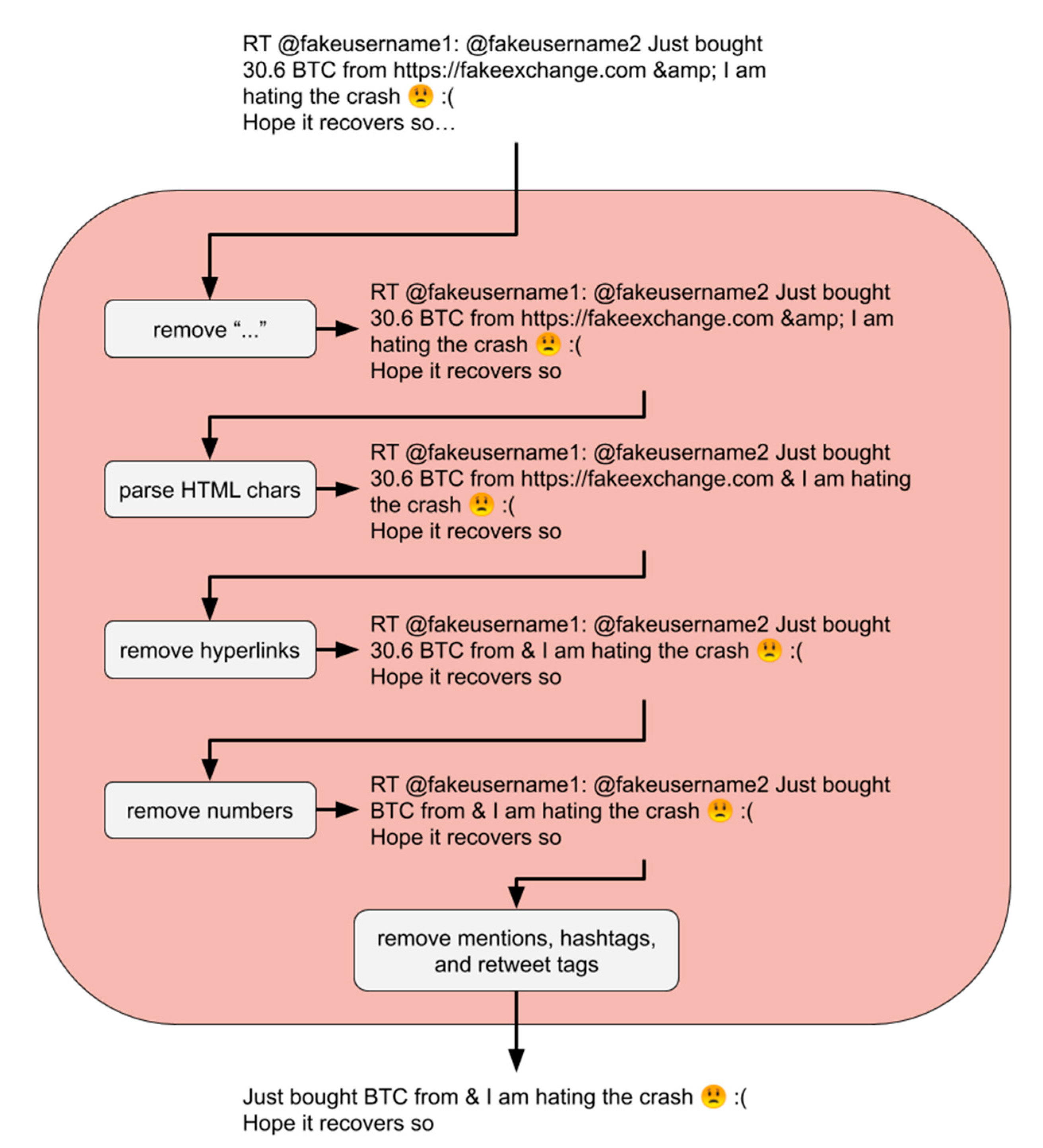
Preprocessing was performed on the text from each tweet converted into an average polarity score and tweet polarity volume per minute. This involves combining three main text cleaning functions labeled “cleaned,” “split,”, and “no sw”. Respectively, they managed the removal of tweet-specific syntax, splitting text into sentences, and removing stopwords. The “cleaned” and “split” functions were tested in different orders, with and without the presence of the “no sw” function at the end. All three preprocessing functions affected the VADER sentiment analysis of text in different ways. Each had the potential to significantly help VADER capture a different aspect of sentiment from the text. The “cleaned” function removed unwanted characters and words used specifically on Twitter’s platform, such as hyperlinks, numbers, and tweet specific syntax, using regular expressions. The removal was applied to preserve emojis and possible emoticon characters for use in the VADER sentiment analyzer. Before removing any alphanumeric chars, the ellipsis mark “…” was removed from the end of tweet text truncated to fit within 140 characters. Additionally, HTML entities such as “&” were converted to UTF-8 equivalent characters, such as “&”. Then hyperlinks starting with the characters “http” or “www.” were removed. Numbers, along with any symbols, punctuation, or units next to them, were removed. Finally, the tweet-specific syntax was removed. This syntax included mentions of usernames of the form “@username,” hashtags of the form “#hashtag” and the start of retweets of the form “RT @username.” Once the cleaning phase was completed as shown in
Figure 2, each tweet was represented by words, whitespace, emojis, and other non-alphanumeric characters. Due to the difficulty of creating a regular expression to recognize all emoticons in VADER’s lexicon [
34], these characters were left unchanged. Therefore, the “cleaned” text attempted to leave everything that VADER could use in sentiment analysis unchanged.
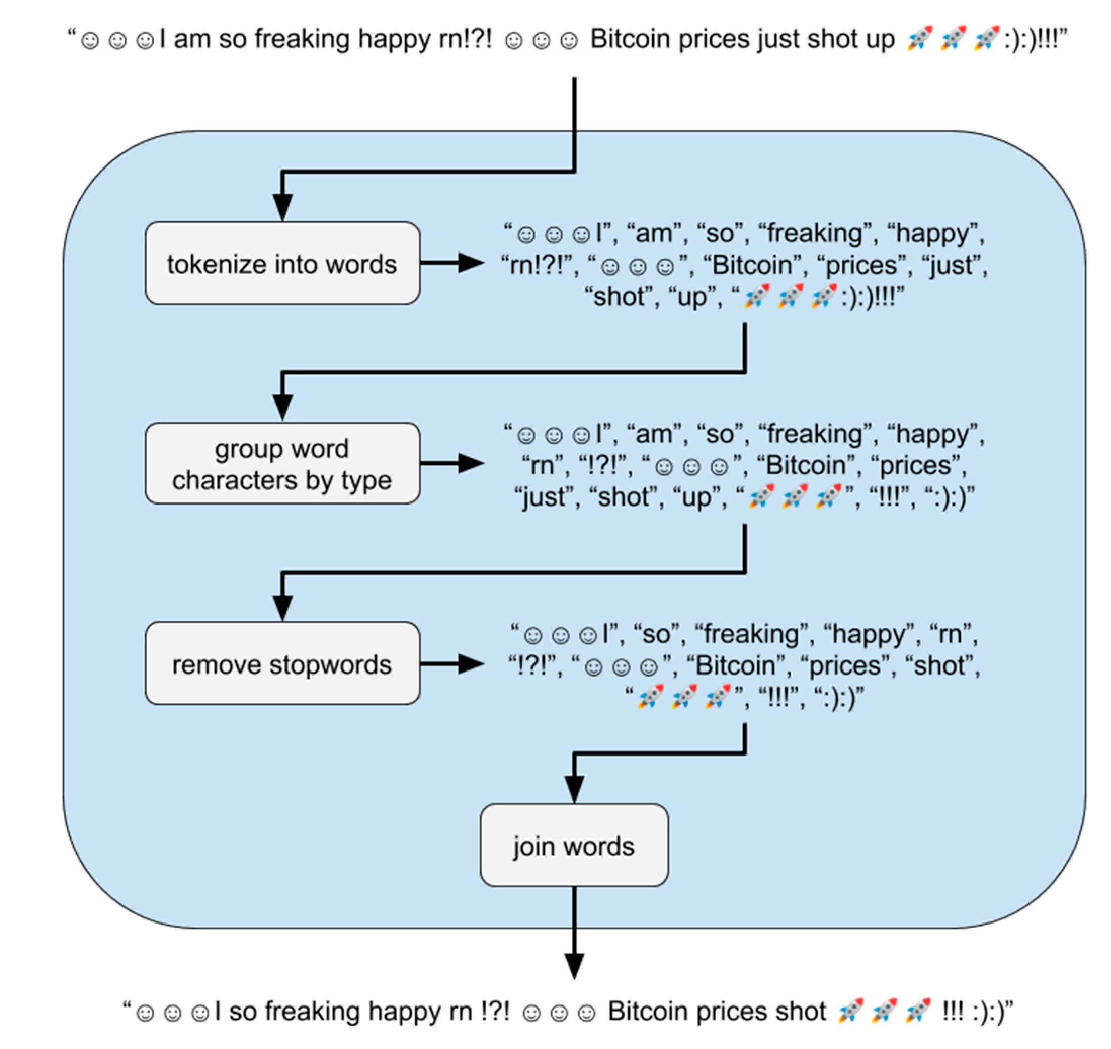
The “no sw” function in
Figure 3 tokenizes text into words and removes any stopwords that VADER’s dictionary does not use. Removing stop words from text requires a tokenized text into a list of words. The tokenization of text into words involves separating continuous blocks of alphabetical characters from the rest of the text. Blocks of continuous whitespace mark our word boundaries, split by Python’s split () function [
35]. Removing all non-alphabetical characters would solve this; however, this would remove some punctuation, all emojis, and all emoticons that VADER could recognize for sentiment analysis [
36]. VADER allows exclamation marks ”!” and question marks ”?”, which affect the sentiment score [
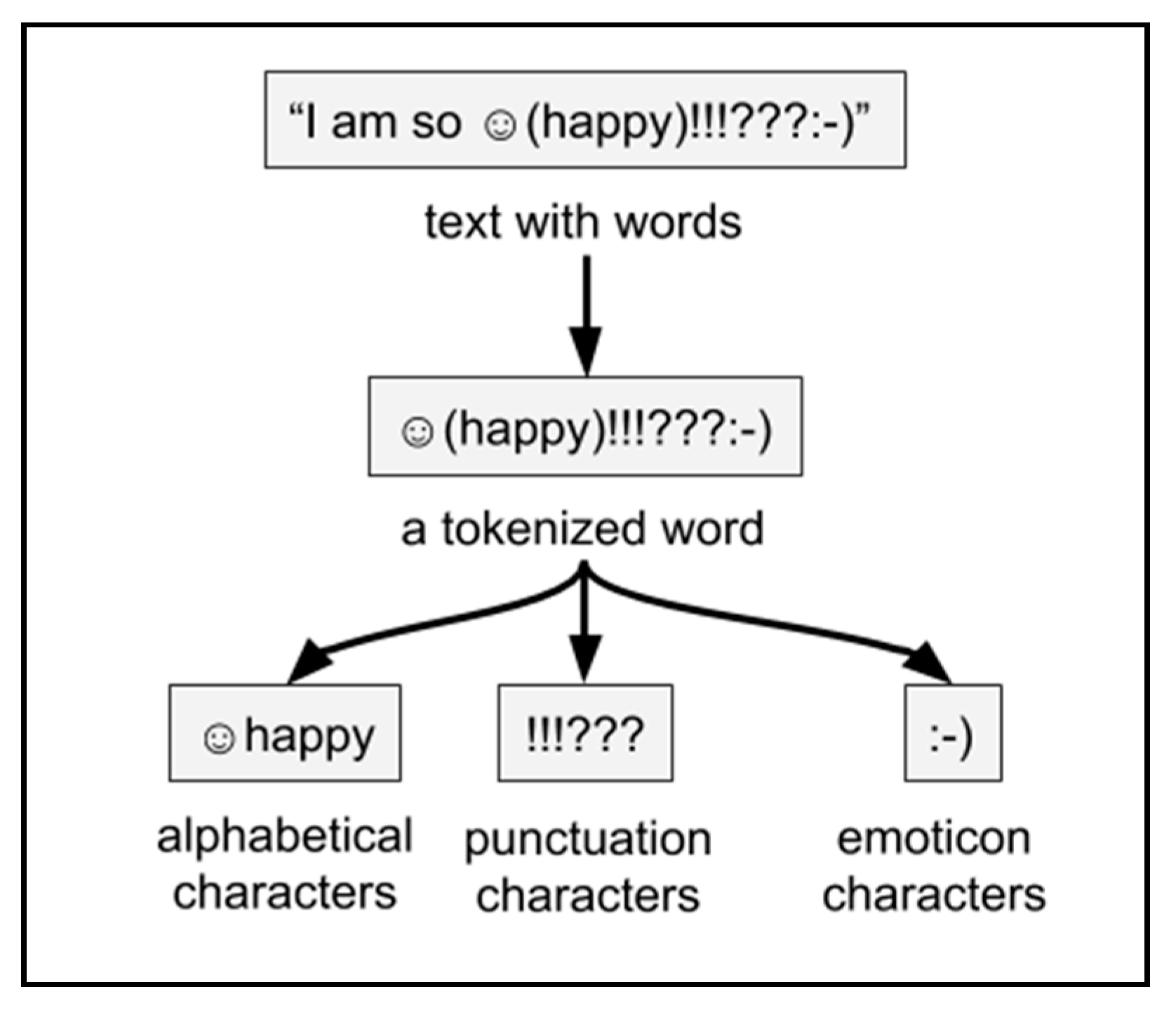
36]. Our tokenization algorithm, as shown in
Figure 4, groups characters from every tokenized word into “alphabetical”, “punctuation”, or “emoticon” blocks of characters. Ideally, these three blocks of characters would allow VADER to join each of them to preserve most of the text VADER can recognize. To distinguish punctuation from emoticons, any characters in the set
$=@&_*#>:`\</{})]|%;~-,([+^” are only part of an emoticon if they occur next to another character in the same set.
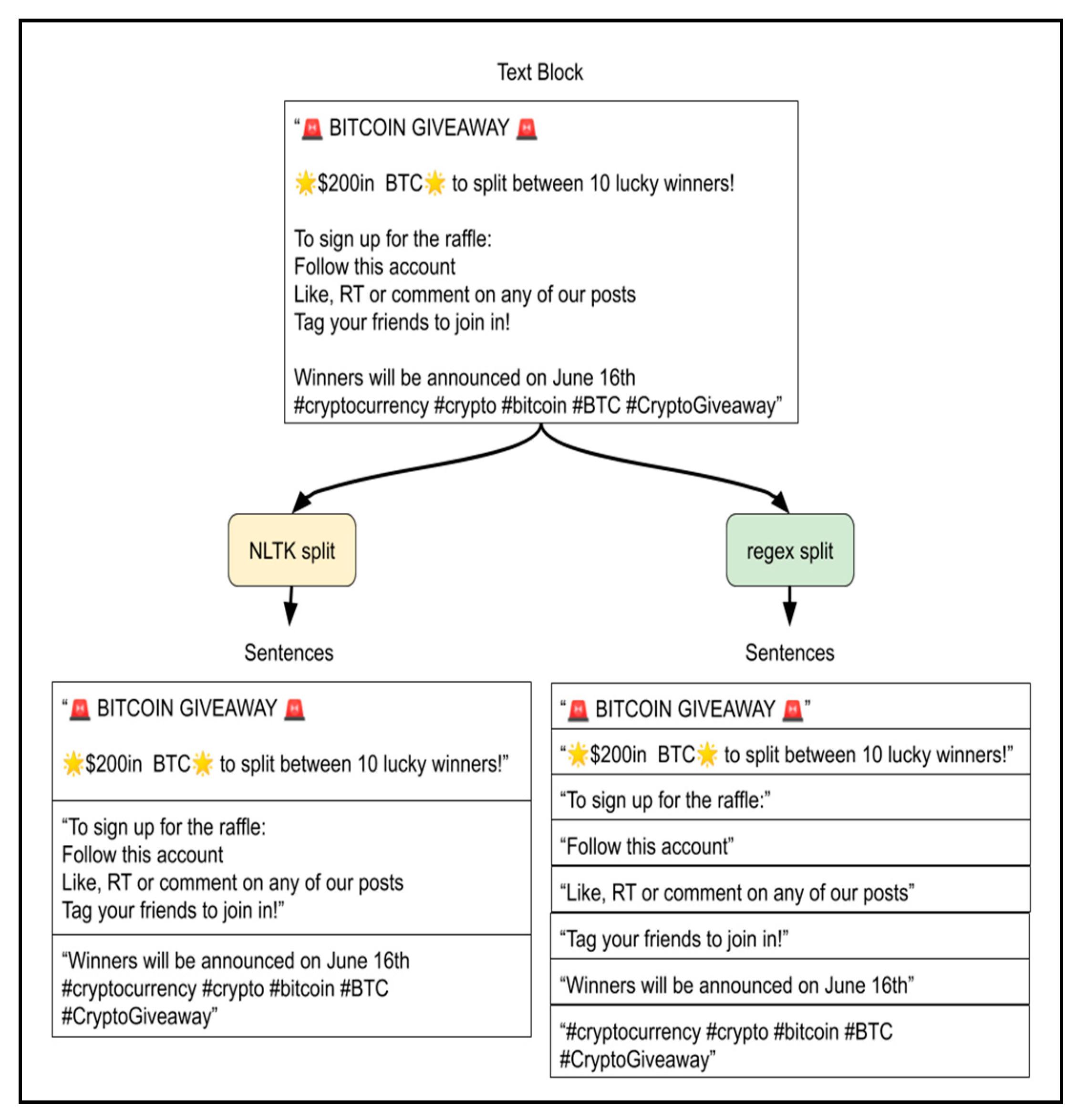
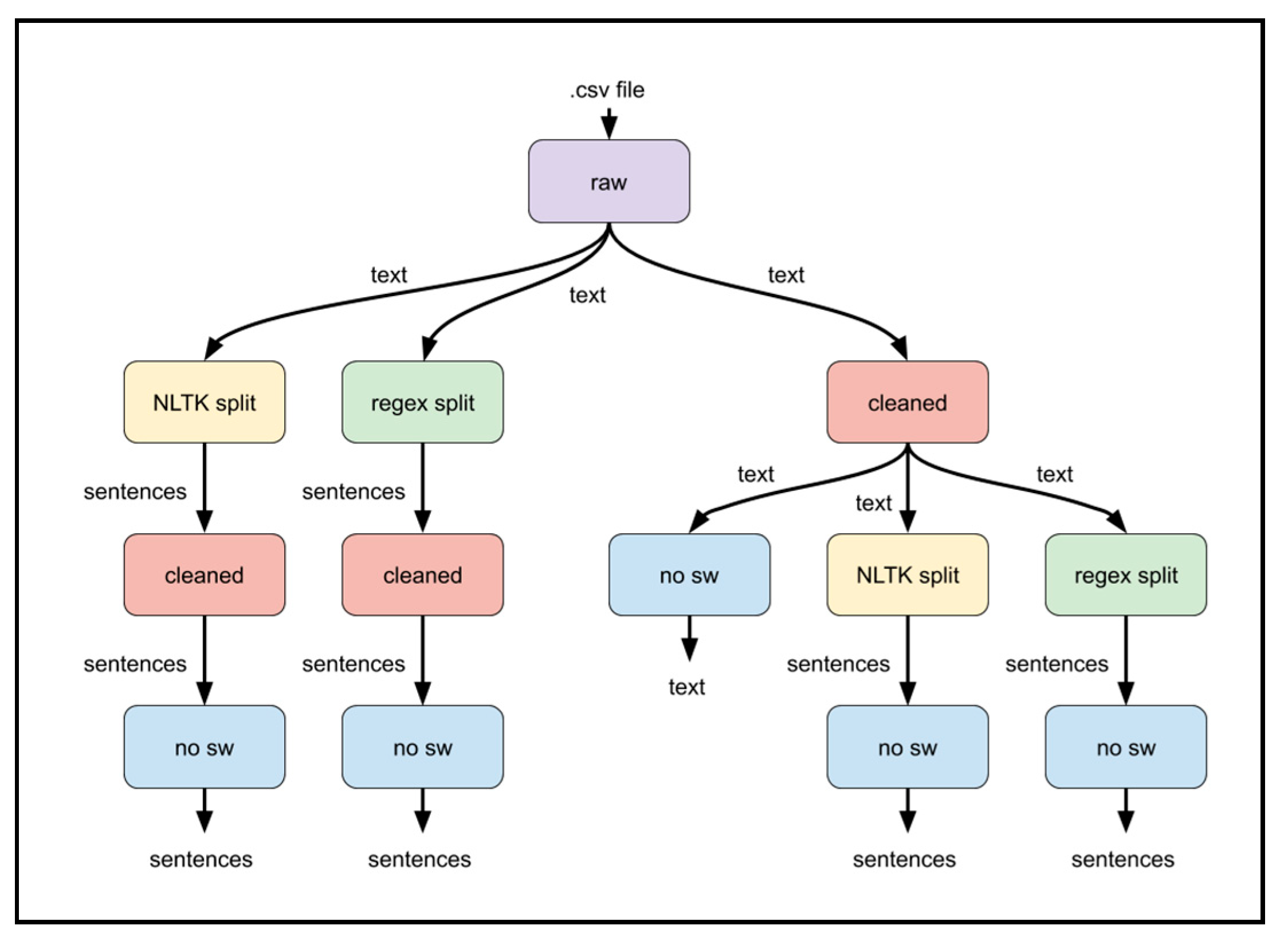
To determine whether certain preprocessing functions contribute to predicting Bitcoin prices, the output of those functions in various combinations was scored by VADER. All text cleaning functions of the preprocessing stage were combined in 5 different pathways. Scores of the text at intermediate steps of each path were recorded to determine if a function offers any improvement to the results. The “cleaned”, “NLTK split”, “regex split”, and “no sw” functions shown in
Figure 5 were combined to provide five different pathways. The “no sw” function was treated as the last step in any path, as no other function required word tokenization. Since VADER can be applied to a text of any length, the “cleaned”, “NLTK split”, and “regex split” functions produced a text of varying length. The “cleaned” and “split” functions were interchanged in different pathways. Both “split”, “cleaned”, and a “no sw” functions were applied afterward. The “cleaned” function can have either a “split” function used before the “no sw” stage. Our preprocessing combinations measured the scores of 13 intermediate steps (from 5 different pathways), as shown in
Figure 6. The text tweets and the preprocessed dataset are available for access and download in [
37].
4.4. Feature Types and Correlation
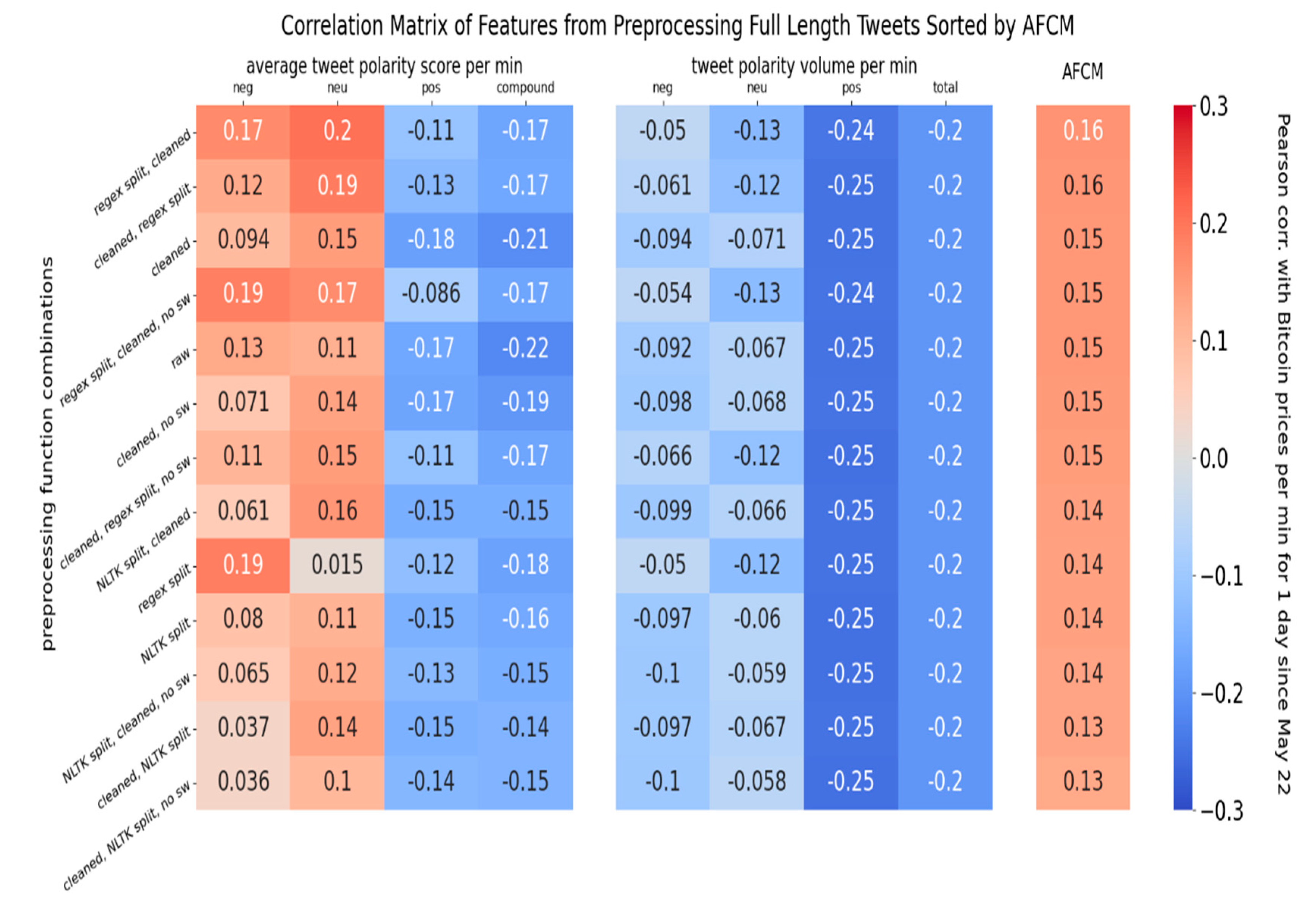
To account for differences in correlation due to the time length of the data used, we used subsets of data. The number of consecutive days of data varied and correlated with the respective Bitcoin prices occurring with the same timestamp. We will refer to this value as the correlation value of the subset. There are multiple unique subsets of data that span the same number of days. For example, a subset of 3 days of data can start on 22 May, 23 May, 24 May… 5 July, 6 July, and 7 July. Therefore, we averaged the correlation values from all unique subsets of data with the same length and differing start dates. The resultant value is independent of its start date (as much as it can be with a finite time length of collected data). Averaging the correlation values of all same-length subsets with different start dates should show us any correlation polarity (positive or negative) that a majority of subsets show. This is known as the Average Subset Correlation Polarity (ASCP, dashed line in figures). The correlation value could be positive, negative, or averaging; thus, we might hide how large the correlation values were and make the ASCP approach zero. To mitigate this effect, we can also average the absolute correlation values of all same-length subsets with different start dates to show the magnitude or strength of the correlation values. This is known as the Average Subset Correlation Magnitude (ASCM, solid line in all figures). The ASCP and ASCM are plotted as line graphs against the length of data in all subsets. The following eight figures show the ASCP and ASCM for common features produced from all 13 preprocessing strategies. A performance ranking scheme graph is included in those figures to rank each strategy from best to worst using the ASCM, for all subset data lengths. The 1st rank corresponds to the best performance and largest ASCM, while the 13th rank corresponds to the worst performance and smallest ASCM. The Pearson correlation average might not be a good representation of correlation magnitude if both positive and negative correlation values are averaged. Therefore, another experimental analysis using the absolute correlation value showing the average correlation magnitude per timespan length was conducted. For a total of 49.6 days of data, we measured all possible subset outcomes, and then we spanned contiguous days of data. Any subsets with the same timespan length and differing start dates had their outcomes averaged. This produced a time-series of correlation values for each of the cells in our correlation matrix.
We graphed the correlation time-series for all preprocessing strategies that share the same aggregation score type in the same figure to display this data.
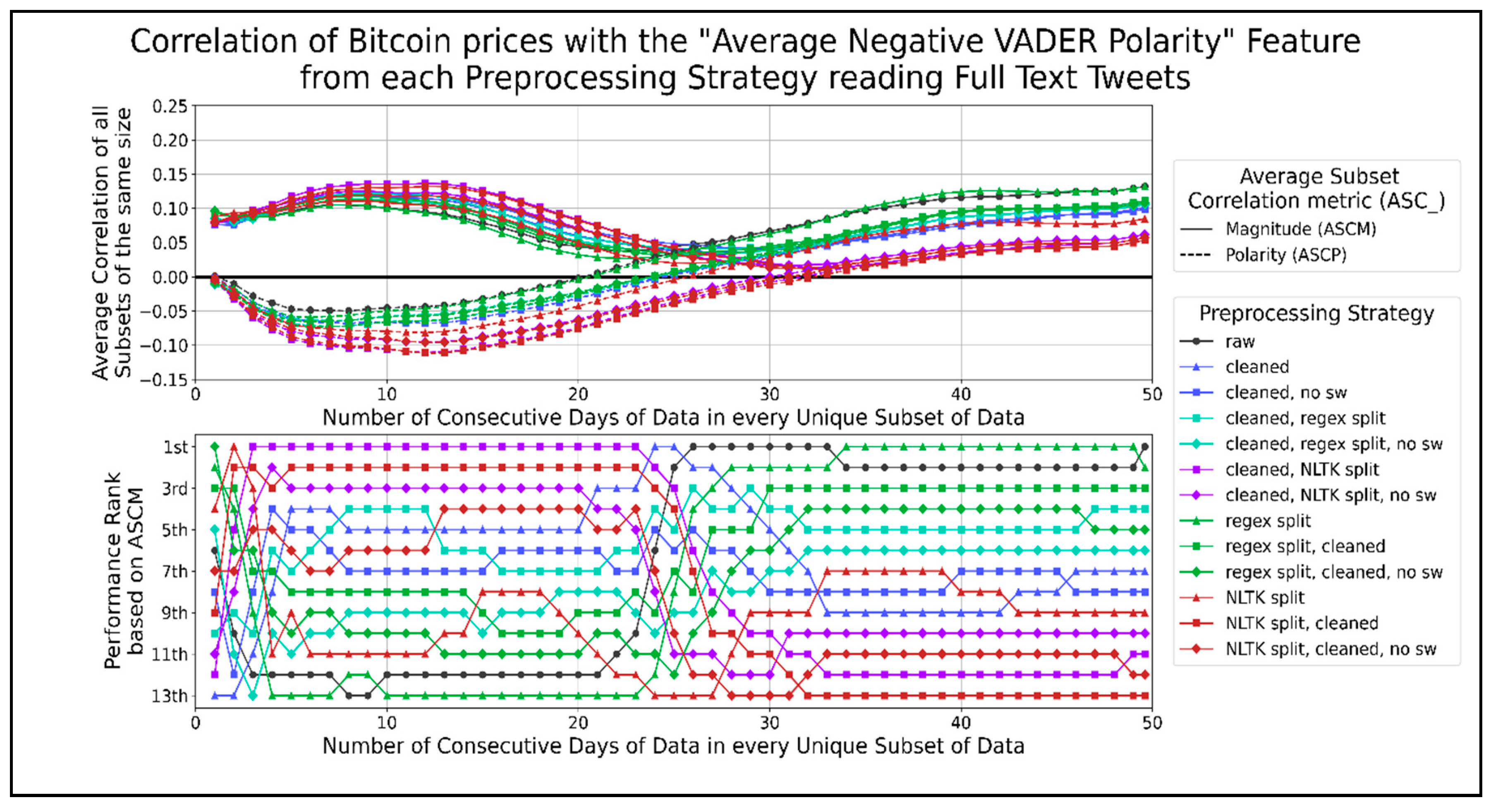
Figure 8 shows the trends for the correlation of average negative VADER sentiment with Bitcoin prices for different data timespans. Most preprocessing strategies performed better than raw text when using less than 20 days of data and show a negative ASCP. The top-performing strategies involve cleaning and splitting sentences using the NLTK library in any order before removing their stopwords. A general pattern of combining text cleaning and sentence splitting in any order had a higher correlation than removing stopwords from those combinations. Splitting sentences without being combined with other functions performed worse than the latter two combinations. However, this trend was reversed when using more than 20 days of data, as a positive ASCP developed. Splitting sentences on their own performed better than removing stopwords from any order of cleaned sentence splitting, which served better than any order of cleaned sentence splitting. Few preprocessing strategies performed consistently better than raw text, such as splitting sentences using a regex when using 35 to 45 days of data. Thus, the correlation of average negative VADER sentiments per minute showed opposite trends for datasets of different time lengths. The effectiveness of using any preprocessing strategy over raw text decreased as more days of data were used. Cleaning and splitting text in any order on 20 days of data or less seemed to work best, while splitting raw text into sentences using regexes worked best on more extended datasets. The most significant dip in the ASCP of −0.105 occurred when correlating 8 to 15 days of data. The largest peak in the ASCP of 0.123 occurred when correlating about 40 to 49.6 days of data.
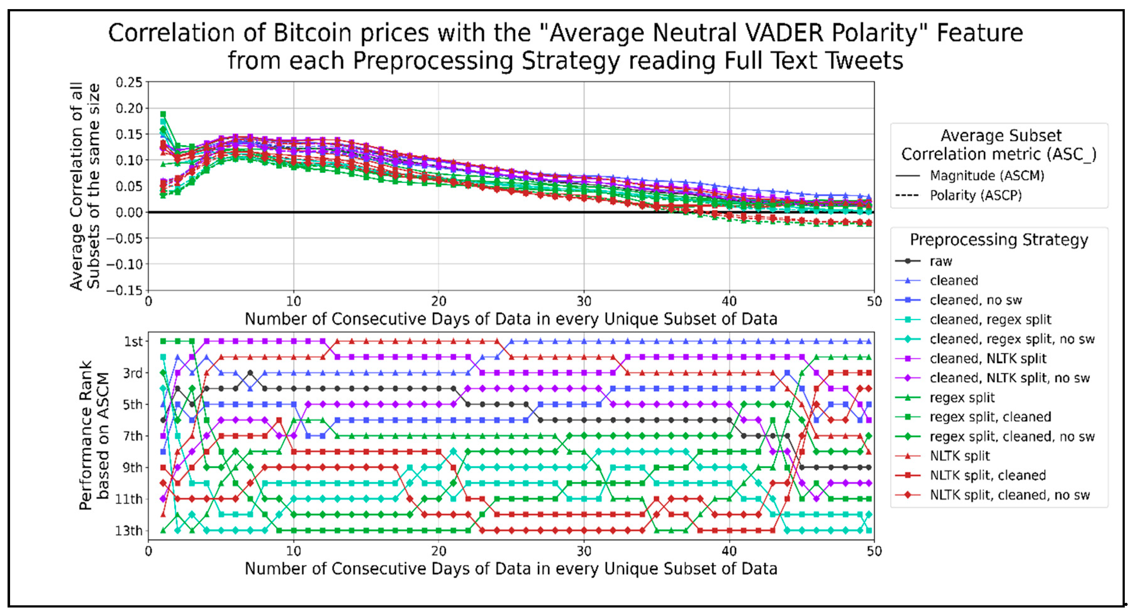
Figure 9 shows the correlation of average neutral VADER sentiment with Bitcoin prices over different data timespans. The only preprocessing strategies that consistently performed better than using raw text were cleaning text, splitting text into sentences with the NLTK library, and splitting sentences using NLTK after cleaning text. In general, combining NLTK split sentences with cleaning in any order reduced its ASCM, and removing stopwords from them reduced it further. Similarly, eliminating stopwords from cleaned text reduced its ASCM. The best performing preprocessing strategies for the average VADER neutral score per minute do not involve regex splitting or removing stopwords. The highest peak in both ASCP and ASCM for all strategies occurred when using about 6 to 13 days of data, excluding the rise for one day of data. This range showed a positive correlation of about 0.135.
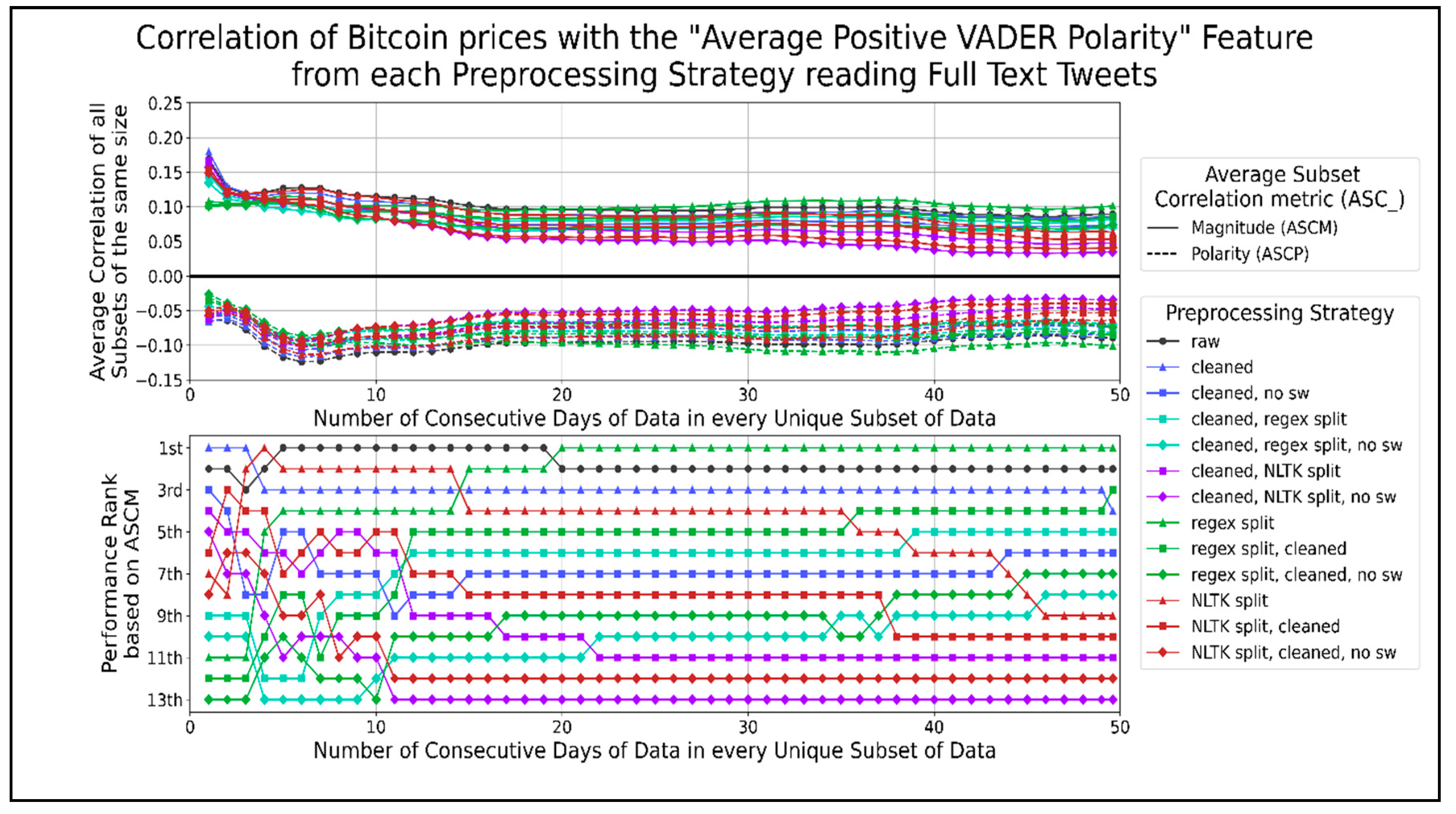
Figure 10 shows the correlation between average positive VADER sentiment with Bitcoin prices. Cleaning text outperformed when using 1 or 2 days of data. Splitting sentences by using a regex performed better when using more than 20 days of data. A general pattern of combining text splitting functions with cleaning reduced their ASCM, and removing stop words reduced them further. This indicates that the best performing preprocessing strategies for the average positive VADER sentiment per minute is raw text, followed by single functions (cleaning or sentence splitting on their own). The largest negative peaks in ASCP, of −0.12 and −0.10, occurred when using about 5 to 8 and 31 to 38 days of data, respectively.
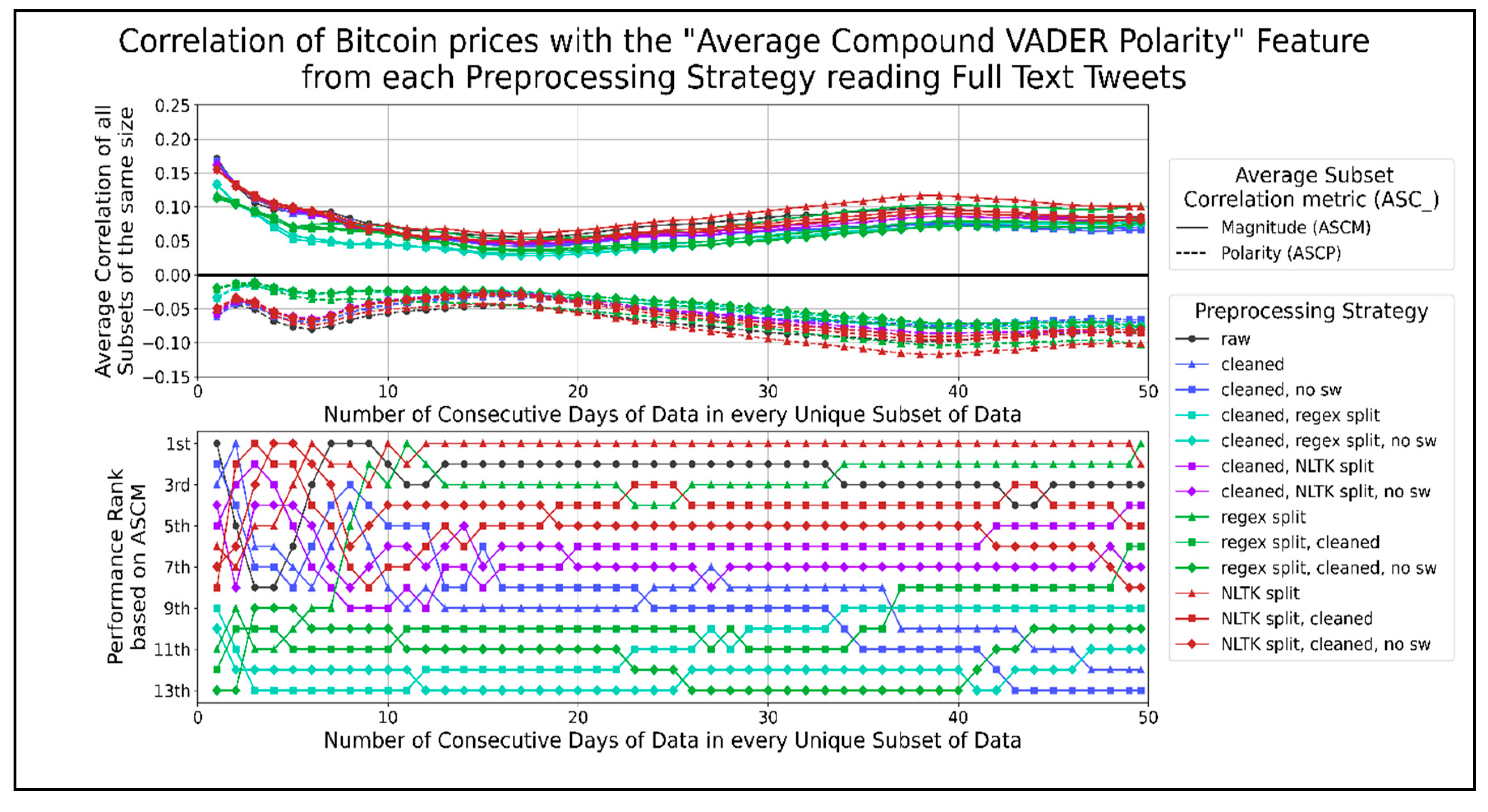
Figure 11 shows correlation graphs of the average compound VADER sentiment at different timespans for the Bitcoin prices. No preprocessing strategies have a consistently higher ASCM than raw text. However, a few preprocessing strategies perform well for a few data subset lengths. Cleaned text, splitting sentences using the NLTK library, and splitting sentences using a regex performed better than using raw text when 1, 19, or more, and 34 or more data days were correlated. In
Figure 11, in general, the best preprocessing strategies used the least amount of combined functions. Combinations of functions that split sentences using the NLTK library performed better than those using a regex. Therefore, the preprocessing strategies for the average compound VADER score per minute using raw text for less than 19 days of data and splitting sentences using the NLTK library for greater data lengths performed the best among other strategies. The largest negative peaks in ASCP were −0.06, −0.08, and −0.10 when correlating 1, 5 to 7, and 34 to 44 days of data, respectively.
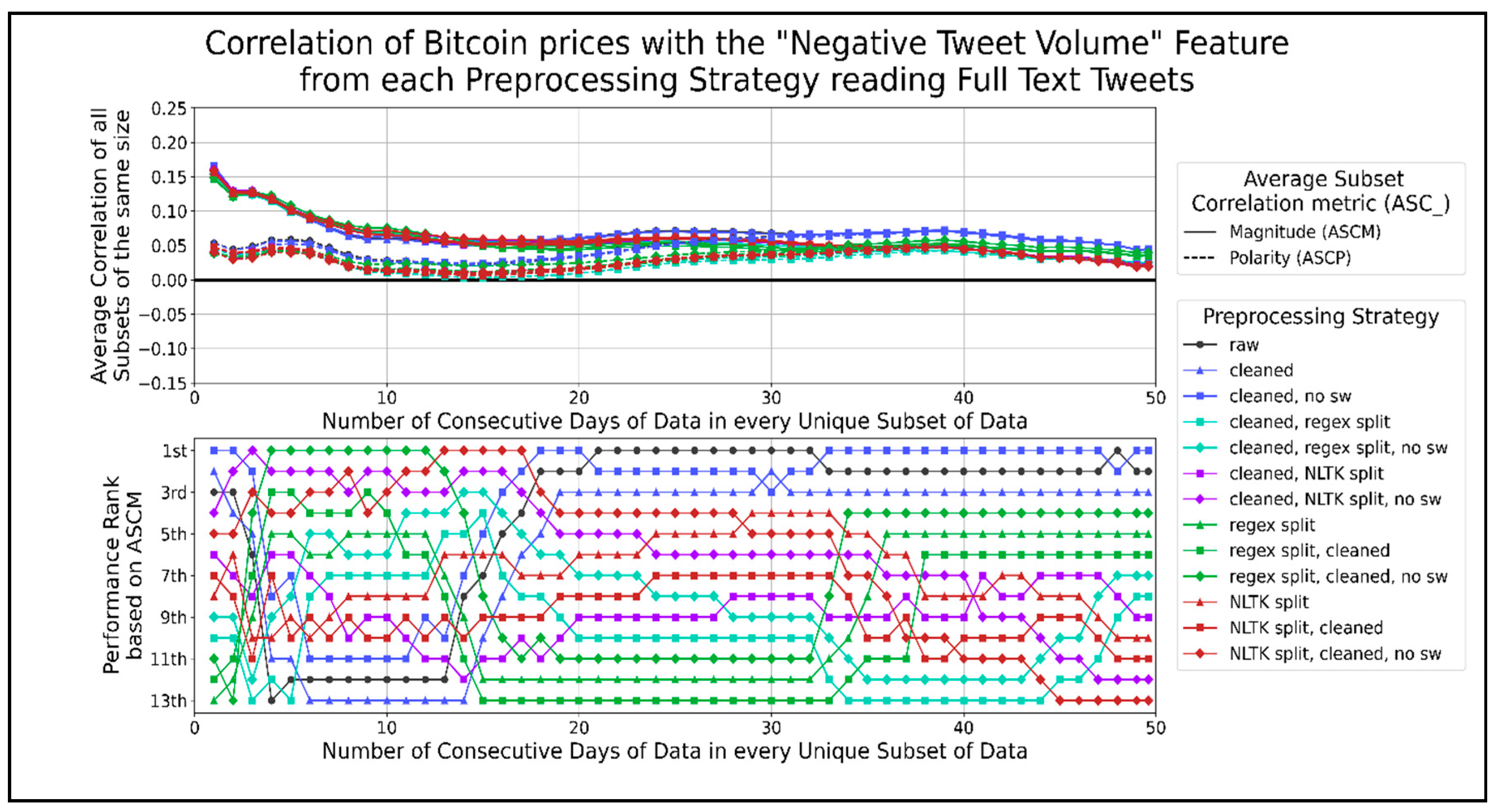
Figure 12 shows the correlation graphs of negative tweets per minute with Bitcoin prices. The cleaned text and cleaned text with stopwords removed closely match the raw text correlation. Cleaned text performed better than raw text when using between 35 days and 47 days of data, coinciding with the largest peak in the ASCP. A general pattern of sentence splitting combined with text cleaning, with stopwords removed, performed better than any sole sentence splitting method, which performed better than any order of combining sentence splitting and cleaned text. There was a large gap in performance between the three top strategies: raw text, cleaned text, cleaned text without stopwords, and the other preprocessing strategies. Therefore, the ASCM of the volume of negative tweets per minute was the highest when using those three strategies. The highest peak in ASCP was 0.07, at 40 days of data. Another peak of about 0.055 occurred when using 4 to 6 days of data.
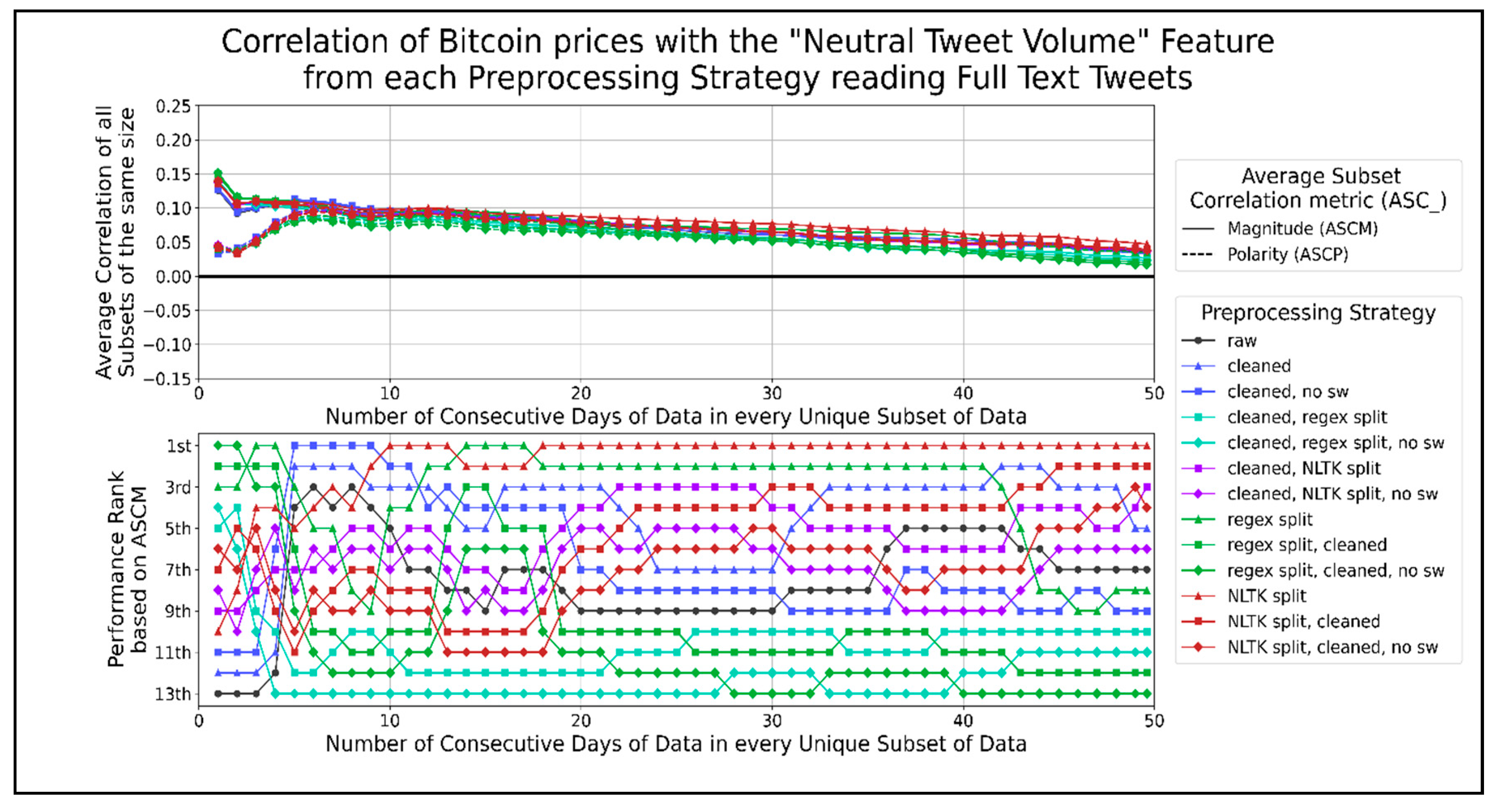
Figure 13 shows the correlation graphs of neutral tweets per minute for Bitcoin prices at different timespans. The top preprocessing strategies are splitting sentences using the NLTK library or a regex. In general, strategies that do not use a regex to split sentences tend to follow raw text correlation closely. Preprocessing strategies that use less combined functions achieve a higher ASCM than otherwise. Therefore, the preprocessing strategy that allows the volume of neutral tweets per minute, which correlates the best with Bitcoin prices, is the NLTK library to split sentences. The highest peak in ASCP was 0.095 when using 6 to 13 days of data.
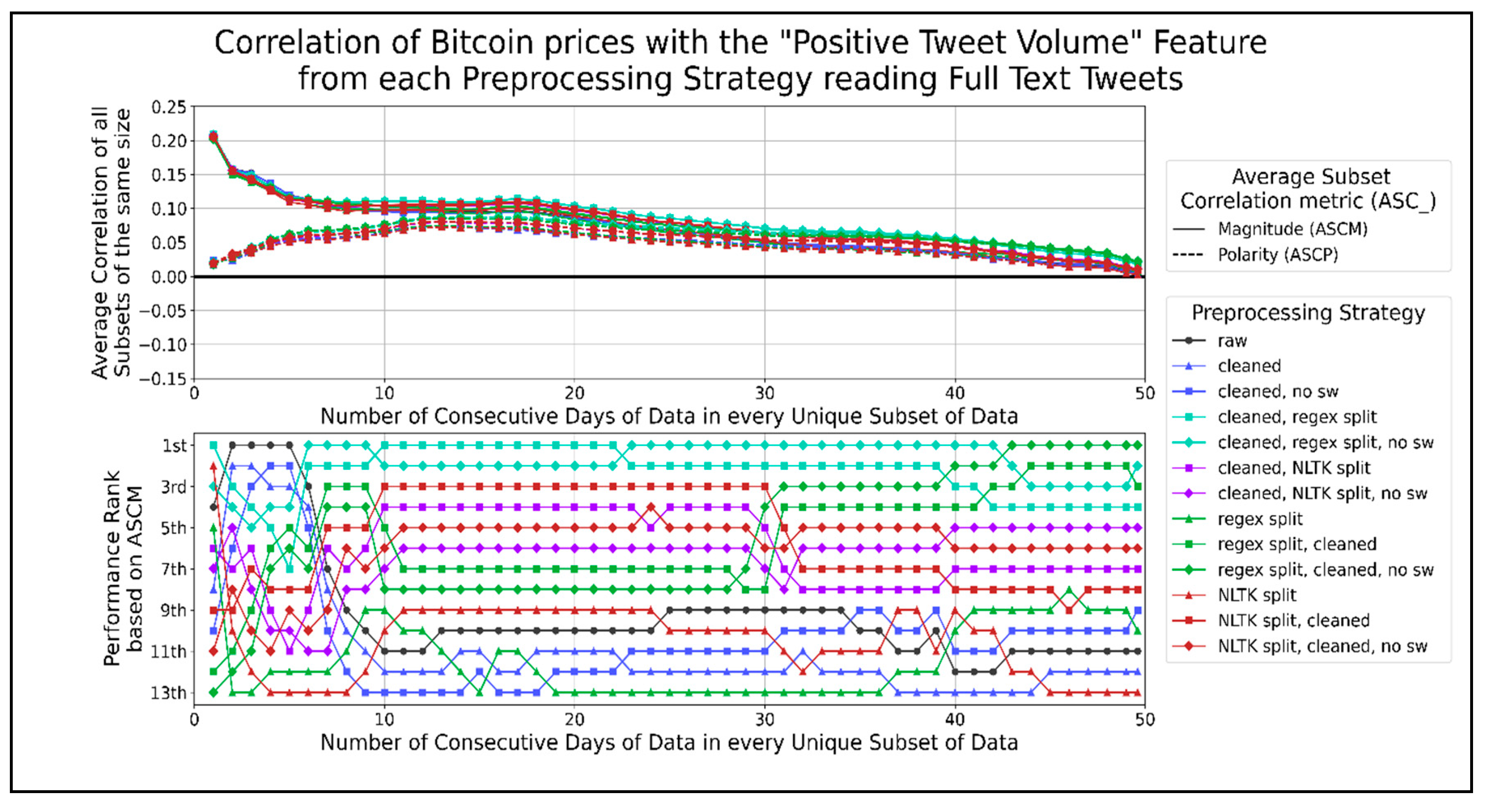
Figure 14 shows the correlation of positive tweets per minute with Bitcoin prices. The preprocessing strategies that consistently performed better than using raw text were the sentence splitting functions combined with one or more functions, such as cleaning text and/or removing stopwords. The top two strategies that performed the best involve cleaning text before using a regex for sentence splitting. In general, preprocessing strategies that involve combining more functions perform better. Therefore, the best preprocessing strategy for correlating Bitcoin prices with the volume of positive tweets per minute involves cleaning text before sentence splitting by a regex function. The highest peak in ASCP was about 0.085 when using 12 to 20 days of data.
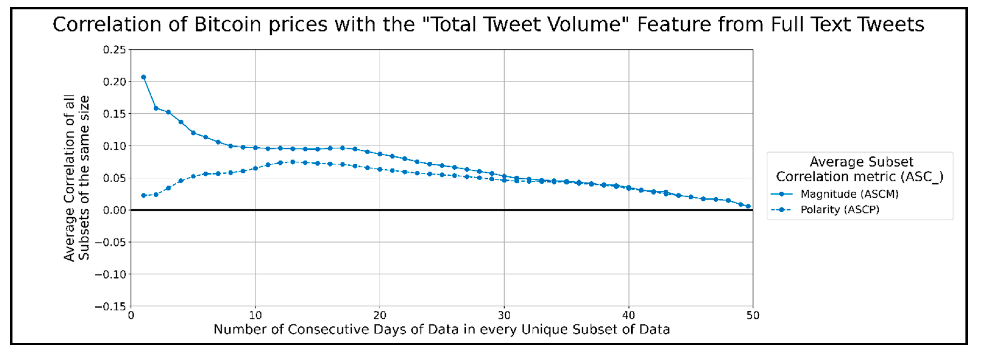
Figure 15 shows the total correlation per minute of tweets for Bitcoin prices. No preprocessing strategy can affect the total amount of tweets received from Twitter per minute; hence every single preprocessing function would have ASCM and ASCP graphs, as in
Figure 15. The highest peak in the ASCP was 0.09 and occurred when correlating 6 to 20 days of data.
It is worth noting that the correlation graphs of the total volume of tweets have a similar trend as the correlation graphs of the neutral and positive volumes of tweets. This may indicate that the correlation of the total volume of tweets shares more in common with the volumes of the neutral and positive tweets than negative tweets when using long-term datasets on a scale of days. The general trend of the above graphs shows the strongest correlation magnitude for shorter datasets of full-text tweet data and Bitcoin prices. When using one day of data for correlation, all ASCMs are significantly higher than when using all other timespans of data (except the average negative VADER scores per minute graphs). This could be a sign of sentiments expressed on Twitter, either responding to or anticipating a Bitcoin price change. However, the ASCPs, when using one day of data, are significantly lower than the respective ASCMs. This might show that any correlation observed with sentiments varies a lot depending on the date. We speculate that the substantial spike in correlation magnitude for a day of data on every graph indicates that correlation may become even stronger when observed on a shorter timescale, such as minutes instead of days. While there is no single preprocessing strategy that performs better than the rest for all feature types, we can see that cleaning text (and/or) splitting sentences is presented in most of the best strategies of each features. Any sentence splitting by itself seemed to work best for average VADER positive/neutral sentiment and neutral tweet volume, while NLTK splitting combined with cleaning worked best for average VADER neutral sentiment. Any sentence splitting also worked best for neutral tweet volume, while cleaning text worked best for negative tweet volume, and regex sentence splitting after cleaning text worked best for positive tweet volume. The feature types with the highest ASCMs around their highest peak were the positive/total tweet volume when a day of data was processed. No clear “best” features could be seen when all lengths of data subsets were considered. The highest ASCMs were all average VADER sentiments when less than 20 days of data were in each subset. ASCPs tended to show a second peak when processing 35 or more days of data to calculate the average VADER negative/positive/compound sentiments and negative tweet volume. These peaks may indicate longer-term data trends that continue outside of our 49.6 days of data, but they are typically low. However, they may be useful in machine learning algorithms that account for the past state, as recurrent neural networks.


