Weakly-Supervised Image Semantic Segmentation Based on Superpixel Region Merging

Abstract

In this paper, we propose a semantic segmentation method based on superpixel region merging and convolutional neural network (CNN), referred to as regional merging neural network (RMNN). Image annotation has always been an important role in weakly-supervised semantic segmentation. Most methods use manual labeling. In this paper, super-pixels with similar features are combined using the relationship between each pixel after super-pixel segmentation to form a plurality of super-pixel blocks. Rough predictions are generated by the fully convolutional networks (FCN) so that certain super-pixel blocks will be labeled. We perceive and find other positive areas in an iterative way through the marked areas. This reduces the feature extraction vector and reduces the data dimension due to super-pixels. The algorithm not only uses superpixel merging to narrow down the target’s range but also compensates for the lack of weakly-supervised semantic segmentation at the pixel level. In the training of the network, we use the method of region merging to improve the accuracy of contour recognition. Our extensive experiments demonstrated the effectiveness of the proposed method with the PASCAL VOC 2012 dataset. In particular, evaluation results show that the mean intersection over union (mIoU) score of our method reaches as high as 44.6%. Because the cavity convolution is in the pooled downsampling operation, it does not degrade the network’s receptive field, thereby ensuring the accuracy of image semantic segmentation. The findings of this work thus open the door to leveraging the dilated convolution to improve the recognition accuracy of small objects.

1. Introduction

In the last few years, convolutional neural networks [1,2,3,4] (CNN) have had widespread applications in various industries. The state-of-the-art semantic segmentation methods [5,6,7,8,9] rely on convolutional neural networks. Image-level marking plays a key role in segmentation. Because fully supervised [10,11] (pixel-level) semantic image segmentation is time-consuming and needs to be supported by high-performance CNNs, there is a lot of potential and challenges for weakly-supervised [12,13,14,15] semantic segmentation. For image semantic segmentation, there are two main methods: one is based on image-level labeling, and the other is image semantic segmentation based on pixel-level labels. Grangier et al. [13] implemented a semantic segmentation of images using a simple CNN model, which proved that CNN can achieve better results in semantic segmentation. However, it is time-consuming and laborious to label accurate marinade-level labels on a large amount of image data. Lin et al. [14] used scribble-supervised images to train a convolutional network for semantic segmentation. Dai et al. [15] used the bounding box to achieve the annotation of the target area, extract the feature information of the position and size of the image area to supervise the training of convolution networks. Liu et al. [16] used the depth features learned by CNN to establish a conditional random field (CRF) model [17,18,19] and used the structured support vector machine (SSVM) to learn the CRF model parameters, avoiding the manual extraction of image features.

The feature representation of images is a key step for image semantic segmentation. The feature-based work includes: a random forest-based classifier [20], TextonForest [21]. Yan et al. [22] proposed a model for assigning labels to super-pixels by learning related features, which are used to merge superpixel blocks to extract candidate regions. Liu et al. [23] proposed a weakly-supervised method based on graph propagation, which automatically assigns image-level labels to the super-pixel context information. Aminpour and Razzaghi [24] used a two-layer graphical model to assign labels to super-pixels by linking local and global similarity features for weakly-supervised semantic segmentation. These methods all study the model on superpixel segmentation. It is well known that super-pixels can be described in detail for local structures, so their application in the framework of convolutional networks is increasing. Zhang et al. [25] used the local detail optimization of super-pixels, the mean field inference algorithm, and the quadratic programming relaxation correlation algorithm to optimize the CRF in order to obtain the final label assignment result. Hence, the superpixel method for graphic preprocessing is used frequently. However, improving the performance of super-pixels in weakly-supervised semantic segmentation will be the focus of this work.

Furthermore, transfer learning [26] continues to be a popular learning framework because it enables training CNN with a relatively small dataset. Oquab et al. [27] utilized a simple transfer learning procedure to demonstrate how image representations learned with CNNs on large-scale annotated datasets can be efficiently transferred to other visual recognition tasks with a limited amount of training data to achieve state-of-the-art results. Also, Jiang et al. [28] used transfer learning to scale down the disparity in data distribution between training and test data. Şeker [29] used transfer learning to overcome the large number of data markers required by deep learning algorithms. Hence, due to the small size of the PASCAL VOC 2012 [30] dataset used in this work, we will also use transfer learning to train our network.

According to theoretical hypothesis [25,31], we present an image semantic segmentation method based on superpixel region merger and CNN. At the same time, a series of linear constraints are incorporated into the training process to improve recognition of the target’s contour. Furthermore, because manual labeling is very time-consuming on a large number of data sets, we employ a superpixel segmentation theory and combine the superpixel regions to form larger superpixel blocks based on the region adjacency map to achieve the same labeling effect. Compared to the pixel level annotation [8], the pixel block provides the pixel information of the region, which should have a good effect. Also, compared to the scribble-supervised approach [14], in the manual annotation, time is saved.

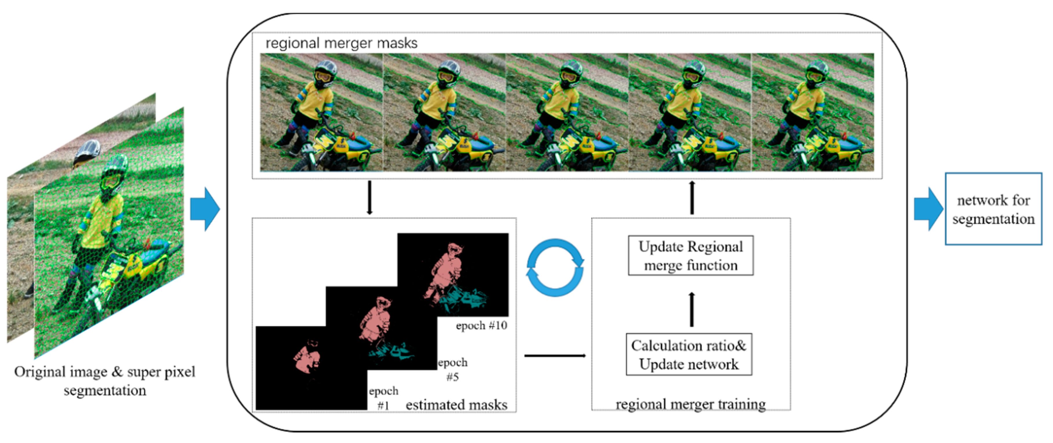
The proposed approach works as follows: Firstly, the original image is subjected to simple linear iterative clustering (SLIC) superpixel segmentation [32,33], and then three criteria (i.e., full lambda, spectral histogram or color-texture model) are used for super-pixel region merging. The merging is also the makeup of the pixel block. After merging, we can obtain a set of target areas that have already been marked. We then used a graphical model to supervise the merged marker areas and produce predictive results. Furthermore, a loss function is used to calculate whether the result is expected. Then, we feed the results back to the optimization function and optimize the process of the previous step which includes parameter adjustment of the region merged and supervision training for unmarked pixels. Merging the graph model again will propagate the spatially constrained block of pixels to the unlabeled block of pixels. Simultaneous use of a full convolutional network (FCN) provides a semantic prediction for graphical models, although the output is rough at the outset. However, we use an iterative-feedback mechanism to optimize the graphical model, feedback the predicted value to the optimization function, and update the pixel combination to achieve the optimal result. All these steps are illustrated in Figure 1.

Figure 1. The flow chart of supervision training based on regional merging neural network (RMNN).

In the remainder of this paper, we introduce the preprocessing SLIC for superpixel region merging and transfer learning of visual geometry group 16 layers (VGG16) related theory in Section 2. We provide the details of regional merging neural network (RMNN) in Section 3. Section 4 presents our experimental results. Finally, we conclude this paper with future directions of research in Section 5.

2. Related Work

In computer vision, super-pixel refers to irregular pixel blocks with certain visual significance composed of adjacent pixels with similar texture, color, brightness, and other characteristics. It groups pixels with similar characteristics and describes the image with a small number of pixel blocks instead of a large number of pixels. In this way, the computational cost of image preprocessing and the complexity of the algorithm can be greatly reduced. Hence, super-pixels are frequently used as the preprocessing step in image segmentation.

Weakly-supervised image semantic segmentation is the use of image-level annotations to try to capture all the positive factors. However, the main problem is how to divide the image into many different regions. Zhao et al. [31] proposed a simple linear iterative clustering method based on boundary terms (BSLIC) and semantic segmentation combined with full convolutional networks (FCN). They achieved an improvement in the segmentation algorithm by introducing superpixel semantic annotation. In this paper, we have also adopted the simple linear iterative clustering (SLIC) algorithm, which is widely used today. The aggregated pixels are considered as positive factors. We use images with merged regions to train the complete convolution network.

The BoxSup-based [15] semantic segmentation method uses artificially labeled bounding box annotations as an alternative or external source of supervision to train convolutional networks for semantic segmentation. The advantage of our approach is that it avoids human intervention and uses superpixel merging as an automatic annotation method.

Our algorithm solves two problems. The first problem is the automatic labeling of images. We use the region formed by superpixel fusion as a boundary line annotation and an external monitoring source for convolutional network training for semantic segmentation. This contrasts with Lin et al. [14] who employed manual marking of images, which requires user interactions and can take more time to complete. Hence, the advantage of our proposed superpixel merging method is that the image is automatically annotated, and the target can be annotated in the form of a bounding box, which saves annotation time. Through experiments on the super-pixel region merging method, we found that it took 0.172 s on average. Therefore, applying superpixel segmentation to the architecture increases the computational cost.

The second problem is the optimization of image contour recognition. SLIC can quickly and efficiently form super-pixels with nearly uniform density and rich edge information. We found that the size of the fused regions varied, and the mask mold at the beginning was very rough. We first use small area training, then provided useful information for the network, and then merged these small areas for supervisory training. So, the outline of the image was gradually improved, and the two tasks were performed in an iterative manner.

2.1. Transfer Learning of Visual Geometry Group 16 Layers (VGG16)

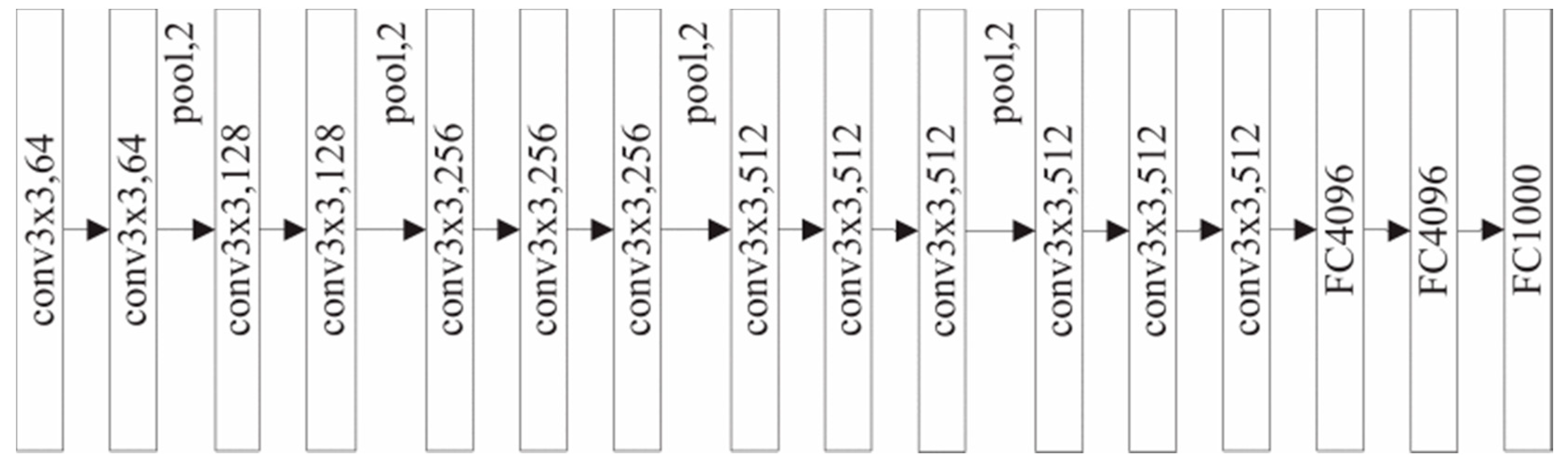
The input to VGG16 is an RGB image of 224 × 224, and it uses three 3 × 3 convolution kernels instead of the previous 7 × 7 core to extract features (Figure 2). This can reduce the complexity of training, but not the accuracy. On the other hand, the decision function can be made more competitive because three correction layers are used instead of one correction layer. Compared to VGG19, VGG16 has fewer training layers and does not reduce the intersection over union (IoU) value. Therefore, considering the superior performance of VGG16, it is used as a feature extraction model in this paper.

Figure 2. Structure diagram of Visual Geometry Group 16 layers (VGG16).

Transfer learning [27] can be pre-trained on large data sets (such as ImageNet), and then transfer the trained network weights to a small data set, that is, fine-tuning the network with a small data set, so that the network can be applied to small data set. Moreover, the CNN middle layer can be regarded as an extractor of image representation, pre-trained in the original ImageNet data set, and applied to our experimental data set, PASCAL VOC 2012 [30]. The main objective is to correctly classify and identify the target T in a domain P. Moreover, the role of migration, or transfer learning, is to improve the classification results of the objective function ε(θ) in the domain. However, due to the identification of targets in different domains or fields, different migration learning models exist. Transfer learning is a class of induction, so it is more applicable to unsupervised or weakly-supervised learning. In this work, we leveraged the VGG16 model as shown in Section 3.2 and replaced the last 1000 classes with our 21 classes. In addition, for fine-scaled image edges and details, we initialized the last layer with Gaussian noise.

2.2. Objective Function

Our superpixel region merging method is applicable to many existing CNN-based mask semantic segmentations, such as EM-Adapt [12], BoxSup [15], and other variants [34,35]. In this article, we adopt the FCN model that has been improved by CRF as a mask supervision baseline. Our constraint is to transfer the superpixel tag to a zone tag. Three conditions should be met: (1) The image contains at least one super pixel label, (2) There can only be one label in a region, (3) The label $X_{\theta }$ of the area should be a super pixel set having the same label. Our goal is to superimpose the merged area as a superimposed model in such a way that the FCN’s network training becomes the superpixel regression problem of the ground-based segmentation model [15]. The objective function (1) is:

$$\mathsf{\epsilon }\left(\theta \right)={\displaystyle \sum }_{b}e\left(X_{\theta }\left(b\right),l\left(b\right)\right)$$

(1)

where $b$ represents the pixel index, $l\left(b\right)$ is the ground truth value semantic label of the pixel, $X_{\theta }\left(b\right)$ represents the pixel label produced by a fully convolutional network of parameter ($\theta$), and $e\left(X_{\theta }\left(b\right),l\left(b\right)\right)$ is a pixel loss function. The CRF is used as a post-processing FCN result.

2.3. Simple Linear Iterative Clustering (SLIC)

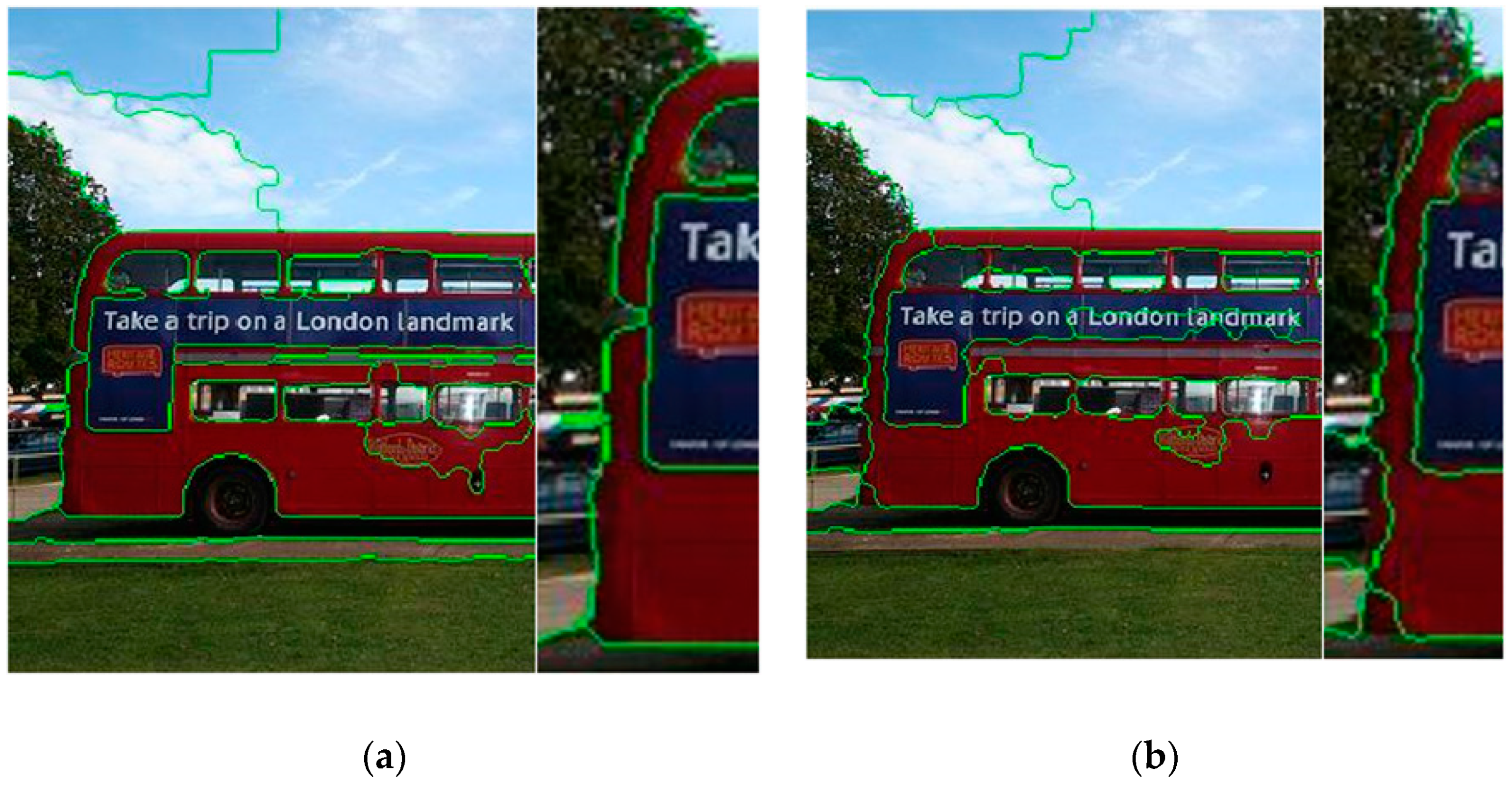
The SLIC algorithm uses the same similarity parameter for the pixels in the image, which can be set by the user. The problem with SLIC is that all areas of the image are both smooth and highly textured. SLIC generates a regular sized super-pixel in the smooth areas while it generates an irregular super-pixel in the highly textured regions. An improved version of SLIC, namely zero parameter version of SLIC (SLICO), solves the whole problem thoroughly, producing regular super pixels in both areas. Also, the speed of the iterative segmentation phase of the algorithm is greatly improved. However, in this work, we chose SLIC instead of SLICO. Although the super-pixels that SLICO produces are regular, the pixels in many regular sizes do not have the same characteristics. Hence, it is worse than SLIC when combined with super-pixels. Figure 3 shows the difference between the two methods.

Figure 3. The region merge graph of Simple Linear Iterative Clustering (SLIC) and zero parameter version of SLIC (SLICO). (a) is the magnified regions of SLIC, (b) is the magnified regions of SLICO. The figure shows the effect of boundary term.

We examined the boundaries of the image by examining the gradient values of the pixels by the boundary terms, by comparing the merged boundaries of the two methods in Figure 3. The edge of the superpixel in (a) is better adhered to the object boundary in the image. Based on the super-pixels on the image boundary, it is possible to calculate whether the edge of the superpixel is aligned with the object boundary in the image according to the boundary term formula [36]. When the edge of the superpixel is aligned with the boundary of the object in the image, the algorithm is more advantageous. When using the boundary recall (BR) as a measurement, SLIC can achieve 61.26% accuracy, which is 4.21% higher than SLICO.

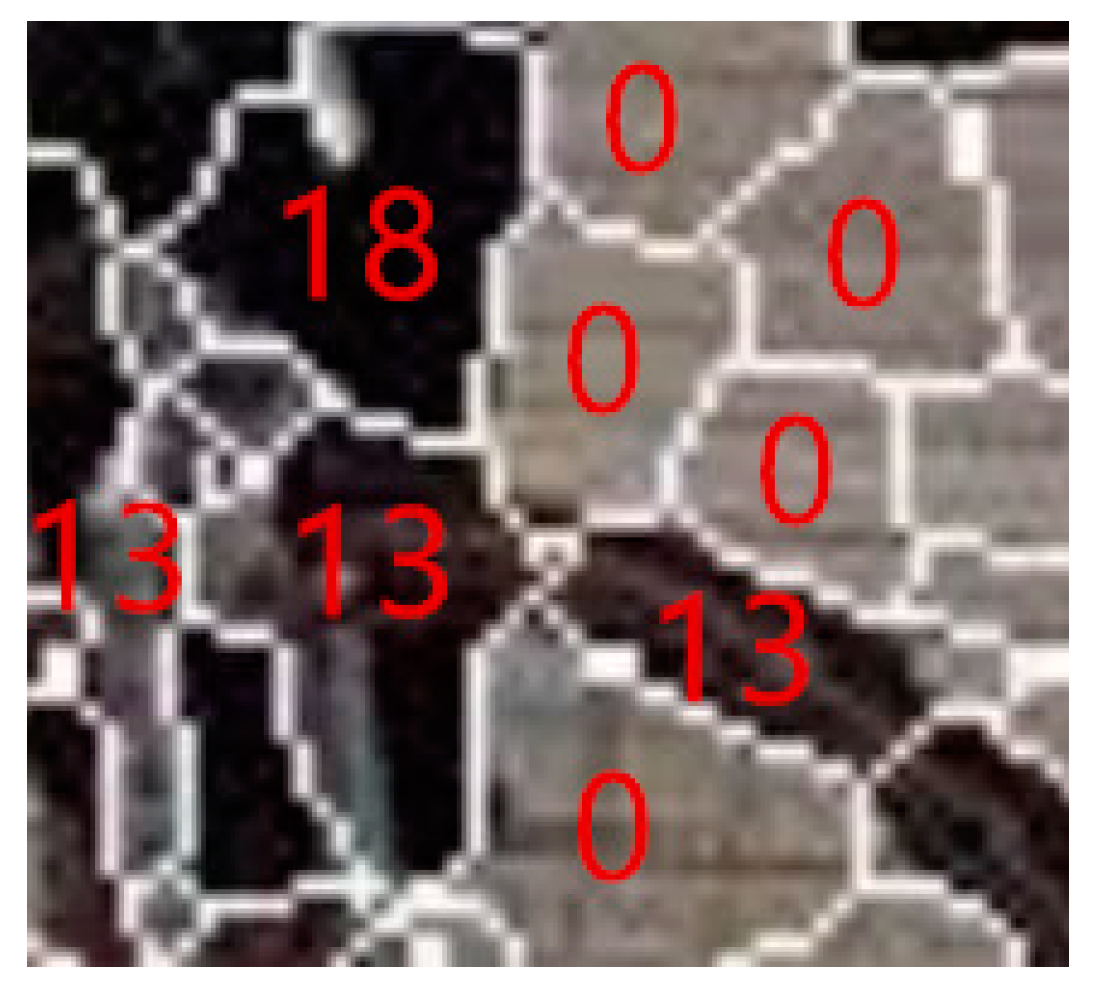
2.4. Superpixel Annotation

The SLIC annotation algorithm is described for each seed point of a superpixel, that can be described as $[C_i=\left(L_i,A_i,B_i,x_i,y_i,sig{n}_i\right)]$, where we use the color characteristics of the CIELAB color space $\left(L,A,B\right)$ and location information. $sig{n}_i$ denotes the annotation information of the super pixel. Figure 4 shows an illustration.

Figure 4. Superpixel semantic annotation information. The area consisting of white lines is produced by superpixel segmentation, while the red numbers represent the semantic labels of each region.

Suppose the image contains N pixels, and we pre-split k kinds of super-pixels of the same size and each grid width is $S=\sqrt{N/k}$. The seed point $C_i$ is initialized by the grid with the step size S. Then, we calculate the similarity between the pixel point and the seed point within the neighborhood of $2S\times 2S$ for each seed point $C_i$ and the pixel with high similarity is allocated (Formula (2)). The background category, $sig{n}_i$ is also initialized. Furthermore, we iteratively recalculate the seed points until convergence.

$$D=\left|\left|I-I_k\right|\right|+m\sqrt{{\left(x-x_k\right)}^2+{\left(y-y_k\right)}^2}/s$$

(2)

where $I_k$ and $I$ represent the pixel intensity of the seed point and nearby pixels, $x_k$ and $y_k$ represent the vertical seed point and horizontal coordinate values, where $x,y$ represent the vertical and horizontal coordinate values of the nearby pixel points and $S$ represents the distance between the seed points. m is used to measure the relationship between the intensity of the pixels and the spatial information in the similarity calculation.

3. Regional Merger Algorithm

3.1. Regional Merger

In the SLIC method, when the number of super-pixels divided is larger, the accuracy of segmentation of the object can be increased when the regions are merged. Hence, we iteratively merged those very small super pixels. By the region merging method, the image segmentation accuracy has been promoted and the high-precision boundary from the initial partition is preserved.

The fast and effective approach in our proposed region merging algorithm is to model the image as a region adjacency graph (RAG) [37]. Each super-pixel region is regarded as a point in the graph. When two regions are adjacent, the corresponding nodes are connected by edges with the same weight and the merging of the regions is realized by merging the nodes in the graph. In order to merge regions at a minimum cost, we have three criteria representing different features (i.e., shape, spectrum, texture) to calculate the difference caused by the image approximation problem and how it affects the cost of the merge. λ is the parameter of the three criteria.

• Merging criterion 1, Full Lambda:

  $$\{\begin{array}{c}{C}_{i,j}=\frac{C_i·C_j}{C_i+C_j}h\left(i,j\right)\\ h\left(i,j\right)={\left({\mu }_i-{\mu }_j\right)}^2·\frac{1}{l^{\lambda }}\end{array}$$

  (3)

  where $C_i$ is the area, ${\mu }_i$ is the mean spectral value, $l$ is the shared boundary of region $i \mathrm{and} j,\mathrm{and} \lambda$ is the shape parameter.
• Merging criterion 2, Spectral Histogram [38]:

  $$\{\begin{array}{c}{C}_{i,j}=\frac{C_i·C_j}{C_i+C_j}h\left(i,j\right)\\ h\left(i,j\right)=G\left(i,j\right)·\frac{1}{l^{\lambda }}\\ G\left(i,j\right)=2\left({\displaystyle {\displaystyle \sum }_{i,j}}{\displaystyle {\displaystyle \sum }_{i=1}^t}{f}_i\log f_i-{\displaystyle {\displaystyle \sum }_{i=1}^t}\left({\displaystyle {\displaystyle \sum }_{i,j}}{f}_i\right)\log \left({\displaystyle {\displaystyle \sum }_{i,j}}{f}_i\right)+1.3863\right)\end{array}$$

  (4)

  where $G\left(i,j\right)$ is the G-Statistic value of two spectral histograms i and j, $f_i$ represents the probability density function.
• Merging criterion 3, Color-Texture Model [39]:

  $$\{\begin{array}{c}{C}_{i,j}=\frac{C_i·C_j}{C_i+C_j}h\left(i,j\right)\\ h\left(i,j\right)=\left(w_C{G}_c+w_T{G}_t\right)·\frac{1}{l^{\lambda }}\\ G_c=\frac{1}{D}{\displaystyle {\displaystyle \sum }_{a=1}^D}{G}_C^a\left(i,j\right)\end{array}$$

  (5)

  where $Gc$ is the G-Statistic value of two spectral histograms, D represents the number of bands of the image with a value of 0.30–0.76 (µm), $G_C^a\left(i,j\right)$ represents the histogram distance of the regions i and j in the a-th band. $G_t=G\left(i,j\right)$ is the G-Statistic value of two LBP texture histograms; $w_C$ and $w_T$ are the corresponding weights (these two values are automatically estimated). $C_{i,j}$ is expressed as the combined value of the region $\left(i,j\right)$, and $\left(i,j\right)$ represents the heterogeneity of the two regions. $l$ is the shared boundary length of the adjacent region $\left(i,j\right)$; $\lambda$ is the influence coefficient of the boundary. When the parameter $\lambda =0,l^{\lambda }=1$, indicating that the boundary does not affect the regional heterogeneity metric. On the other hand, if $\lambda \ne 0$, indicating that the longer the boundary, the smaller the heterogeneity.

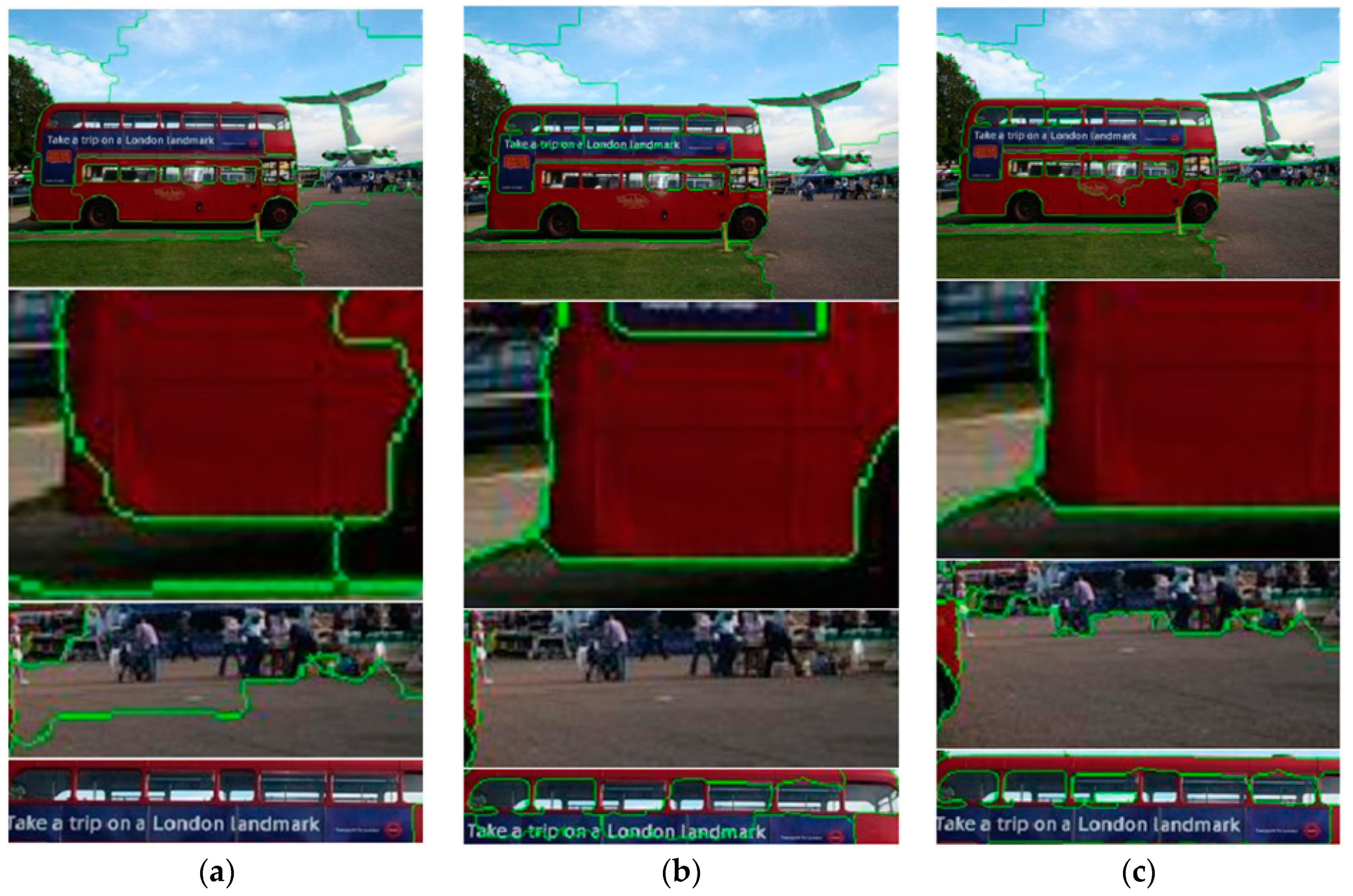
Figure 5 shows the segmentation results obtained by the region merging algorithm adopting different criterion and some details of the show. It can be seen that the average intensity of the pixel’s color area reflects the local pixel color features, and the pixel is obtained by clustering the consistency of the characteristics of the local area. Therefore, the mean intensity of the color is very important. It can also be seen from Figure 5 that the best aggregation result was obtained by criterion 3. Through fusion, we obtained the relatively complete edge information and the background also achieves a certain degree of aggregation. We evaluated the segmentation results experimentally. The BR values of the three criteria are 59.24%, 92.71%, and 63.15%, respectively, which justifies that the third criterion is better in performance.

Figure 5. A merged graph when different criteria are used. The values of (a–c) represent the results of criteria 1, 2, and 3. In terms of detail, the third image works better. Therefore, criterion 3 was chosen as the consolidation criteria.

The super-pixel region fusion (Algorithm 1) was performed on the original image. However, because the target in the original image has color information, the super-pixel image segmentation will be used to improve the accuracy of the edge obtained. After the SLIC superpixel segmentation, we obtained a cluster $\mathrm{C}=\left\{C_1,C_2,\cdots ,C_k\right\}$ with similar size area and each pixel has a pixel label, which is expressed as $C_i=\left(x_i,y_i,sig{n}_i\right)$, where $\left(x_i,y_i\right)$ is the pixel coordinate information in area $C_i$, and $sig{n}_i$ is the super-pixel inner label.

Algorithm 1. Superpixel region merging

1.  We initialize the image by using the step size s to obtain the cluster center set $\mathrm{C}=\left\{C_1,C_2,\cdots ,C_k\right\}$.

2.  Move the clustering point to the position with the smallest gradient in 3 * 3.

3.  Set the label $sig{n}_i=-1$, and the distance $d_i=\infty$ for each pixel i.

4.  Iterate over the points in the collection:

5.  For each cluster center $C_i$:  For each pixel i in a 2s × 2s area around $C_i$   Calculate the distance D between $C_i$ and i   if $D<d_i$ then    set $d_i=D\&sig{n}_i=i$   end if   Add $C_i$ to collection C.  End for End for

6.  According to steps 1 through 5, cluster $\mathrm{C}=\left\{C_1,C_2,\cdots ,C_k\right\}$ is obtained.

7.  Calculate the color (spectral) intensity mean ${\mu }_j$ (criterion 1) of the pixel in each super pixel cluster $\left(C_i\right)$.

8.  Iterate through the super-pixels in C and select the super pixel $C_i$ in set C as the starting point in turn and mark the point has been accessed.

9.  Search for the neighborhood superpixel of $C_0$ and find all adjacent super-pixels ($C_n$). The adjacent super-pixel pair $P_{0n}\left(C_0,C_n\right)$ is composed, and represent all the super-pixel sets of the $C_0$ neighborhood as $\mathrm{neighbors}=\left\{\left(C_0,C_{n1}\right),\left(C_0,C_{n2}\right),\cdots ,\left(C_0,C_{nk}\right)\right\}$, where k is the number of neighborhood super-pixels.

10.  Start with the selection of criterion 3 when the area of the super pixel pair $(\frac{C_i·C_j}{C_i+C_j})$ is small, i.e., it has a priority merge right (In the case where the regional heterogeneity is the same, the smaller the area of the region, the smaller the error caused by the merger for the entire image approximation). Furthermore, when the area of each pixel pair is similar, calculate and compare the heterogeneity $\mathsf{\delta }=h\left(i,j\right)$ of each adjacent superpixel pair $\left(C_0,C_n\right)$ to determine whether to fuse. When $\mathsf{\delta }$ is minimum, the fusion condition is satisfied. Otherwise, fusion is not performed.

11.  If the super pixel pair is fused, the pixel label in the fused cluster is updated to $sing{n}_{C_0}=sing{n}_{C_n}$. Also, the edge weight of $h\left(i,j\right)$ is updated and the pixel point $C_n$ is marked accessed. If no fusion is performed, no processing is performed.

12.  Traverse the neighborhood collection neighbors. If $C_n$ in $P_{0n}\left(C_0,C_n\right)$ has been marked accessed, merging is performed and $sing{n}_{C_0}=sing{n}_{C_n}$. Otherwise, do not process.

13.  Repeat steps 7 through 12 until all super-pixels have been accessed.

14.  The fusion is completed, and the new clusters are obtained.

3.2. Algorithm Framework

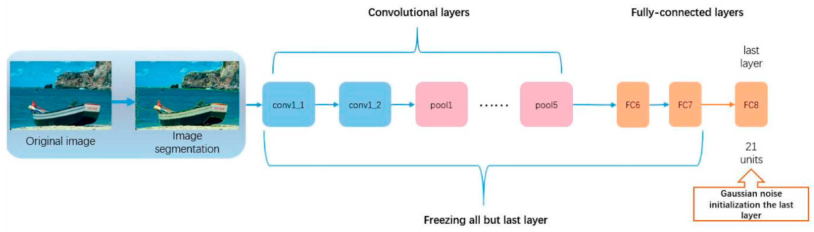
In this paper, image-level label semantic segmentation is used because there are many CNN-based network models, including VGGNet [26], GoogleNet [40], and ResNet [41]. Also, to reduce the computational resources in the experiment, we chose the VGG16 layer network model as shown in Figure 6 and converted the fully connected layer in the architecture into a convolutional layer. In the model, the more the layer is activated, the simpler the image is, so the network parameters of conv1-FC7 layer were first trained in ImageNet and remain unchanged during the process of transfer learning. We replaced the last layer with a layer of 20 object classes and a background class in the PASCAL VOC data set. The step size of this network is 32 s. However, instead of using the weight of the last layer from ImageNet, we chose to use random Gaussian noise to initialize the weight of the last layer; alternatively, we can also use the FC8 layer of VGG16 layer network.

Figure 6. This paper convolutional neural networks (CNN) model. Since our data set is small and similar to ImageNet, we used the method of freezing and training the last layer for transferring learning. The pre-trained network inner layer parameters (conv1-FC7) were transferred to the target classified by the PASCAL VOC object. For fine-scaled image edges and details, we initialized the last layer with Gaussian noise.

First, we used SLIC to segment the original image, and used Algorithm 1 to perform region merging on the generated super-pixels to obtain a set of candidate regions. Because they are aggregated by some super-pixels, they have a good region and edge properties. The trained FCN is then applied to the region-combined image and a pixel-wise prediction is generated. At the same time, using the ground truth annotation, we expect the prediction to overlap with the ground truth image. We define the overlapping objective function (6) as:

$${\epsilon }_o=\frac{1}{N}{\displaystyle {\displaystyle \sum }_S}\left(1-IoU\left(B,C\right)\right)\delta \left(sig{n}_B,sig{n}_C\right)$$

(6)

When the semantic label of the candidate region C is the same as the ground truth label of B, the function value is equal to 1, otherwise, it is equal to 0. The objective function is normalized. Also, to obtain an optimal solution, we minimize the objective function (7):

$$\underset{\theta ,\left\{sig{n}_C\right\}}{\min }{\displaystyle \sum }_i{\epsilon }_o$$

(7)

In order to bring the value of the objective function closer to 1, we apply the region merging algorithm to train the model. Furthermore, because the merged region of the superpixel can contain more edge details, we propose a greedy and iterative scheme to ensure the predicted results are closer to the ground truth. In the experiment, we also update the semantic label $sig{n}_C$ for all candidate regions. The semantic tag is updated by selecting the candidate region of the semantic tag and then iteratively merging the hyperpixel region of the neighborhood so that its cost ${\epsilon }_o$ is the smallest among all candidates. Finally, 20 object class semantic tags are assigned to the selected area, and other pixels are assigned as background tags.

In order to fix the semantic labels of all candidate regions, we repeatedly perform the region merge and predict the training steps. Then we determine a group of regions and predict another group region. With each iteration, we update the area markers for all images. Figure 7 shows the split picking pattern that is gradually updated during the training phase.

Figure 7. Semantic segmentation graph of different iteration times. The number of iterations is epoch #1, epoch #4, epoch #8, and epoch #10.

According to our proposed Algorithm 2, the final semantic segmentation result is obtained.

Algorithm 2. Superpixel merge semantic segmentation

1.  Construct the SLIC split graph.

2.  Build super pixel area merge map.   The parameters are as follows:   The superpixel region is set as $\mathrm{C}=\left\{C_1,C_2,\cdots ,C_k\right\}$.   Also, the semantic label $sig{n}_C\in \left\{0,1,\cdots ,20\right\}$ in the area $C_i$ is initialized to 0, and 0 is the background label.

3.  Iteratively generate semantic segmentation by using region merging algorithm. Loop: for epoch = 1:Epoch 3.1 Use the FCN to generate a rough prediction map and update the semantic label $sig{n}_C$ belonging to the prediction area $C_i$ from formula (1). 3.2 Calculate the overlap value between the obtained graph and the ground truth value (function (6)) and minimize the objective function (7) to determine whether it is close to 1. 3.3 If it is close to 1, end the iteration and go to step 4. Otherwise update the parameters of the merged area. 3.4 Calculate a plurality of adjacent regions $C_i$, and generate a neighborhood set $\mathrm{neighbours}=\left\{\left(C_i,C_{n1}\right),\left(C_i,C_{n2}\right),\cdots ,\left(C_i,C_{nk}\right)\right\}$, and perform the super pixel region merging algorithm. Go back to step 3.1.

4.  Output semantic result graph.

4. Experiment Analysis

Our test bed consists of Xeon E5-2609 v3 CPU, 32G RAM, hard disk 3T, Windows10 x64 operating system, and Ubuntu 16.04 LTS operating system with Matlab R2016a platform, and Caffe deep learning framework.

4.1. Data Set

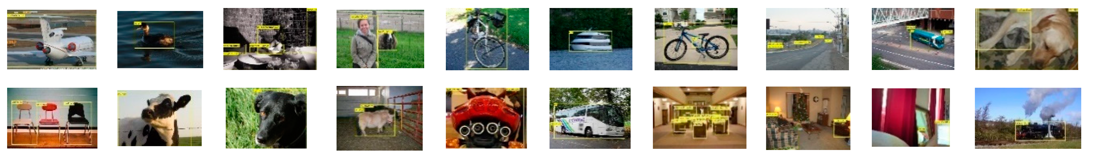
We performed image semantic segmentation on the PASCAL VOC 2012 dataset to evaluate our approach. Figure 8 shows that the data set contains 20 object class tags and a single background class tag.

Figure 8. Twenty categories.

A total of 10,582 training images and a VOC2012 validation set containing a total of 335 images remained unchanged in this work.

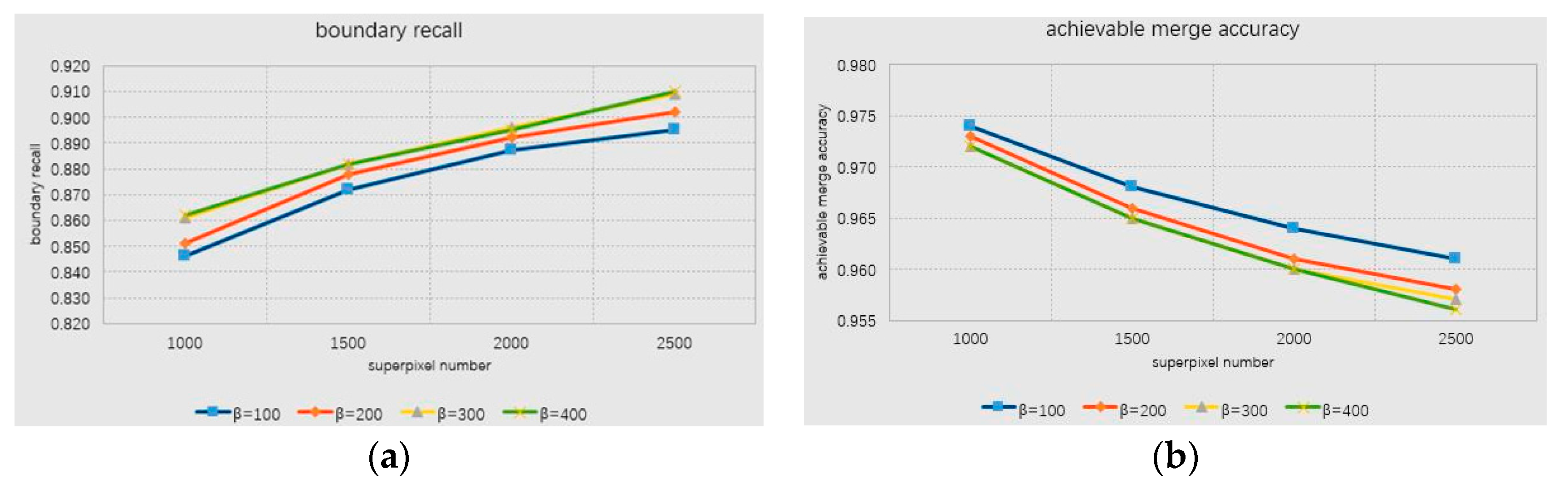
4.2. Parameter Sensitivity of Regional Combination

In order to assess the performance of the superpixel region merging algorithm, we studied the effects of different parameters, for instance, the weight size, the number of super-pixels, and the amount of regions after fusion on the segmentation results. We tested on the VOC 2012 dataset, the standard metric [42] is the boundary recall (BR) and the achievable segmentation accuracy (ASA). The boundary recall measures the percentage of the natural boundaries recovered by the superpixel boundaries while the achievable segmentation accuracy gives the highest accuracy achievable for object segmentation that utilizes super-pixels as units [42].

Figure 9 reveals the performance changes for different shape parameter α. In respect of BR, the monotonic value of BR reduces. When α ≤ 0.2, there is only a slight change. In the case of BR and ASA, the curve trend is nearly similar and both decreasing as the amount of pixels increases, and the value of α increases as well. In order to make the number of super-pixels as consistent as possible and avoid significant reduction of the segmentation precision, we set 0.3 ≤ α ≤ 0.9. Also, the number of super pixels is controlled at 600–1500.

Figure 9. Different α segmentation performances, (a) represents the performance curve of different α values of boundary recall, (b) represents the performance curve of different α values of achievable merge accuracy. We set the function $f\left(x\right)=-x\log \left(x\right),\gamma =0.3$.

Similarly, we studied the effect of regional compaction on the regional fusion in the range of 0.2–1.0. The results obtained are very small and the curve of BR and ASA almost overlaps. In addition, the influence of the number of combined regions, $\gamma$ on the quality of segmentation, is also tested. Figure 10 shows the performance changes in the case of different parameters.

Figure 10. Different $\gamma$ segmentation performances, (a) represents the performance curve of different $\gamma$ values of boundary recall, (b) represents the performance of different $\gamma$ values of achievable merge accuracy. We set the function $f\left(x\right)=-x\log \left(x\right),\alpha =0.3$.

In summary, we select the parameters in the iterative process of regional fusion: shape parameter is α, and number of combined regions ($\gamma$). We have the greatest impact on the combined results. Therefore, the interval for setting α is 0.3–0.9, and the interval for $\gamma$ is 10–100. In this interval, the speed of the region merging process can be made more efficient and accurate.

4.3. Index

Semantic segmentation performance is based on previous work [43]. We used the standard intersection over union (IoU) metric, also known as the Jaccard Index [44], to evaluate our results. It is defined as the percentage of pixels in each category that is marked or classified as predicted pixels in the total pixel of the category.

4.4. Qualitative Analysis

According to our proposed method, Figure 11 shows the comparison between the proposed RMNN method and constrained convolutional neural networks (CCNN) with size as a constraint [35] on the VOC 2012 dataset.

Figure 11. The semantic segmentation obtained by combining region merging and CNN. (a) The original images. (b) Superpixel region merge results. (c) Constrained Convolutional Neural Networks (CCNN). (d) RMNN. (e) The ground truth. See also Table 1.

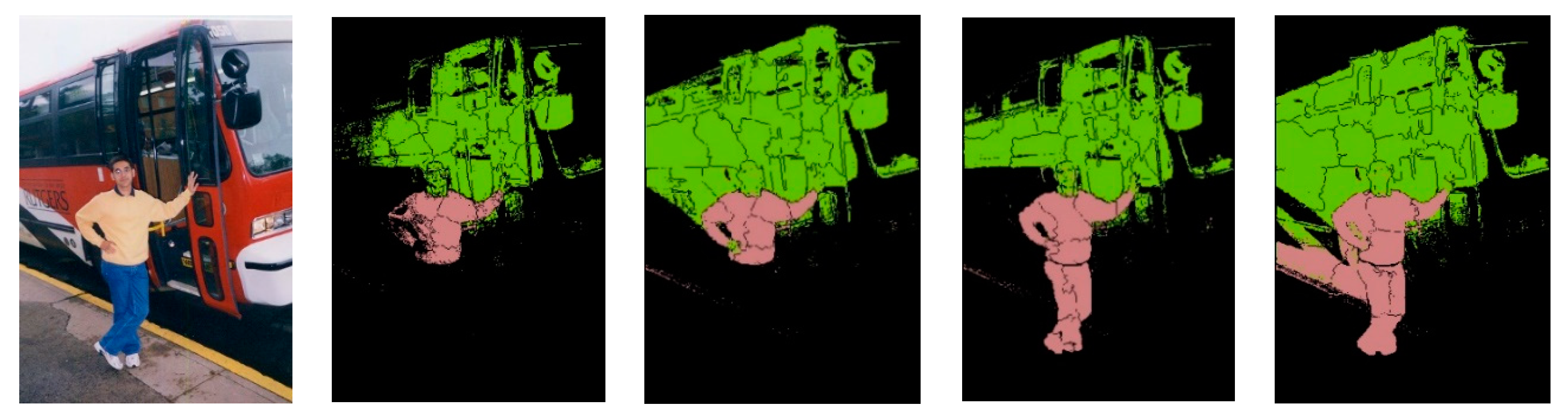
As shown in Figure 11, the weakly-supervised semantic segmentation maintains the basic overall contour of the target due to the excellent performance of the superpixel segmentation and region merging algorithm. At the same time, it is also reflected in the details of the target. The general image-level semantic segmentation can only guarantee the outline of the target but cannot identify some details of the target. However, our algorithm can improve the recognition of certain details in the target while maintaining the basic shape. In (c), (d), we can observe that the proposed algorithm is superior to the CCNN method, and our algorithm can achieve better accuracy on the contour of the target. Although our algorithm is slightly inferior in the second set of figures, the overall outline of the target is still identified. In summary, our approach is superior to some weakly-supervised semantic segmentation such as CCNN, especially in the ability to maintain the contour of the target. Also due to the nature of the regional merger, it is difficult to generalize the shape of some small objects. For example, the fifth image in Figure 11 does not identify the distant train, so there is still room for improvement in this respect. We have left this for future work.

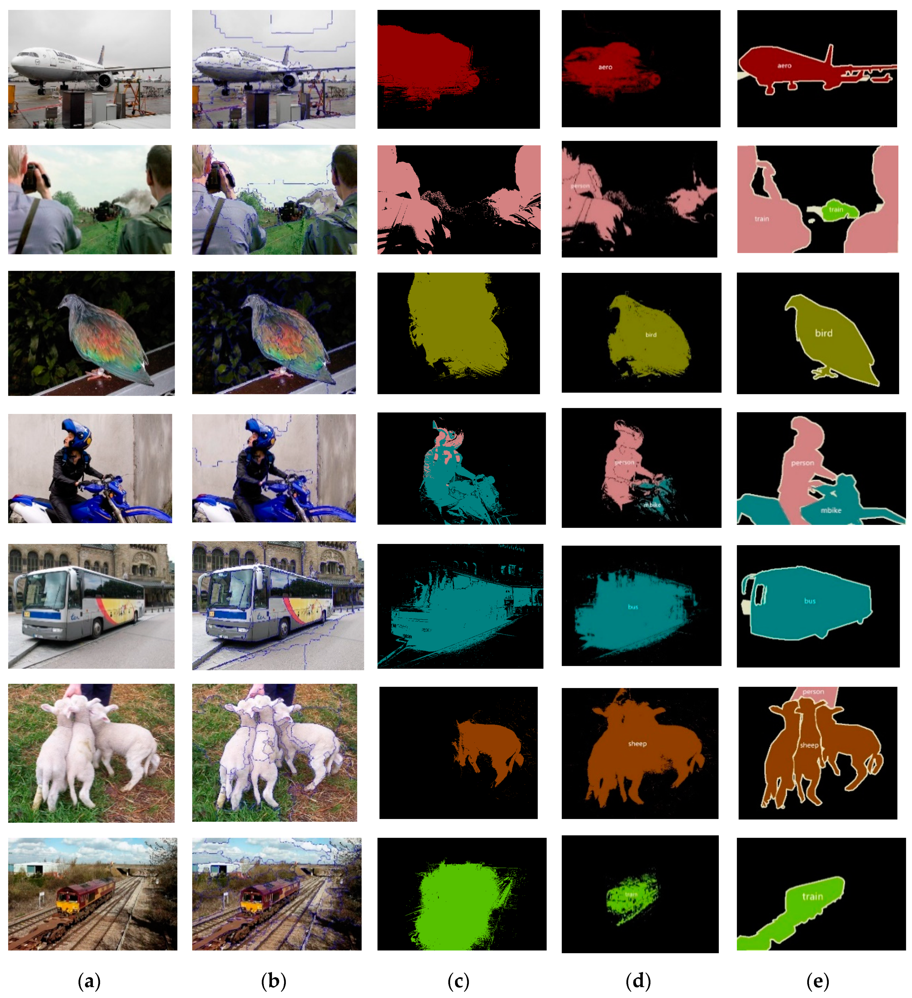
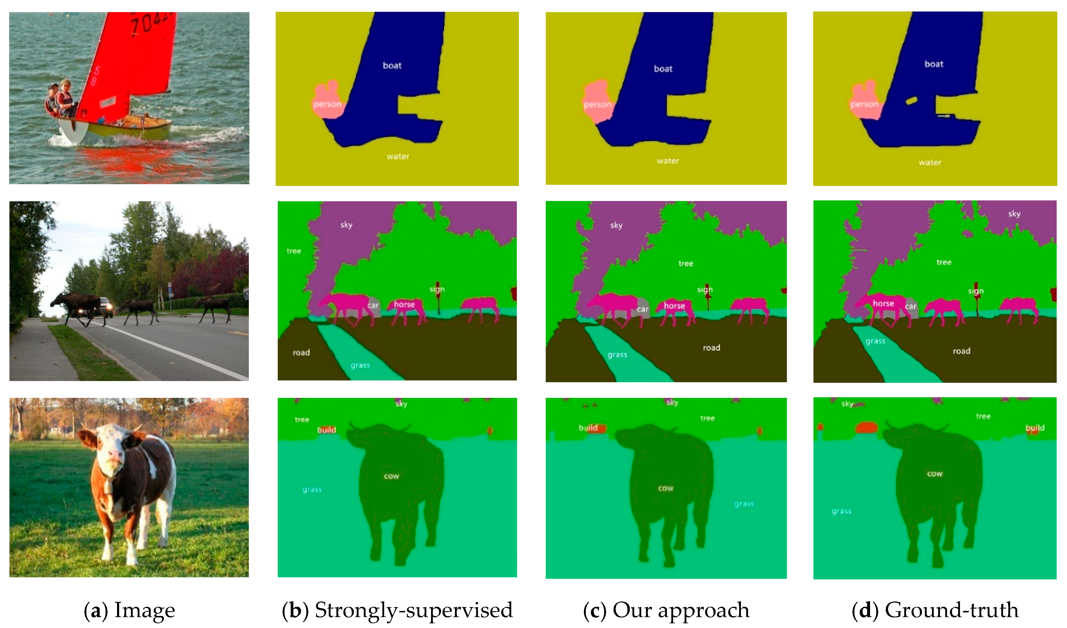
We further performed experiments on the labeled PASCAL-CONTEXT dataset [45]. The dataset provides semantic labels for all targets, including grass, sky, and water. The model was trained on images of 5K resolution (fine notes only). We replaced 21 categories in the original framework with 60 categories, and we used IoU to assess accuracy. In addition, CRF was used as a post-processing step in the framework because the semantic tag contains the entire scene. Some examples of PASCAL-CONTEXT are shown in Figure 12.

Figure 12. Results on PASCAL-CONTEXT dataset.

Our results show that the strongly-supervised mean IoU (mIoU) on the PASCAL-CONTEXT dataset was 48.1%, and the score based on the proposed super-pixel weak supervision method was 45.9%. Although our score was lower than the strong supervision, it was 1.3% higher than the PASCAL VOC score. It shows that more tag comments can improve the precision of semantic segmentation.

4.5. Quantitative Analysis

In our experiments, we used some indicators (IoU, mIoU, PA) to evaluate our algorithm, and we observed that our method achieves better performance in weakly-supervised segmentation. First, using the IoU briefly discussed in Section 4.3, Table 1 compares some of the contemporary weak segmentation methods. Pinheiro and Collobert [34] proposed several semantic segmentations based on the multi-instance learning (MIL) framework. The model pays more attention to the rearrangement of pixels in image classification; hence, the algorithm is sensitive to the initialization of images and improves the accuracy of distinguishing correct pixels by using a small number of smooth priors. The initial step of the RMNN is to perform superpixel constraints, and constrained optimization relies on superpixel combining during iterative training. The initial step of RMNN is to perform super-pixel segmentation. For each image I, we can obtain a set of super-pixel tags $sing{n}_{C_0}$. Our superpixel merging can encourage multiple pixels to add constraints by merging to get the outline of the target. While this approach encourages certain pixels to use a specific label, it is usually insufficient to correctly label all the pixels. We constrain the target by super-pixel merging to form a super-pixel block and mark the target foreground as much as possible. This distinguishes the foreground and background labels, iteratively synthesizes larger areas, and ensures that the final mark is as close as possible to the outline of the target. The EM-Adapt method [12] proposes an expectation maximization (EM) method under weakly-supervised and semi-supervised conditions, and it focuses on the most unique part of the object (such as a human face) rather than capturing the entire object (such as the human body). On the contrary, our method focuses on the overall contour of the target, but it is less sensitive to the recognition of some small objects. We compared the IoU values obtained from applying the weakly-supervised semantic segmentation categories on PASCAL VOC 2012 dataset, and we can conclude that the RMNN has significant improvement in overall performance over other methods.

Table 1. Comparison of several weakly-supervised semantic segmentation methods on PASCAL VOC 2012 data set, the IoU score for each level of the VOC data set is presented and the best performance is highlighted in bold.

Category	EM-Adapt [12]	MIL-Base [34]	CCNN with Size (CRF Tuned) [35]	Proposed (RMNN)
bgnd	66.8	38.1	65.8	67.1
aero	28.9	11.1	42.3	36.3
bike	17.2	18.4	24.5	28.6
bird	29.7	11.3	56.0	54.4
boat	21.9	05.4	30.6	29.6
bottle	29.6	06.1	35.0	36.4
bus	47.3	25.3	58.8	51.3
car	46.7	23.5	52.7	53.1
cat	47.8	26.4	54.8	50.3
chair	13.9	04.8	14.6	26.2
cow	38.8	23.6	48.4	50.4
table	21.3	08.7	34.2	37.6
dog	34.6	30.8	52.7	58.1
horse	45.6	22.1	46.9	48.6
mbike	39.3	26.5	61.1	56.6
person	36.5	22.3	44.8	46.3
plant	25.3	13.6	37.4	40.2
sheep	37.4	30.2	48.8	45.9
sofa	24.4	08.4	30.6	32.6
train	32.4	19.9	47.7	51.2
tv	32.8	15.2	41.7	36.3

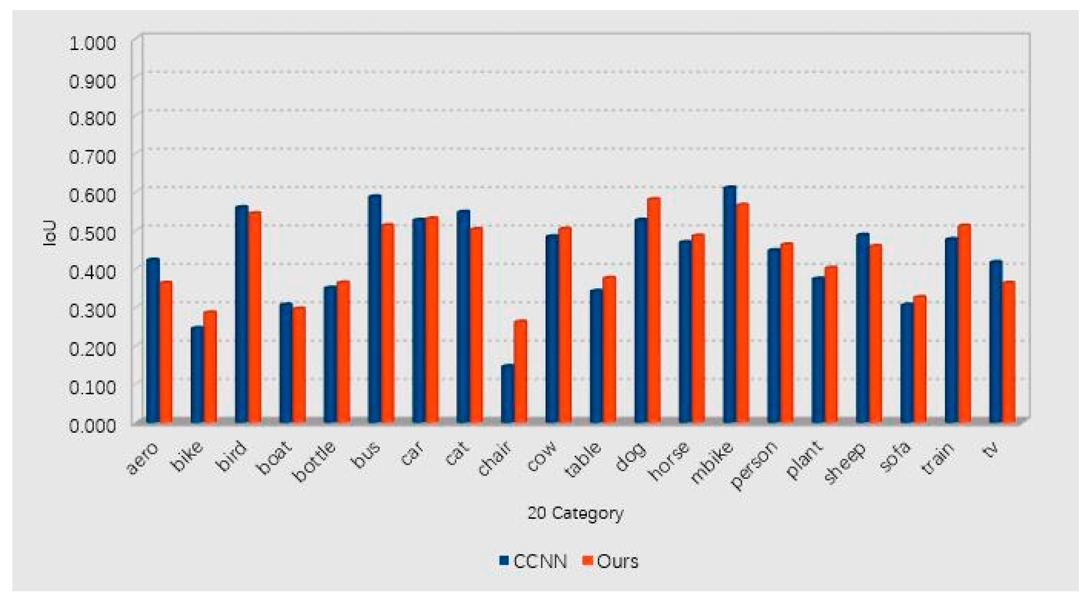
The CCNN [35] method proposes a series of constraints for semantic segmentation, either using a single constraint or a superposition of multiple constraints. This method can be used in several existing frameworks, we chose size as a constraint to compare with our method. The x-coordinate values are the 20 categories of PASCAL VOC 2012. Figure 13, drawn from the data in Table 1, shows the IoU comparison between CCNN and the proposed RMNN.

Figure 13. RMNN and CCNN segmentation accuracy.

Secondly, we use the average or mean intersection over union (mIoU) (Equation (8)) and pixel accuracy (PA) [43] in Table 2. PA is the ratio of the number of correctly classified pixels to the total number of pixels. This is a standard indicator used for subdivision purposes to calculate the ratio between ground truth and predicted results. mIoU is derived by calculating the average IoU. Suppose the total amount of classes is $\left(n+1\right)$ and $p_{ij}$ is the amount of pixels of class i inferred to class j. $p_{ii}$ represents the number of true positives, while $p_{ij}$ and $p_{ji}$ are usually interpreted as false positives and false negatives [31].

Table 2. The mean intersection over union (mIoU) and pixel accuracy (PA) scores of the four methods.

Metric	mIoU	PA
EM-Adapt	34.2	56.8
MIL-Base	18.7	48.6
CCNN	44.3	63.2
RMNN	44.6	62.1

$$\{\begin{array}{c}mIoU=\frac{1}{n+1}\times {\displaystyle \sum }_{n}Io{U}_n\\ IoU=\frac{p_{ii}}{{{\displaystyle \sum }}_{j=0}^n{p}_{ij}+{{\displaystyle \sum }}_{j=0}^n{p}_{ji}-p_{ii}}\end{array}$$

(8)

During the experiment, we only considered image-level labels and used superpixel region merging to improve the results of weakly-supervised semantic segmentation. This saves time on commenting the target and does not require the user’s input. Table 3 shows the comparison of our method with the fully supervised method for mIoU and PA scores.

Table 3. We compare the fraction of pixel level semantically segmented mIoU and pixel accuracy (PA).

Category	DeepLab-CRF	Fcn-8s	Ours
mIoU	64.6	61.1	44.6
PA	76.8	81.4	62.1

Weakly-supervised semantic segmentation performs poorly when compared with the more complex systems that use more segmentation constraints in terms of the pixel accuracy and mIoU. We believe that the key to this difference in performance is pixel-level segmentation information. Although RMNN has a good effect, it lacks the important factor of object characteristics, hence, the gap with the pixel level is huge. In future research, we plan to enhance the image-level competitive advantage by extracting the color, texture, and other features of the image.

5. Conclusions and Future Work

This paper proposes a weakly-supervised semantic segmentation method using superpixel aggregation as an annotation. The method combines super-pixels with similar features using superpixel color and texture features. This forms an annotation of the target object to achieve the design objective. Specifically, we split the image into super-pixels and into the detailed features of each superpixel. We experimented with the pros and cons of the three merge criteria and determined that the third criterion to merge the target’s super-pixels would work better. Since the data set in the experiment is PASCAL VOC 2012, there may be some problems if the network trained on ImageNet is directly applied to the Pascal VOC. Because the source data set and the target data set may be very different, this paper uses migration. The way we learn, we can use the small data set PASCAL VOC to fine tune the network (trained on ImageNet) so that the network can be used for small data sets. Through the training flow diagram of this paper, we predict the semantics of the super-pixels of the merged region and use our basic fact value comparison to feed the intermediate results back to the optimization function, and optimize the function iteration to the final optimal value. The experimental results show that the proposed RMNN approach can achieve more accurate segmentation results compared to state-of-the-art weakly-supervised segmentation systems. The score reached 44.6%.

Although our algorithm has a good mIoU score, it can still be improved. One limitation of the proposed approach is that it is not optimal for small objects; in future work, the distance between the elements covering the convolution kernel of the network model needs to be increased, and the convolution is no longer performed in the continuous space. We also plan to use dilated convolution to reduce the loss of more small features. A long-term goal is to integrate the proposed method to some popular big data systems (e.g., Spark) as image processing is considered as one of the most data-intensive workloads in many scientific domains [46].