Article

Two-Level Fault Diagnosis of SF6 Electrical Equipment Based on Big Data Analysis

1
College of Internet of Things Engineering, HoHai University, Changzhou 213022, China
2
Electrical Engineering institute, Guangxi University, Nos.100, East University Road, Nanning 530004, China
*
Author to whom correspondence should be addressed.
Big Data Cogn. Comput. 2019, 3(1), 4; https://doi.org/10.3390/bdcc3010004
Submission received: 9 November 2018 / Revised: 19 December 2018 / Accepted: 21 December 2018 / Published: 3 January 2019

Abstract

:
With the increase of the operating time of sulphur hexafluoride (SF6) electrical equipment, the different degrees of discharge may occur inside the equipment. It makes the insulation performance of the equipment decline and will cause serious damage to the equipment. Therefore, it is of practical significance to diagnose fault and assess state for SF6 electrical equipment. In recent years, the frequency of monitoring data acquisition for SF6 electrical equipment has been continuously improved and the scope of collection has been continuously expanded, which makes massive data accumulated in the substation database. In order to quickly process massive SF6 electrical equipment condition monitoring data, we built a two-level fault diagnosis model for SF6 electrical equipment on the Hadoop platform. And we use the MapReduce framework to achieve the parallelization of the fault diagnosis algorithm, which further improves the speed of fault diagnosis for SF6 electrical equipment.

1. Introduction

SF6 electrical equipment refers to electrical equipment that uses sulphur hexafluoride (SF6) as insulation or arc extinguishing. SF6 electrical equipment has the advantages of small size, small maintenance, long life and good insulation. With the extensive popularization of intelligent substation, there are more and more power equipment [1]. The traditional oil-filled equipment is being replaced gradually by SF6 electrical equipment which have unique advantages and account for an increasing proportion of new equipment. With the increasing number of SF6 electrical equipment, the reliability requirements have also increased [2]. The internal discharge of SF6 electrical equipment leads to the decomposition of internal SF6 gas molecules. The chemical properties of its derivatives are very active. The derivatives can corrode the equipment, which can easily cause a decline in the insulation performance and cause serious damage to the safe and stable operation of the equipment [3,4].
In the literature [5], the phenomenon that the decision tree model or the radial basis function (RBF) neural network model is not used when the diagnosis is not high is firstly described. Then the RBF neural network and the decision tree model are used to diagnose the SF6 electrical equipment. This method requires two diagnostics for all data, which will take a lot of time.
The continuous creation of data has posed new research challenges due to its complexity, diversity and volume. Consequently, Big Data has increasingly become a fully recognized scientific field [6]. Now big data analytics are increasingly being used to solve real-world problems in life [7]. And the cloud platform provides an open architecture for big data analytics, which can improve the utilization of data resources [8].
The arrival of the era of big data is accompanied by massive data, which makes the screening of valuable information a core step in the widespread application of big data. Hadoop is an open source distributed computing platform, its distributed file system HDFS and distributed computing framework MapReduce solved the problem of data storage and programming [9]. Hadoop’s ability to store and process data in bits is trusted. The backup mechanism is used in HDFS to maintain multiple copies of data. The task monitoring mechanism is used in MapReduce. Hadoop is able to dynamically move data between nodes and ensure the dynamic balance of each node, so processing is very fast [10].
MapReduce is a programming model and related implementation for processing and generating large data sets that are suitable for a wide variety of practical tasks [11]. MapReduce advantages over parallel databases include storage-system independence and fine-grain fault tolerance for large jobs [12]. At the same time, MapReduce can realize parallel processing of data and greatly improve the processing efficiency of monitoring data of SF6 electrical equipment [13].
In order to solve the above problems, the two-level fault diagnosis model of SF6 electrical equipment based on the content of SF6 gas derivative as the input for the monitoring data of SF6 electrical equipment was proposed in this paper. The first level fault diagnosis model is first used to determine whether the data is fault data. If yes, it enters the second level fault diagnosis model to identify the specific fault category. If not, the judgment is no longer performed, thereby improving the diagnostic efficiency. In order to quickly realize the fault diagnosis of SF6 electrical equipment for the massive SF6 electrical equipment condition monitoring data, this paper implements the fault diagnosis of SF6 electrical equipment on Hadoop platform and realizes the parallelization of SF6 electrical equipment fault diagnosis algorithm.

2. The Two-Level Fault Diagnosis Model for SF6 Electrical Equipment

2.1. Data Acquisition of SF6 Electrical Equipment

The two-level fault diagnosis model diagnoses the equipment by the content of SF6 gas derivatives. Therefore, it is necessary to select SF6 gas derivatives as the characteristic attributes first. When partial discharge occurs in SF6 electrical equipment, SF6 gas decomposes to produce a variety of derivatives. The formation mechanism of the derivatives is very complex, and mainly includes two processes. First, the SF6 gas decomposes to generate low fluorides, and then these low fluorides react with impurities, electrode materials, and insulating materials to generate other more stable derivatives. Derivatives derived from different discharge energies are also different. According to the magnitude of the released energy, discharge can be divided into three forms: arc, spark and corona discharge. Some references [14,15,16] mention that there is a large amount of SOF2 and a small amount of SO2F2 generated under arc discharge. The main derivative of spark discharge is also SOF2, in which the content of the derivative content is: SOF2 > SOF4 > SO2F2 > SO2 > S2F10/S2OF10 [17]. During corona discharge, SOF2 is still the most abundant derivative, and the contents of SO2F2, S2OF10, and S2F10 are higher than those of the other two discharges. Therefore, SOF2, SOF4, SO2F2, SO2, S2OF10, and S2F10 were selected as the characteristic attribute of the algorithm [18]. And the types of faults in SF6 electrical equipment can be divided into three main types: arc, spark and corona discharge.
Infrared spectroscopy is a method for the quantitative and qualitative analysis of various infrared light absorbing compounds. The composition is analyzed by the difference in the absorption of infrared radiation by the substance. One of the great advantages of infrared spectroscopy is that virtually any sample may be studied in any state [19]. Infrared spectroscopy can be used to analyze the composition of SF6 gas in electrical equipment to determine the state of the equipment [20]. Infrared spectroscopy can be used to detect large quantities of material at a lower cost [21]. Therefore, we can install an infrared spectrum analyzer for gas composition analysis and data acquisition in SF6 electrical equipment.

2.2. Construction of two-level fault diagnosis model

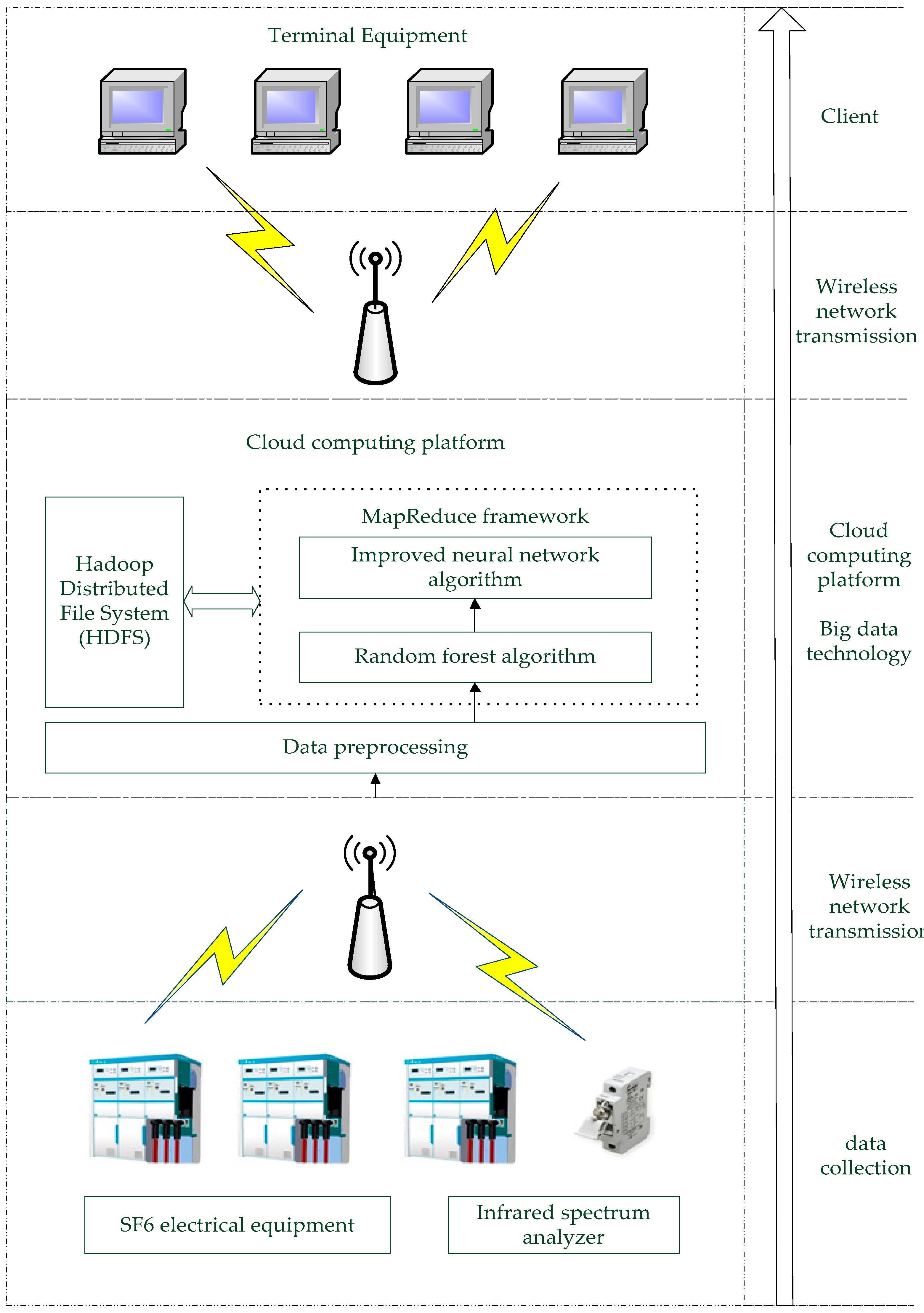
The first level model is constructed using a random forest algorithm. The random forest model is used to filter out the fault data. Because it is only used to determine whether the equipment is faulty, the depth of the decision tree constructed in the forest is low, which can reduce the diagnosis time. The second level model is built by the neural network algorithm. The input was fault data filtered by a random forest model. The second-level model can not only diagnose the known types of faults, but also identify the new fault types through communicating with experts. And by updating the structure and weight of the neural network model, the model is continuously improved. Figure 1 is a block diagram of the SF6 electrical equipment fault diagnosis system.
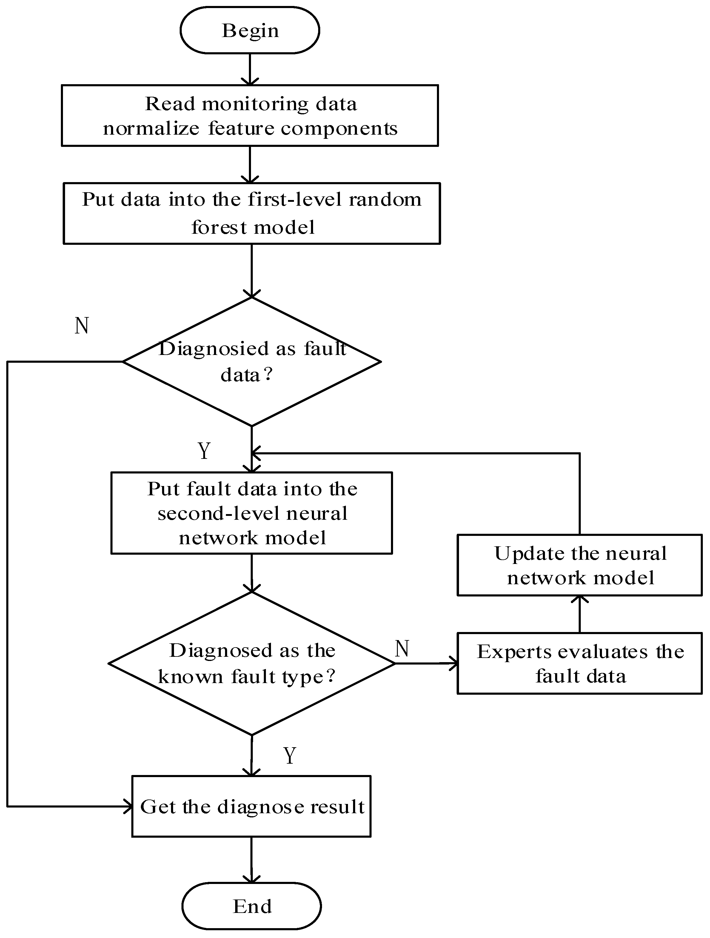
The fault diagnosis process of SF6 electrical equipment is shown in Figure 2, and the main steps are follows.
(1)
Reading monitoring data, extract feature components and category components, then normalizing the feature components.
(2)
Putting the normalized data into the first-level random forest model. If the data is diagnosed as normal data, then output the result directly. Otherwise, go to step 3.
(3)
Putting the data that diagnosed as fault data in step 2 into the second-level neural network model. If the fault type of the equipment has been trained, then output the diagnosis result directly. Otherwise, go to step 4.
(4)
The fault type that cannot be correctly identified in step 3 is submitted to the experts for diagnosis to determine the type. Then the neural network is retrained to update the structure and weights of network so that it can be continuously improved.
The specific algorithm can refer to our paper: The two-level fault diagnosis model of SF6 electrical equipment [18].
Figure 3 is the architecture diagram of the secondary fault diagnosis system for SF6 electrical equipment.

3. Monitoring Data Preprocessing

The fault diagnosis of SF6 electrical equipment is one of the methods to verify the operation status of the equipment, but the detection model of the equipment is mostly based on an ideal data set [22]. In the actual collection process, data redundancy, data loss, and data inconsistency will inevitably occur due to issues such as collection equipment, external environmental disturbances, and human’s misoperation. This will eventually affect later data mining. Therefore, before the fault diagnosis of SF6 electrical equipment, this section fills in the missing values in the monitoring data to implement data pre-processing, and then implements the algorithm.
There are currently few data preprocessing studies on SF6 gas derivative monitoring data. In this section, the SF6 gas derivative content data is used as the processing object. Through the analysis of the data, it is found that there may be three cases of the missing monitoring data. A single approach cannot be fully applied to all situations. Therefore, the data missing values are classified, and different processing methods are adopted for each case.
There are three possible missing values for SF6 gas derivative content monitoring data. These three conditions are described as follows.
(1)
The missing value is in the same range as the monitoring value recorded before and after it. There are two cases. Case 1: Monitoring data including missing values over a period of time is within normal limits. Case 2: Due to equipment failure, the monitored data including missing values over a period of time is in an abnormal range.
(2)
The missing value is not in the same range as the monitoring value recorded before and after it. There are also two cases. Case 1: The device just fails and the SF6 gas derivative content rises from the normal range to the abnormal range. Case 2: The equipment was repaired and the content of SF6 gas derivatives dropped from the abnormal range to the normal range.
(3)
The monitoring values are lost over a period of time.
For the above three cases, the process is as follows.
(1) The weighted interpolation method is used to deal with the case where the first type of data is missing, that is, the weighting factor is introduced for the mean interpolation method.
The basic mean interpolation method takes the arithmetic mean of the n numbers before and after the missing value as a substitute value, as shown in Equation (1).
H t = 1 2 n ( i = 1 n H t i + i = 1 n H t + i )
The weighting factor is introduced for the mean interpolation method, as shown in Equation (2), wherein the record closer to the missing value time has a larger weight.
H t = i = 1 n w t i H t i + i = 1 n w t + i H t + i
where w is the weight, the closer to the missing value, the greater the weight of the record.
There are six kinds of SF6 gas derivatives selected in this paper, and SOF2 is used as an example for pretreatment. In order to verify the validity of the algorithm, some SOF2 historical data was read from the database and created some missing cases. In the experiment, four monitoring values were chosen to estimate missing values. When SF6 electrical equipment is in normal condition, its SOF2 content does not exceed 10 μ L / L .
In this section, multiple sets of experiments were performed for each type of data loss. For reasons of space, only a part of the content was selected as the result.
Experiment 1: The historical data of SOF2 are within the normal range. The experimental data is shown in Table 1. The numerical values of the serial numbers 3, 4, and 5 are removed in turn, and the interpolation results of SOF2 are shown in Table 2.
Using the weighted interpolation method to calculate the missing values as follow:
H 3 = w 1 H 1 + w 2 H 2 + w 3 H 4 + w 4 H 5 = 6.53
where w 1 = w 4 = 0.2 , w 2 = w 3 = 0.3 .
According to Table 2, the average error of the mean interpolation method is 5.3%, and the average error of the weighted interpolation method is 4.8%. In this case, the weighted interpolation method works well.
Experiment 2: The historical data of SOF2 are within the abnormal range. The experimental data are shown in Table 3. The numerical values of the Nos. 3, 4, and 5 are removed in turn, and the interpolation results of SOF2 are shown in Table 4.
According to Table 4, the average error of the mean interpolation method is 4.12%, and the average error of the weighted interpolation method is 3.86%. The weighted interpolation method works well.
(2) Reading the SOF2 monitoring data from the database for a period of time. The missing value is not in the same range as the monitoring value recorded before and after it.
Experiment 3: When the content of the previous monitoring data of SOF2 missing value is within 10 μ L / L , and the content of the latter monitoring data is greater than 10 μ L / L , it indicates that the content of SOF2 fluctuates from the normal range to the abnormal range. The experimental data is shown in Table 5. If the experiment is continued using the weighted interpolation method and the mean interpolation method, the numerical values of the serial numbers 3 and 4 are sequentially removed, and the experimental results are shown in Table 6.
It can be seen from Table 6 that although the error of the interpolation can be reduced by adjusting the weight, it is necessary to find a suitable weight. For sequence number 3, the method of linear interpolation is not suitable.
(3) When the SOF2 monitoring data is read from the database for a period of time, there is a continuous lack of data, and the linear interpolation method cannot be used at this time.
Considering case 2 and case 3, this paper uses the gray correlation degree to interpolate the data. The SF6 gas derivative content data complementing method based on gray correlation is to perform gray scale processing on other component data except the missing value attribute, and to find the closest set of data with the missing value tuple by calculating the correlation degree to make up the complement treatment. The main process is shown in Figure 4.
The specific steps are follows:
Step 1: Determining the main sequence and subsequence.
A tuple containing missing values is taken as the main sequence. A tuple, in the historical record, with at least one attribute value that is not within the normal range of the safety work is taken as a subsequence. Mark them as X 1 X m and m = 5000 .
Step 2: The matrix formed by the main sequence and subsequences is standardized to obtain a normalized matrix X.
Step 3: Calculate correlation coefficient.
The formula for calculating the correlation coefficient r e l ( i ) of X i for X 0 is:
r e l ( i ) = min A b s V a l u e ( i ) + d e f max A b s V a l u e ( i ) a b s V a l u e ( i ) + d e f C max A b s V a l u e ( i )
a b s V a l u e ( i ) = a b s ( X i X 0 )
where a b s V a l u e ( i ) is the absolute difference sequence of X i and X 0 , min A b s V a l u e ( i ) and max A b s V a l u e ( i ) are the minimum and maximum of a b s V a l u e ( i ) , d e f C ( 0 , 1 ) is the resolution coefficient and d e f C = 0.5 .
Step 4: Calculate relevance.
The formula for calculating relevance p ( i ) of X i for X 0 is:
p ( i ) = r e l ( i ) * w
where w is the weight of each SF6 gas derivate. There are six kinds of derivatives, so the w is set to 1/6.
Step 5: Interpolated missing values.
Sorting the relevance obtained above, and extracting the first 10 sets of tuples those relevance are greater than 0.9 are taken to interpolate the missing values. If less than 10 sets, all the tuples satisfying the condition will be taken. The formula for interpolating missing values X 0 j is:
X 0 j = 1 n i = 1 n X i j
where j is the column of the missing value in the tuple, n is the number of tuples taken.
Experiment 3 was re-examined using the gray correlation degree. The experimental results are shown in Table 7.
From Table 7, it can be seen that the interpolated values for Nos. 3 and 4 are 8.51 and 13.32, the errors are 0.01 and 0.033 respectively. Therefore, the use of gray correlation can effectively solve the problem of missing data mutations.
The method of grey correlation is to find the closest tuples in the previous record to interpolate missing data. Therefore, when this method is used, there is no case of continuous lack of data.
After pre-processing the monitoring data of the SF6 electrical equipment, a two-level fault diagnosis model of the SF6 electrical equipment can be constructed. First, we train the model on the Hadoop platform. Second, we implemented parallelization of diagnostic algorithms on the Hadoop platform.

4. Implementation of the Two-Level Fault Diagnosis of SF6 Electrical Equipment Based on Hadoop

Hadoop is an open source distributed computing platform. Its distributed file system (HDFS) and distributed computing framework (MapReduce) solve the data storage and programming problems, respectively. Therefore, we implemented the parallelization of the above fault diagnosis algorithm on the Hadoop platform, which improved the processing speed of massive monitoring data and accelerated the diagnostic rate of SF6 electrical equipment.

4.1. Implementation of Random Forest Algorithm Based on MapReduce

After preprocessing the SF6 electrical equipment monitoring data, a two-level fault diagnosis model of the SF6 electrical equipment can be constructed on the Hadoop platform, and the parallel algorithm of the diagnostic algorithm can be realized through the Hadoop platform.
In the process of establishing a random forest, each decision tree is created in a serialized manner. Only when the current decision tree is generated will the next tree be created. Decision trees are independent of each other, and there is no need to rely on other trees when creating a decision tree, so parallelization can be achieved.
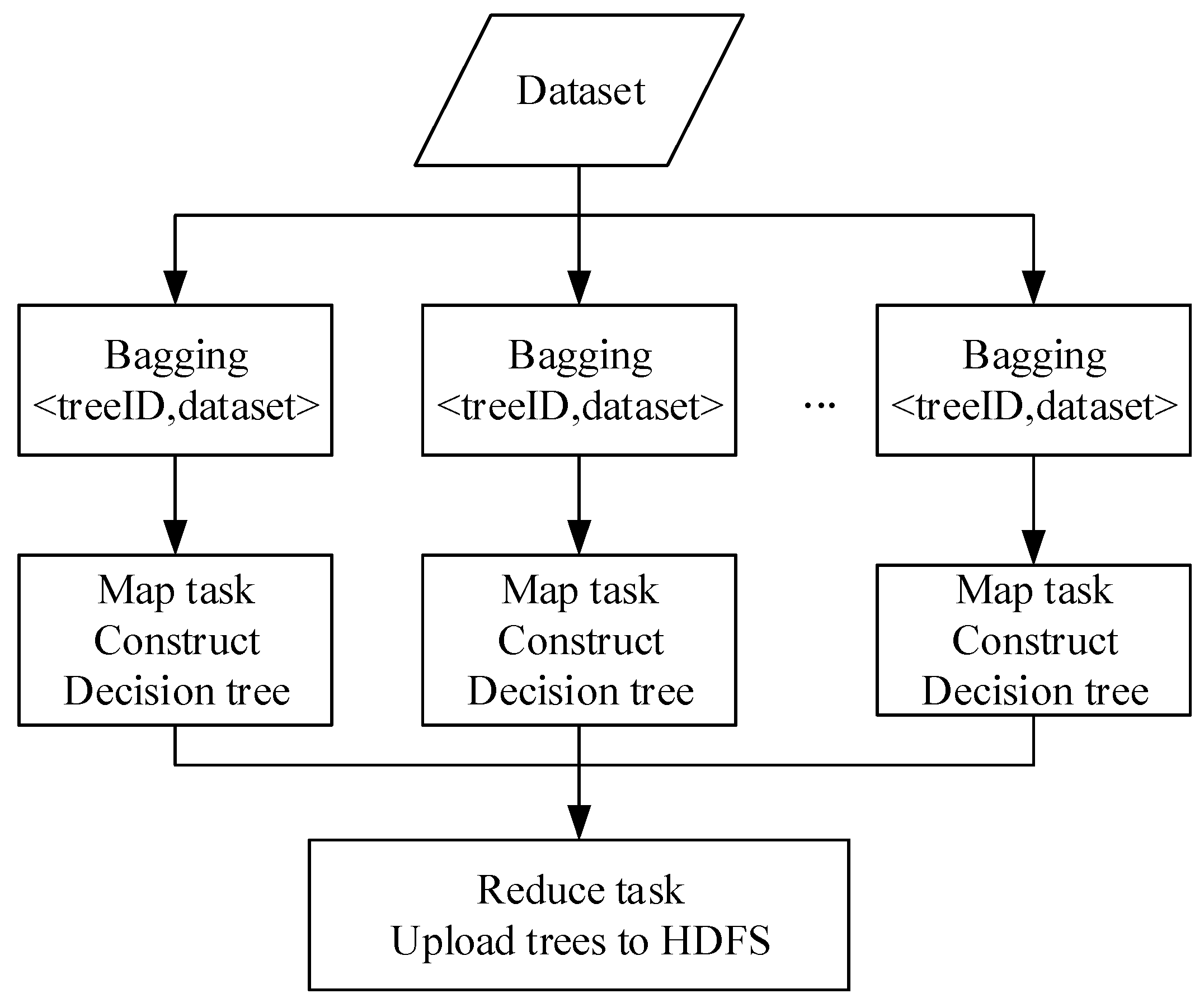
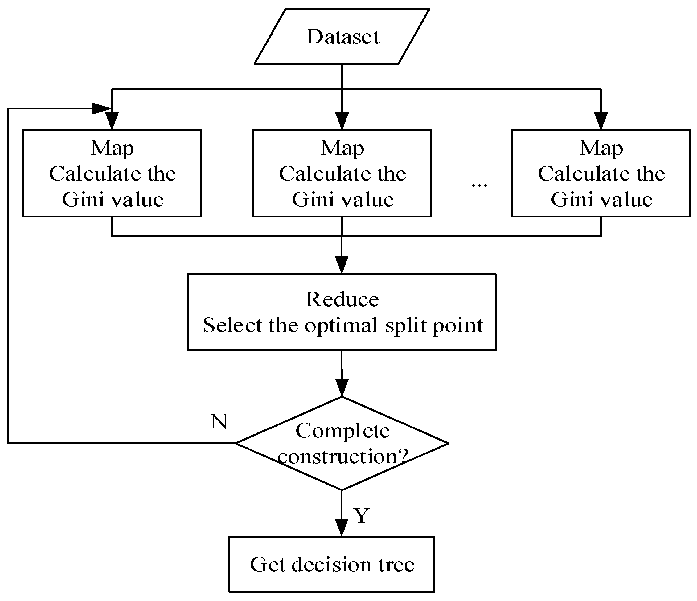
Using the MapReduce framework to achieve the parallelization of the random forest algorithm mainly has two stages: Map and Reduce. Each Map task establishes a decision tree, and finally uploads them to HDFS in the Reduce task to form a forest. The parallel forest construction process of random forest is shown in Figure 5 and the specific tree construction process of Map task is shown in Figure 6.
Specific steps are as follows:
Step 1: 
Create a sample subset. Using Bagging method to extract subsets from the original sample as the sample subset of each decision tree, where treeID is the number of the decision tree and dataset is its corresponding sample subset. In this paper, the number of trees is set to 7. So the range of the treeID is 1 to 7.
Step 2: 
Use the sample subset to create a decision tree and initialize the number of Map tasks based on the number of decision trees.
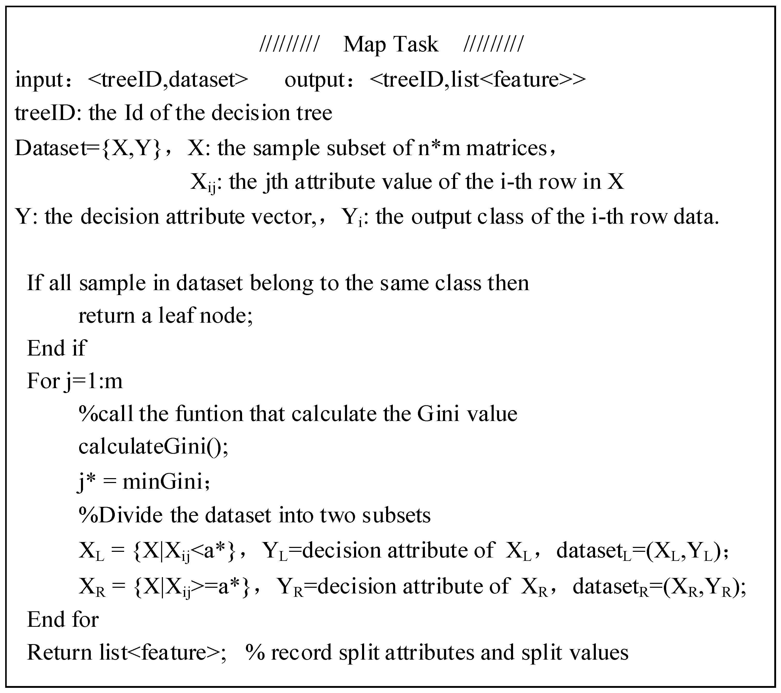
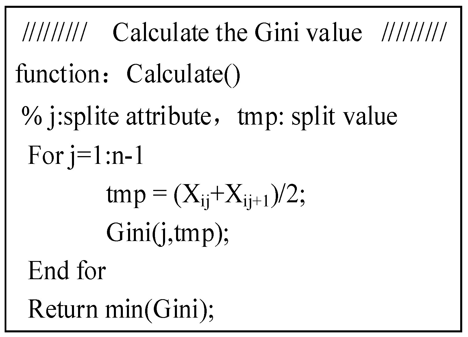
The input of the Map function is <treeID, dataset>. This function mainly completes the decision tree construction, and the output is <treeID, list<feature>>. MapReduce parallelism is also used to select the splitting attribute of the node. Every time the non-leaf node selects the split attribute, it needs to calculate the Gini value of the remaining feature attributes, and return the best split attribute and its value by comparison. The pseudo code is shown in Figure 7 and Figure 8.
Step 3: 
All the Map tasks are completed, which means that the construction of the decision tree has been completed. At this time, the Reduce task is executed, and the split rule of each decision tree is written into HDFS to obtain a random forest classifier.

4.2. Implementation of Neural Network Algorithm Based on MapReduce

Parallelization of the back propagation (BP) neural network model achieves parallelization of data processing. Multiple compute nodes are deployed on the Hadoop platform, and each node has a complete BP neural network model to process part of the sample data, so the calculation of each node is parallelized. Training the neural network model on the Hadoop platform includes the Map, Reduce, and Combine stages, as shown in Figure 9.
① Map stage
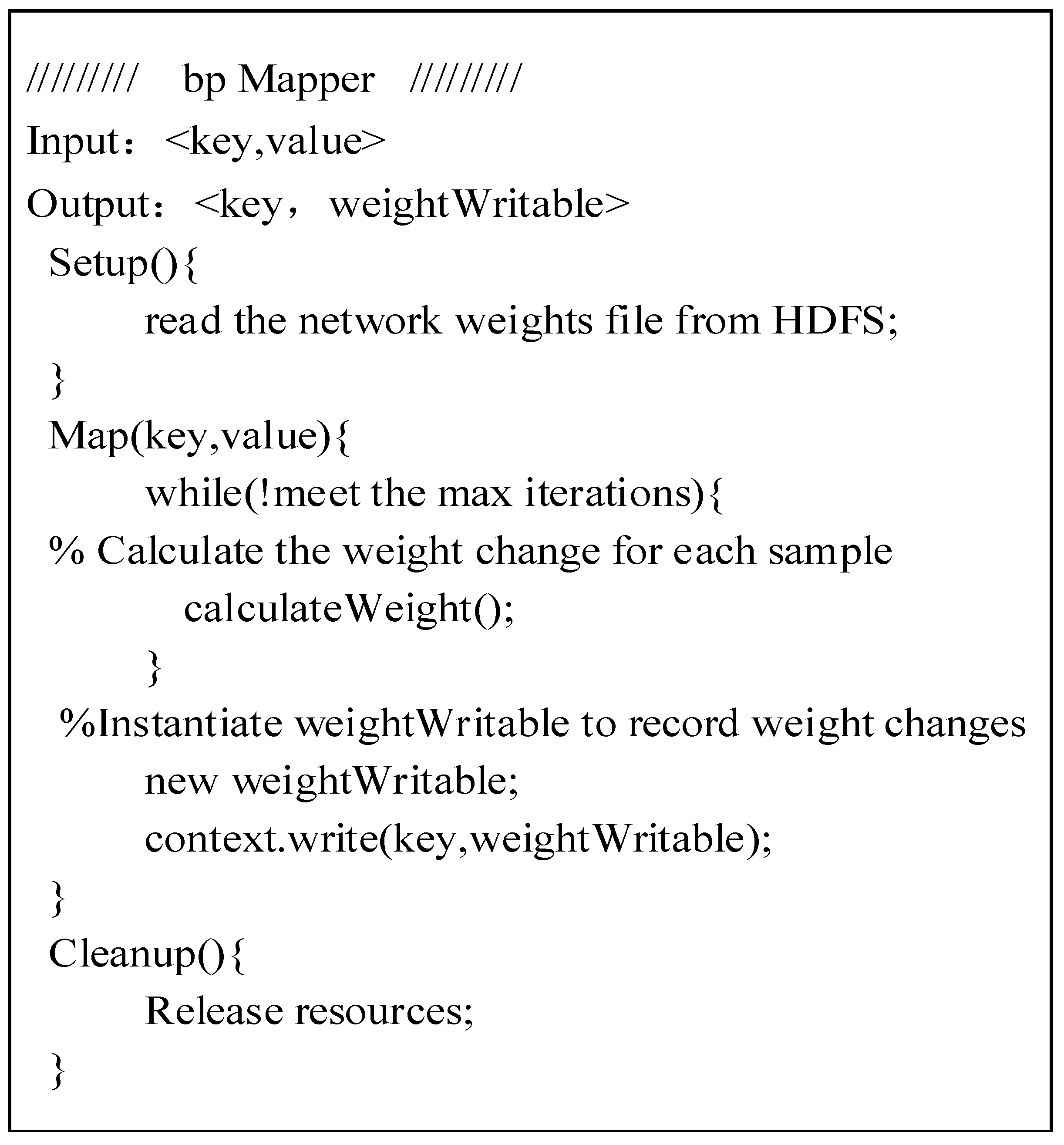
In the Map stage, the setup () function reads the initial network weights from the file system HDFS and initializes the neural network. The Map () function reads the sample data and trains on that node. After the set condition is reached (if the set number of iterations is reached, or the output error reaches the set value, the number of iterations reached in this section is used), and the model training ends. The pseudo code of Map is shown in Figure 10.
② Combine stage
Combine is used to merge the results of the Map. The input is the output of the Map, and its output is the input of Reduce. The type is the same as the output type of Map.
③ Reduce stage
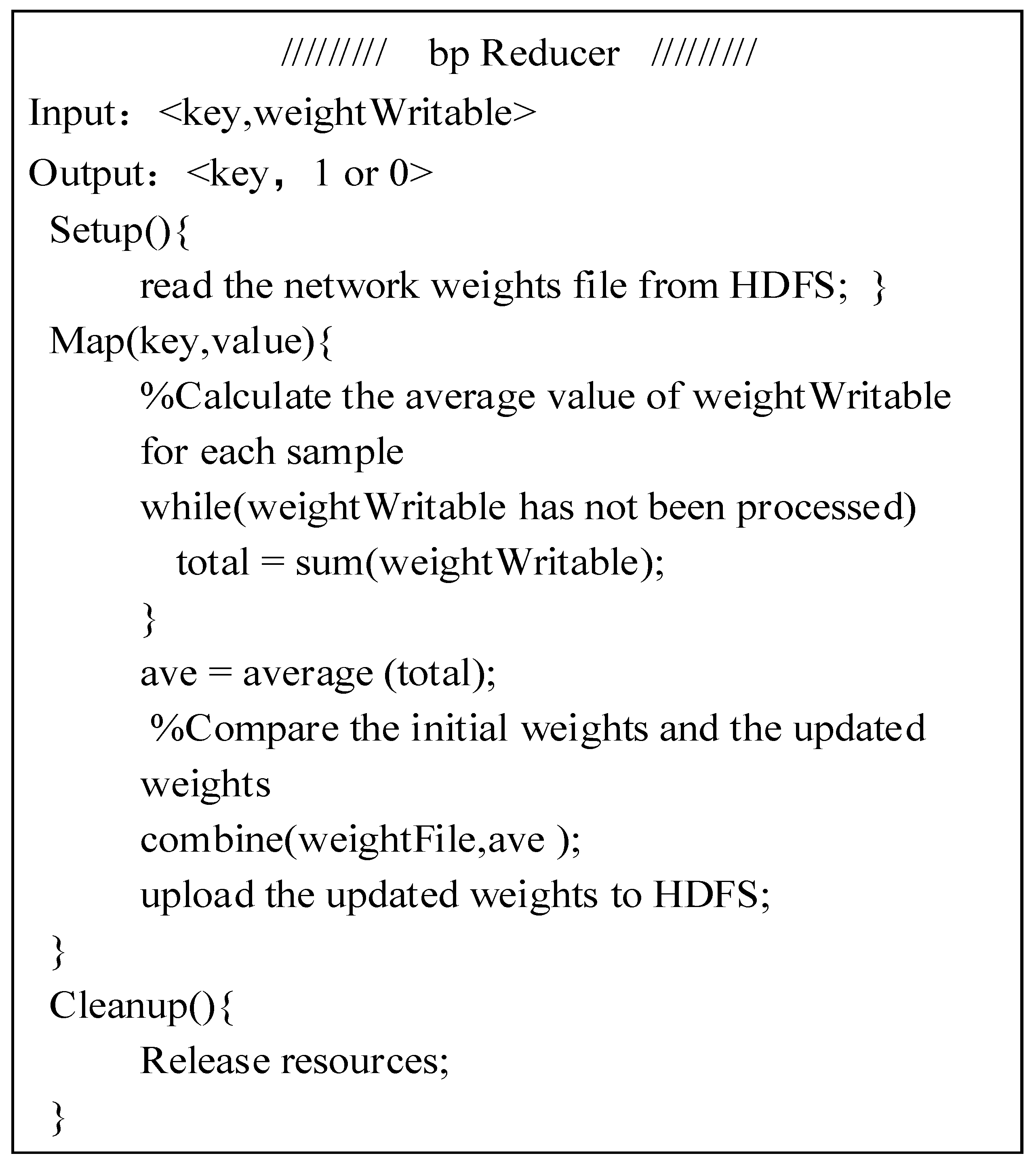
In the Reduce stage, the <key, weightWritable> output of the Combine stage is used as the input of Reduce stage. The Reduce () function is to calculate the average value of the value for each key, and compare it with the network weight stored on the HDFS to determine whether to perform the next loop operation, and finally re-write the updated weights to HDFS. The pseudo code of Reduce stage is shown in Figure 11.

4.3. Fault Diagnosis Experiment of SF6 Electrical Equipment

4.3.1. Experimental Programming

Two MapReduce tasks are set up on the Hadoop platform to diagnose SF6 electrical equipment, as shown in Figure 12. In the first task MR1, the random forest model is used for initial diagnosis. In the second task MR2, the neural network model is used for diagnosis of fault categories.
MR1 is mainly divided into Map and Reduce stages, namely:
(1)
Map stage
Setup () loads the random forest file in HDFS.
Enter the sample to be diagnosed for the first level of diagnosis and statistically determine the diagnosis result of the decision tree.
Output <key, value>, where the key is the flag of whether the sample may be fault data. If the key is 1, it means the sample is normal data. If the key is 2, it means that the majority of the decision tree is abnormal for the diagnosis of the sample; the value is the sample data and the diagnosis result.
(2)
Reduce stage
Enter the output of the Map stage.
Use different files for different key values to save, where the key is 1 and the data is saved in a file named normal, no further processing is required. The data with key 2 is stored in a file named input2 as the input file for the second job.
The MapReduce process of MR2 is as follows:
(1)
Map stage
Use the setup () to initialize the met matrix object, import the weight matrix of each layer of the trained neural network, and build a neural network model.
The input data in map () is the input2 file data of MR1, and the sample is judged to obtain the diagnosis result. The reliability of the diagnosis result is calculated.
Output <key, value>, where the key is the flag for successful diagnosis. If the key is 1, it indicates that the reliability of the diagnosis result of the sample reaches the set credibility threshold requirement, otherwise the credibility threshold is not reached; the value is the sample data and the diagnosis result.
Close the met object in cleanup ().
(2)
Reduce stage
Enter the output of the Map stage.
Save different files for different key values, where a key of 1 means no further processing is required and the result is saved directly. Data with a key of 2 requires expert re-diagnosis and is stored in a file called to Expert.

4.3.2. Experimental Results and Analysis

(1) Verify the validity of the model.
There are three types of faults in SF6 electrical equipment: arc, spark and corona discharge. In this experiment, normal data and data including arc and corona discharge are sent to the model for training, and then the monitoring data including spark discharge is diagnosed.
① Random forest model results.
First, 70% of the 2000 samples (10% of which are fault data and the rest are normal data) are used to train the random forest model, and 30% (including 60 sets of data is fault data) are used to test the model. After testing, the results are shown in Table 8, where category 1 is fault data and category 2 is normal data.
As can be seen from Table 8, one piece of data is normal, but it is classified as possible fault data. All fault data can be identified. From the results of the diagnosis, the random forest model can distinguish between normal and fault data.
② Neural network model results.
70% of the samples were used to train the neural network model, and 30% of the samples were used to test the model. Some diagnostic results are shown in Table 9.
The reliability of the sample diagnosis shown in Table 9 is greater than the set confidence threshold (threshold is 0.8), so the neural network model is considered to be able to determine the diagnosis. In practice, the samples numbered 58 and 61 are the monitoring data when corona discharge occurs, and the samples numbered 64 and 99 are the monitoring data when the arc discharge occurs, so the diagnosis result is correct.
③ Monitoring data diagnosis results and analysis.
After training the model, 10,010 groups (10,000 normal data and 10 sets of fault data) to be diagnosed into the diagnostic model, after the random forest diagnosis model, all 10 groups of fault data are identified, and after the neural network model is substituted, the diagnosis is made. The results are shown in Table 10.
It can be seen from Table 10, the credibility of samples 5 and 6 is less than the threshold (threshold is 0.8), so they are sent to experts for evaluation. They have been identified as a new fault type—spark discharge. Then the neural network model is retrained and the network weights are updated so that the model can identify the type of spark discharge. The diagnosis results of the updated neural network model for samples Nos. 5 and 6 are shown in Table 11.
It can be seen from Table 11 that the reliability of the sample diagnosis results of the numbers 5 and 6 is greater than threshold, that is, the updated neural network model can accurately diagnose the new fault type.
(2) Experiment 2: Comparison of fault diagnosis performance between Stand-alone and cluster mode.
The speedup S is usually used to measure the performance of parallel algorithms, which are defined as follows:
S = T s T m
where T s is the time taken for diagnosis by one node, T m is the time taken for nodes to perform parallel operations.
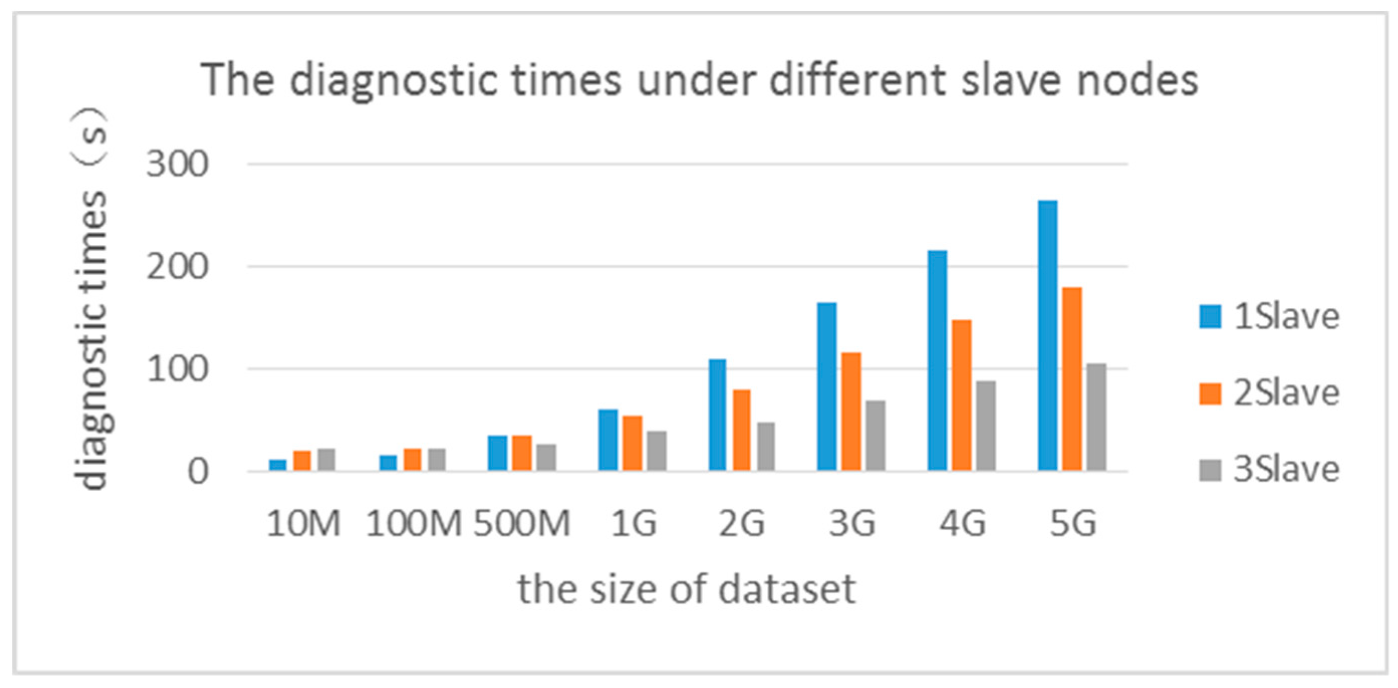
The datasets of different sizes are run in the cluster mode of the Hadoop platform. The diagnostic times under different slave nodes are shown in Table 12.
In order to more intuitively compare the speed of the fault diagnosis algorithm, the Table 12 is converted into a histogram as shown in Figure 13. It can be seen from Figure 13 that when the size of data to be diagnosed is less than 500 MB, the time consumed by single node and multiple nodes is similar. But as the size increases, the time of the fault diagnosis system in a stand-alone model is longer than cluster model. Therefore, when the size of the data that needs to be diagnosed reaches a certain level, using Hadoop’s cluster mode can greatly improve the speed of fault diagnosis.
Through calculation, the speedup of fault diagnosis under different node numbers is shown in Table 13. It can be seen that when the amount of data to be diagnosed is small (less than 500 MB in the experiment), the acceleration ratio of the diagnosis is less than 1, indicating that the operating efficiency of cluster mode is lower than the stand-alone at this time. However, when the amount of data increases, with the increase in the number of nodes, the speedup also increases.
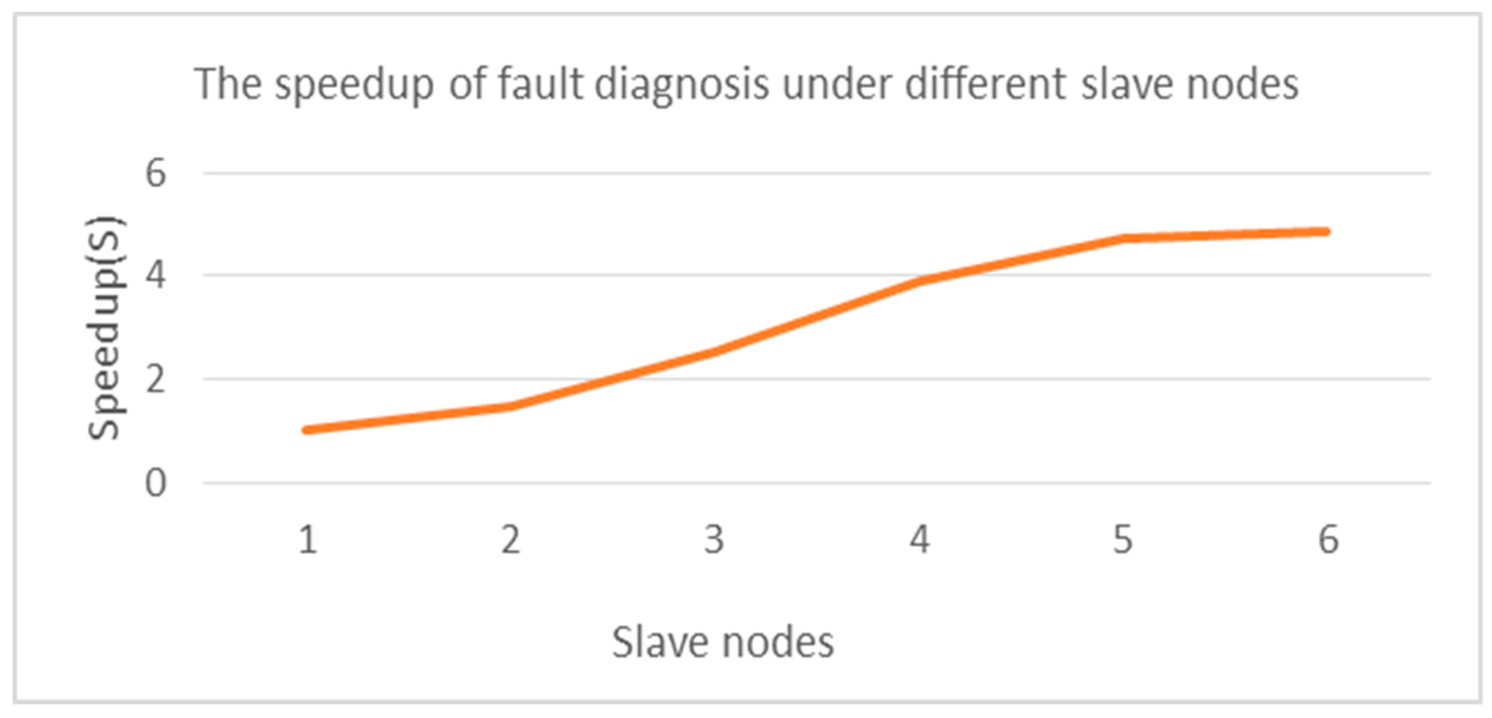
In order to further compare the influence of the number of nodes on the diagnosis speed, the experiment was carried out for the case where the data amount was 5 GB, and the result is shown in Figure 14.
As can be seen from Figure 14, when the amount of data is 5 GB, the speedup does not increase linearly with the increase in the number of nodes. This is because as the cluster size increases, the time spent communicating between nodes increases. Therefore, in practice, the size of the cluster can be selected according to the size of the amount of data.

5. Conclusions

In this paper, a two-level fault diagnosis model for SF6 electrical equipment is designed, and fault diagnosis for SF6 electrical equipment is implemented on the Hadoop platform in this paper. Before training the fault diagnosis model, the monitoring data is preprocessed first, and different data filling methods are adopted for different missing values. Secondly, the fault diagnosis algorithms are parallelized on the Hadoop platform. Finally, the time consumption of fault diagnosis of SF6 electrical equipment in stand-alone mode and cluster mode is compared by simulation, and the advantages of cluster mode in processing massive data are verified.
The first-level diagnostic model can quickly diagnose monitoring data and filter out the problematic data in a large amount of data. The second-level diagnostic model provides an in-depth analysis of the fault types of SF6 electrical equipment and can be learned in real time to update the fault type library.
In the future, smart substations can be equipped with SF6-derived gas composition detection equipment (such as infrared spectrum analyzers) and upload data to cloud databases in real time. Engineers can check the operating status of SF6 electrical equipment in real time on the client side, which saves time in field inspections. Engineers can quickly and accurately identify problems to avoid security incidents.

Author Contributions

All authors have equally contributed substantially to the work reported. Conceptualization, H.M.; Data curation, H.Z.; Formal analysis, H.Z.; Funding acquisition, B.Q.; Investigation, M.C.; Methodology, H.M.; Project administration, H.M.; Resources, M.C. and J.L.; Software, H.Z. and J.L.; Supervision, H.M.; Visualization, H.Z. and B.Q.; Writing—original draft, H.Z.; Writing—review and editing, M.C.

Funding

This paper is supported by the national Natural Science Foundation of China (51607057). The authors also gratefully acknowledge the helpful comments and suggestions of the reviewers, which have improved the presentation.

Conflicts of Interest

The authors declare no conflict of interest.

References

  1. Li, M.C.; Wang, Y.P. Smart substation and technical characteristics analysis. Power Syst. Prot. Control 2010, 38, 59–62. [Google Scholar]
  2. Liu, M. Electrical Device Failure Diagnosis Research Based on the Analysis of the SF6 Gas Decomposition; Hunan University: Changsha, China, 2013. [Google Scholar]
  3. Chu, F.Y. SF6 Decomposition in Gas-Insulated Equipment. IEEE Trans. Electr. Insul. 1986, EI-21, 693–725. [Google Scholar] [CrossRef]
  4. Christophorou, L.G.; Olthoff, J.K. Sulfur hexafluoride and the electric power industry. IEEE Electr. Insul. Mag. 1997, 13, 20–24. [Google Scholar] [CrossRef]
  5. Cai, T. Research on SF6 Electric Equipments’ Fault Diagnosis and Precaution Based on SF6’s Ramifications; Wuhan University: Wuhan, China, 2011. [Google Scholar]
  6. Ray, J.; Johnny, O.; Trovati, M.; Sotiriadis, S.; Bessis, N. The Rise of Big Data Science: A Survey of Techniques, Methods and Approaches in the Field of Natural Language Processing and Network Theory. Big Data Cogn. Comput. 2018, 2, 22. [Google Scholar] [CrossRef]
  7. Murtagh, F.; Devlin, K. The Development of Data Science: Implications for Education, Employment, Research, and the Data Revolution for Sustainable Development. Big Data Cogn. Comput. 2018, 2, 14. [Google Scholar] [CrossRef]
  8. Kollenstart, M.; Harmsma, E.; Langius, E.; Andrikopoulos, V.; Lazovik, A. Adaptive provisioning of heterogeneous cloud resources for big data processing. Big Data Cogn. Comput. 2018, 2, 15. [Google Scholar] [CrossRef]
  9. 5Apache Hadoop. Available online: http://hadoop.apache.org/ (accessed on 25 October 2018).
  10. Gao, S.; Li, L.; Li, W.; Janowicz, K.; Zhang, Y. Constructing gazetteers from volunteered big geo-data based on Hadoop. Comput. Environ. Urban Syst. 2017, 61, 172–186. [Google Scholar] [CrossRef]
  11. Dean, J.; Ghemawat, S. MapReduce: Simplified data processing on large clusters. Commun. ACM 2008, 51, 107–113. [Google Scholar] [CrossRef]
  12. Dean, J.; Ghemawat, S. MapReduce: A flexible data processing tool. Commun. ACM 2010, 53, 72–77. [Google Scholar] [CrossRef]
  13. Flaishans, J.; Fry, M.; Hook, T.; Thurman, N.; Carleton, J.; Thawley, S.; Wolfe, K.; Young, D.; Purucker, T. Scaling Watershed Models: Modern Approaches to Science Computation with MapReduce, Parallelization, and Cloud Optimization. In Proceedings of the 8th International Congress on Environmental Modelling and Software, Toulouse, France, 11–14 July 2016. [Google Scholar]
  14. Suehiro, J.; Zhou, G.; Hara, M. Detection of partial discharge in SF6 gas using a carbon nanotube-based gas sensor. Sensors Actuators B: Chem. 2005, 105, 164–169. [Google Scholar] [CrossRef]
  15. Manion, J.P.; Philosophos, J.A.; Robinson, M.B. Arc stability of electronegative gases. IEEE Trans. Electr. Insul. 1967, EI-2, 1–10. [Google Scholar] [CrossRef]
  16. Belmadani, B.; Casanovas, J.; Casanovas, A.M.; Grob, R.; Mathieu, J. SF/sub 6/decomposition under power arcs. I. Physical aspects. IEEE Trans. Electr. Insul. 1991, 26, 1163–1176. [Google Scholar] [CrossRef]
  17. Sauers, I.; Ellis, H.W.; Christophorou, L.G. Neutral decomposition products in spark breakdown of SF6. IEEE Trans. Electr. Insul. 1986, EI-21, 111–120. [Google Scholar] [CrossRef]
  18. Xiao, X.; Miao, H.; Li, M.; Qi, B. The two-level fault diagnosis model of SF 6 electrical equipment. In Proceedings of the 2017 3rd IEEE International Conference on Computer and Communications (ICCC), Chengdu, China, 13–16 December 2017; pp. 2868–2872. [Google Scholar]
  19. Stuart, B. Infrared spectroscopy. Kirk-Othmer Encycl. Chem. Technol. 2005. [Google Scholar] [CrossRef]
  20. Kurte, R.; Beyer, C.; Heise, H.; Klockow, D. Application of infrared spectroscopy to monitoring gas insulated high-voltage equipment: Electrode material-dependent SF6 decomposition. Anal. Bioanal. Chem. 2002, 373, 639–646. [Google Scholar] [CrossRef] [PubMed]
  21. Heise, H.M.; Kurte, R.; Fischer, P.; Klockow, D.; Janissek, P.R. Gas analysis by infrared spectroscopy as a tool for electrical fault diagnostics in SF6 insulated equipment. Fresenius’ J. Anal. Chem. 1997, 358, 793–799. [Google Scholar] [CrossRef]
  22. Li, X.F. Research and Application of Data Preprocessing Algorithm; Southwest Jiaotong University: Chengdu, China, 2006. [Google Scholar]
Figure 1. System block diagram for fault diagnosis of SF6 electrical equipment.
Bdcc 03 00004 g001
Figure 2. Flow chart of two-level fault diagnosis algorithm.
Bdcc 03 00004 g002
Figure 3. Architecture of the two-level fault diagnosis system for SF6 electrical equipment.
Bdcc 03 00004 g003
Figure 4. The data interpolation process based on method of grey correlation.
Bdcc 03 00004 g004
Figure 5. The parallel forest construction process of random forest.
Bdcc 03 00004 g005
Figure 6. The specific tree construction process in Map task.
Bdcc 03 00004 g006
Figure 7. The pseudo code to construct a decision tree in Map task.
Bdcc 03 00004 g007
Figure 8. The pseudo code to calculate Gini value.
Bdcc 03 00004 g008
Figure 9. The process of training back propagation (BP) neural network model.
Bdcc 03 00004 g009
Figure 10. The pseudo code of Map stage.
Bdcc 03 00004 g010
Figure 11. The pseudo code of Reduce stage.
Bdcc 03 00004 g011
Figure 12. The diagnosis process of SF6 electrical equipment.
Bdcc 03 00004 g012
Figure 13. The diagnostic times under different slave nodes.
Bdcc 03 00004 g013
Figure 14. The speedup of fault diagnosis under different slave nodes.
Bdcc 03 00004 g014
Table 1. The historical data of SOF2.
Id1234567
Value5.46.86.56.96.75.95.1
Table 2. The interpolation results of SOF2.
IdMIMWIMThe Error of MIMThe Error of WIM
36.456.530.00770.0046
46.4756.500.06160.0580
56.106.160.08960.0806
Note: MIM means mean interpolation method, WIM means weighted interpolation method.
Table 3. The historical data of SOF.
Id1234567
Value43.242.145.341.944.842.851.1
Table 4. The interpolation results of SOF2.
IdMIMWIMThe Error of MIMThe Error of WIM
342.5042.400.06180.0640
442.6542.930.01790.0246
544.67543.970.04380.0273
Table 5. The historical data of SOF2.
Id1234567
Value8.88.38.612.916.215.318.2
Table 6. The interpolation results of SOF2.
Id34
Method
MIM11.5512.10
WIM (weight: 0.2, 0.3)11.3612.16
WIM (weight: 0.125, 0.375)11.0712.25
WIM (weight: 0.125, 0.375)0.34300.0620
The error of WIM (weight: 0.2, 0.3)0.32090.0574
The error of WIM (weight: 0.125, 0.375)0.28720.0539
Table 7. The results of interpolating missing values.
IdThe Top 10 Values of RelevanceInterpolated ValueError
38.2, 8.5, 9.1, 8.3, 8.3, 8.6, 9.5, 7.9, 8.2, 8.58.510.01
410.8, 11.5, 13.4, 12.3, 14.2, 15.6, 11.8, 12.9, 17.2, 13.513.320.033
Table 8. The test results of random forest model.
Target Category 1Target Category 2
Number of diagnostic category 1601
Number of diagnostic category 20539
Table 9. Some diagnostic results of neural network model.
Sample NumberNormalCorona DischargeArc DischargeCredibility
580.0031−0.00190.99140.9950
610.00120.00510.99500.9937
640.00631.00190.00130.9925
990.00160.99330.00740.9910
Table 10. The results of neural network model.
NumberNormalArc DischargeCorona DischargeCredibility
1−0.00150.00190.99880.9966
20.0024−0.00730.99820.9904
30.0056−0.00260.99880.9919
4−0.0021−0.00740.98720.9905
50.01790.67400.32430.6633
60.02610.52710.47210.5141
7−0.00411.00120.00190.9940
8−0.00111.00080.00850.9905
90.00631.00100.00870.9852
100.00191.00090.00470.9966
Table 11. The diagnosis results of the updated neural network model.
NumberNormalSpark DischargeArc DischargeCorona DischargeCredibility
50.00190.99720.00890.01360.9761
60.00080.9988−0.00880.00190.9886
Table 12. The diagnostic times under different slave nodes.
Number10 MB100 MB500 MB1 GB2 GB3 GB4 GB5 GB
1 Slave10.215.235.460.2110165.3215265.5
2 Slave19.621355480116.3148178.6
3 Slave21212539.64769.288.5104.2
Table 13. The speedup of fault diagnosis under different node numbers.
Speedup10 MB100 MB500 MB1 GB2 GB3 GB4 GB5 GB
1 Slave11111111
2 Slave0.520.721.011.111.381.421.451.49
3 Slave0.480.721.411.522.342.392.432.55