DL-VLM: A Dynamic Lightweight Vision-Language Model for Bridge Health Diagnosis

Abstract

Bridge health diagnosis plays a vital role in ensuring structural safety and extending service life while reducing maintenance costs. Traditional structural health monitoring approaches rely on sensor-based measurements, which are costly, labor-intensive, and limited in coverage. To address these challenges, we propose a three-phase solution that integrates the Dynamic Lightweight Vision-Language Model (DL-VLM), domain adaptation, and knowledge-enhanced reasoning. First, as the core of the framework, the DL-VLM consists of three components: a visual information encoder with multi-scale feature selection, a text encoder for processing inspection-related language, and a multimodal alignment module. Second, to enhance practical applicability, we further introduce domain-specific fine-tuning on the Bridge-SHM dataset, enabling the model to acquire specialized knowledge of bridge construction, defects, and structural components. Third, a knowledge retrieval augmentation module is incorporated, leveraging external knowledge graphs and vector-based retrieval to provide contextually relevant information and improve diagnostic reasoning. Experiments on high-resolution bridge inspection datasets demonstrate that DL-VLM achieves competitive diagnostic accuracy while substantially reducing computational cost. The combination of domain-specific fine-tuning and knowledge augmentation significantly improves performance on specialized tasks, supporting efficient and practical deployment in real-world structural health monitoring scenarios.

1. Introduction

Structural health monitoring (SHM) is essential for ensuring structural safety and service longevity, as it enables early detection of aging, material degradation, and environmental damage, thereby reducing maintenance costs and preventing catastrophic failures. Traditional SHM approaches, including manual inspection and sensor-based monitoring, are limited by labor costs and restricted spatial coverage. In response, vision-based methods, especially those driven by deep learning [1,2], have gained increasing attention due to their ability to capture rich visual information from large-scale bridge inspections. However, these methods usually ignore the engineer’s intention and the knowledge of bridge engineering which are described in text information. Recent studies highlight the critical importance of structural context; for example, in Italy alone, 246 partial and total bridge collapses were recorded between 2000 and 2023 [3], emphasizing the urgent need for advanced monitoring techniques that can detect damage early and reason across multiple modalities. To address the limitations of conventional visual approaches in understanding complex structural contexts and leveraging textual engineering knowledge, vision-language models (VLMs) have recently been introduced into bridge health monitoring [4] to enable multimodal reasoning and more interpretable diagnostics.

However, despite the strong capability of current VLMs in handling multimodal information [5], several challenges remain in applying vision-based methods for bridge health diagnosis. First, bridge damage exhibits substantial variability in scale, morphology, and context [6,7], which requires robust multi-scale feature representation while encoding the visual information. Second, the VLMs have demonstrated powerful multimodal reasoning capabilities, but existing models are often large and computationally intensive [8], restricting their deployment in practical SHM scenarios. Third, conventional cross-modal alignment methods typically rely on linear projections, which inadequately capture complex nonlinear interactions between visual features and domain-specific textual descriptions [9], limiting diagnostic accuracy and interpretability.

To address the limitations of existing vision–language models in bridge health diagnosis, the proposed framework integrates three key modules. First, we develop a Dynamic Lightweight Vision–Language Model that employs multi-scale visual feature fusion and adaptive compression to effectively handle large-resolution bridge imagery. This design enhances the model’s ability to capture fine-grained structural cues while maintaining high computational efficiency. Second, to better adapt the model to real-world engineering scenarios, a domain-specific fine-tuning module is introduced, enabling the system to learn specialized knowledge of bridge structures, defect types, and inspection terminology from the Bridge-SHM dataset. This targeted optimization enhances cross-domain generalization and improves diagnostic reliability in complex environments. Third, a knowledge-augmentation module integrates external knowledge graphs and retrieval-based semantic enrichment to supplement the model’s reasoning process with contextually relevant engineering information. By combining lightweight visual modeling, domain-adaptive optimization, and knowledge-driven enhancement, the proposed framework delivers a more robust, interpretable, and practically deployable solution for bridge health monitoring.

2. Related Work

2.1. Technical Background for Bridge Health Monitoring

SHM of bridges has been studied using vibration-based sensing, visual inspection, and image analysis [10]. The sensor-based methods can monitor the micro-defects and dynamic risks of bridges in real time and reduce potential safety hazards. However, it has high installation and maintenance costs, is susceptible to environmental interference and is difficult for widespread implementation [11]. Traditional vision-based methods can detect cracks, corrosion, and spalling but are sensitive to noise and lack robustness in complex environments [12]. With the success of deep learning, CNN- and RNN-based approaches have been adopted for automated bridge damage detection and classification recently [13,14]. In particular, recent work has demonstrated real-time crack detection and prediction using hybrid architectures combining CNN, U-Net, and Swin Transformer, achieving high precision on structural crack segmentation tasks [15].

Additionally, systematic reviews of AI-based SHM for existing bridges have highlighted not only visual inspection and sensor data processing but also future opportunities for digital twin integration, predictive maintenance, and continuous risk assessment [16]. digital twin-based anomaly detection systems integrating SHM, finite element modeling, and bridge information modeling have been systematically reviewed to highlight their potential for structural damage monitoring [17]. While these models improve detection accuracy, they rely heavily on large-scale labeled data and cannot capture multimodal contextual information of bridge knowledge, limiting their generalization in practical SHM scenarios [18].

The Vision Transformer (ViT) [19] extends the Transformer architecture from natural language processing to image understanding. The core idea of ViT is to treat an image as a sequence of visual tokens by dividing it into fixed-size patches, thereby enabling global dependency modeling through self-attention mechanisms. This approach replaces traditional convolutional operations with a token-based encoding to better capture long-range relationships across the entire image.Through this mechanism, ViT models global contextual dependencies among image patches, providing a unified and flexible framework for visual representation learning. The main advantage of ViT is its ability to capture both local and global features without explicit inductive biases such as translation equivariance. However, ViT becomes computationally expensive when applied to high-resolution images, since the self-attention operation scales quadratically with the number of patches, making it less suitable for fine-grained bridge inspection tasks that require detailed structural analysis.

Building upon joint vision–language representation learning, Radford et al. [20] proposed the Contrastive Language–Image Pretraining (CLIP) model. CLIP learns a shared embedding space for images and text by aligning them through contrastive learning on 400 million image–text pairs collected from the web. This enables strong zero-shot generalization, as the model can associate textual descriptions with previously unseen visual content. Despite its impressive cross-modal understanding capability, CLIP’s reliance on large-scale paired data poses challenges for reproducibility and adaptation to specialized domains like bridge health monitoring, where data scarcity and domain shift are common.

To improve multimodal alignment efficiency, Liu et al. [21,22] developed the Large Language and Vision Assistant (LLaVA) model, which integrates a visual encoder (e.g., CLIP ViT backbone) with a large language model through lightweight projection layers. This design enables end-to-end alignment between visual and linguistic modalities using a much smaller number of paired samples. LLaVA demonstrates strong instruction-following ability and effective multimodal reasoning with limited data. However, its reasoning on fine-grained visual cues remains limited due to the relatively small scale of its aligned supervision, which can be particularly restrictive in detecting subtle structural damages on bridge surfaces.

Li et al. [9] proposed the Query Transformer (Q-Former) as a mechanism to efficiently bridge visual and textual modalities. Q-Former introduces a set of learnable queries that interact with dense image tokens, extracting compact yet informative representations. By reducing the number of visual tokens passed to the language model, Q-Former significantly lowers computational cost during inference. This token compression mechanism enhances inference efficiency but may lead to the loss of critical fine-grained information—an issue of particular concern for tasks such as structural damage localization in bridge health monitoring, where subtle features like cracks or corrosion patterns are diagnostically crucial.

Beyond VLMs, efficiency improvements have been explored through techniques such as dynamic sampling, and multi-scale feature fusion [23,24,25]. Dynamic sampling further adapts the processing by selectively focusing on regions of interest in an image, allowing models to allocate more resources to critical areas while ignoring redundant or background regions [23]. Multi-scale feature fusion combines information from different spatial resolutions, improving the model’s ability to capture both global context and local fine details [25]. These approaches have demonstrated significant computational savings and performance gains in generic vision tasks. However, when applied to domain-specific scenarios such as bridge health monitoring, caution is needed: damage regions are sparse yet crucial, and discarding tokens indiscriminately may impair diagnostic reliability [26].

2.2. Technical Background for Model Fine-Tuning and Knowledge Enhancement

LoRA [27] is an efficient parameter-efficient fine-tuning technique widely used for adapting Large Language Models (LLMs) and VLMs. Instead of updating the full set of model parameters—which is computationally expensive—LoRA introduces a small number of trainable low-rank parameters while keeping the original model weights frozen. This significantly reduces memory usage and training cost. Because only a lightweight set of parameters is optimized, LoRA enables fast task adaptation on resource-limited hardware while maintaining model performance. Many variants, such as QLoRA [28] and AdaLoRA [29], further enhance efficiency through quantization or adaptive rank selection. With these advantages, LoRA has become a mainstream solution for fine-tuning open-source LLMs in practical deployments.

However, efficient fine-tuning alone is not sufficient for domain-specific tasks that require external knowledge or large-scale information access. To address this, a retrieval module is introduced to supply the model with relevant contextual information. Dense Passage Retrieval (DPR) [30] serves this purpose by identifying semantically relevant documents from large corpora. DPR encodes queries and documents into dense embeddings using two encoders and retrieves the nearest neighbors from a prebuilt vector index. Its ability to capture semantic similarity beyond lexical overlap makes it highly effective for large-scale question answering and knowledge retrieval.

While DPR offers strong recall, the retrieved candidates may still include noisy or weakly related passages. To improve precision, a second-stage reranking step is applied. These rerankers typically use cross-encoder architectures [31], in which the query and each candidate passage are jointly encoded to compute a more accurate relevance score. Although cross-encoders are computationally heavier than bi-encoders, applying them only to the Top-K results provides a good balance between efficiency and accuracy, significantly enhancing the final quality of retrieval-based downstream tasks.

3. Methodology

3.1. Overall Framework

The proposed framework comprises three core components which integrates a general dynamic leightweight visual-language understanding with domain-specific expertise and external knowledge support. First, the Dynamic Lightweight Vision-Language Model provides a foundation for efficient multimodal representation learning, employing multi-scale feature extraction and adaptive fusion to handle variations in bridge structures and damage patterns. Second, Domain-Specific Fine-Tuning adapts the pretrained model to bridge engineering tasks by leveraging the Bridge-SHM dataset, enabling the model to capture specialized terminology, defect types, and structural nuances. Third, the Knowledge Augmentation module enhances the model’s reasoning capabilities by retrieving relevant information from external knowledge sources, including knowledge graphs and vector-based repositories, to support accurate and context-aware diagnostic outputs. Collectively, these components form a unified framework that balances generalization, domain specialization, and knowledge-enhanced reasoning, providing robust and efficient support for real-world structural health monitoring applications.

3.2. Dynamic Lightweight Vision-Language Model

With processing high-resolution bridge images while maintaining robust multimodal understanding capabilities, the proposed architecture comprises three core components: (a) a multi-scale visual feature extraction and down-sampling module, (b) a cross-modal fusion module with learnable feature projection, and (c) a large language model for multimodal reasoning and decision output.

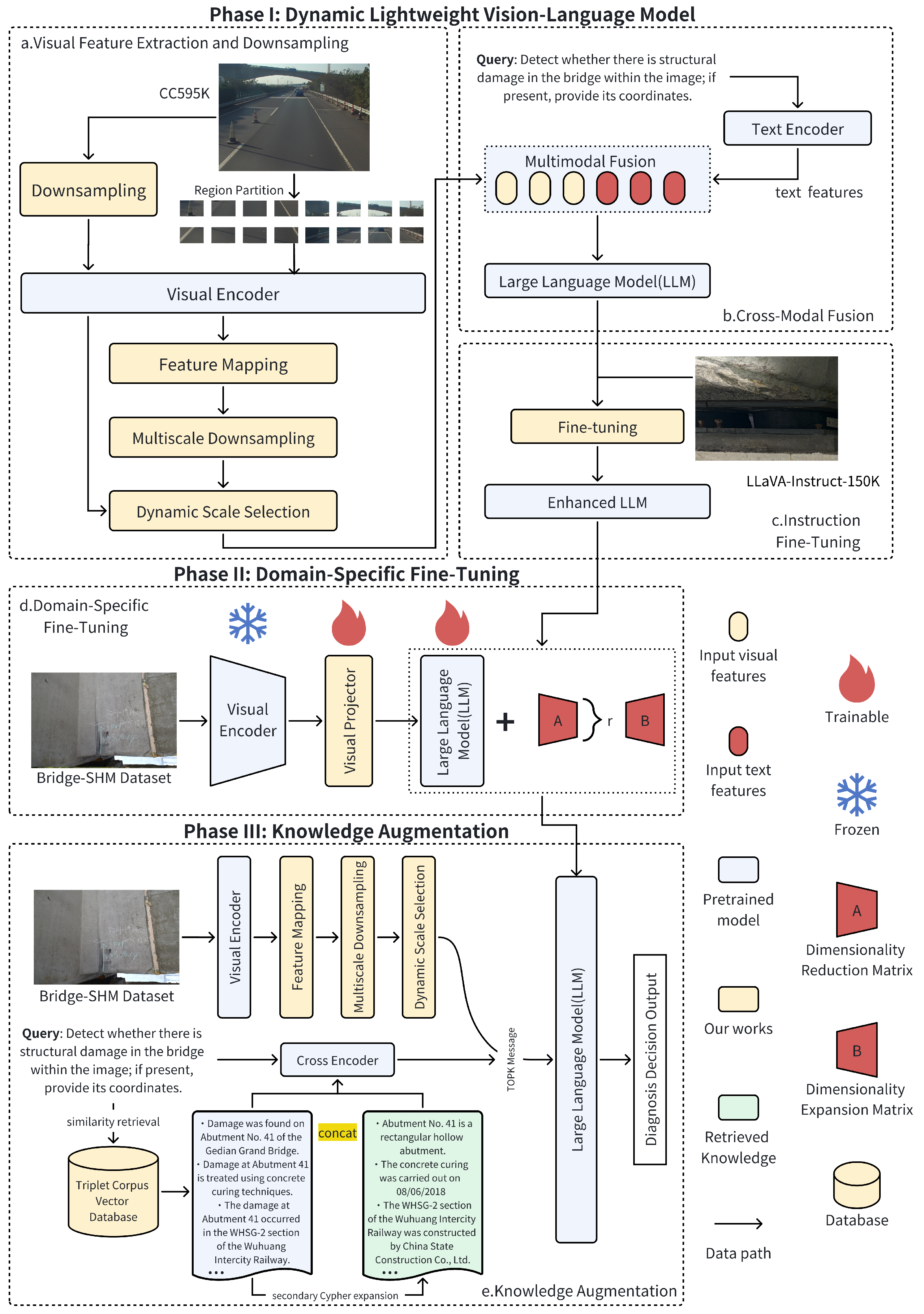
Typically, the feature dimension output by the visual encoder is high (e.g., 1024 for CLIP-ViT-L/16), while the language model’s embedding space is lower (e.g., 768). To process multi-dimensional visual features, a dynamic visual feature down-sampler is designed as a key component of the visual projector. By mapping the high-dimensional visual features into the embedding space of the language model, the visual projector enables alignment and fusion of visual and textual features. Moreover, visual features often contain substantial spatial and texture redundancy. Direct use of raw high-dimensional features not only increases computational burden but may also lead to overfitting. The dynamic visual feature down-sampler mitigates these issues by adaptively compressing features based on their information density, retaining critical semantic information while reducing the total number of features. The structure of the DL-VLM is illustrated in Figure 1a–c.

The model processes high-resolution input images $I\in {\mathbb{R}}^{H\times W\times 3}$ through a hierarchical pipeline. The image is divided into local regions, where structurally dense areas (e.g., bridge piers, cables) are down-sampled conservatively while background regions undergo stronger compression. Visual features are then mapped into the language model’s embedding space via a multi-layer perceptron with Mish activation as the feature mapping block. The language model jointly processes the compressed visual tokens and textual inputs, which are concatenated within the shared embedding space to enable multimodal fusion. A two-stage training strategy, first for cross-modal alignment and then task-specific fine-tuning, ensures both efficiency and fidelity for bridge health diagnosis. The key symbols used in our framework are summarized in

Table A1. Summary of Crucial Notations Used in the Proposed Framework.

Symbol	Meaning
$I_g$	Downsampled global image representation used as input to the global visual encoder.
$v_g$	Global visual embedding generated by the shared-weight ViT encoder from $I_g$.
$X_i$	i-th local image patch or cropped region extracted for fine-grained feature encoding.
$D_j^{\left(i\right)}$	j-th token or feature element in the i-th document/knowledge sequence.
$D{S}^{\left(i\right)}\left[s\right]$	The s-th retrieved semantic sentence associated with the i-th bridge or query instance.
${\hat{X}}_i$	Reconstructed or enhanced representation of the i-th local region (varies by stage of the model).
q	Dense query embedding encoded from the input prompt in the retrieval module.
d	Dense embedding of a knowledge triple or document fragment stored in the vector database.
$L_{\mathrm{balance}}$	Loss term enforcing balance between global and local feature learning objectives.
${\mathcal{T}}_{\mathrm{cand}}$	Candidate triple set obtained by merging DPR-retrieved and graph-expanded triples.
$s_i$	Relevance score assigned by the Cross-Encoder to the i-th triple.

.

3.2.1. Image Region Partitioning

For the input high-resolution image $I\in {\mathbb{R}}^{H\times W\times 3}$, we first partition the region to enable fine-grained local feature extraction. Inspired by the sliding-window based partition strategy proposed in FocusLLaVA [32], the original image I is divided into N local sub-images $I_1,I_2,\dots ,I_N$ of equal size $w\times w$ with either overlapping or non-overlapping regions. The sliding-window approach progressively crops fixed-size windows across the image in a raster-scan fashion, which ensures dense coverage of local regions while preserving spatial consistency. Then, an image sequence is formed as shown in Equation (1):

$$\{I_1,I_2,\dots ,I_N\}=\mathrm{Partition}\left(I\right)$$

(1)

The partition $I_i(i=1,2,\dots ,N)$ is fed into a shared-weight Vision Transformer (ViT) encoder [19] to extract its semantic embedding features:

$$v_i=\mathrm{ImageEncoder}\left(I_i\right)$$

(2)

So the series of local feature blocks is obtaind as shown in Equation (3):

$$\{v_1,v_2,\dots ,v_N\}$$

(3)

The window size of each region is denoted as $w\in \mathbb{N}$, and each feature block $v_i$ serves as the basic processing unit. Here $i=1,2,\dots ,N$ and $N=H/w\times W/w$. The image encoder adopts the patch embedding mechanism of the original ViT architecture, where each input image is uniformly divided into fixed-size patches that are linearly projected into token embeddings before being processed by the transformer layers.

Meanwhile, the entire image is retained and downsampled into feature maps $I_g$ of size $w\times w$. The resulting $I_g$, representing the global visual feature, is then fed into the shared weight ViT encoder to generate the global embedding $v_g$, as shown in Equation (4):

$$v_g=\mathrm{ImageEncoder}\left(I_g\right)$$

(4)

3.2.2. Feature Mapping with Mish Activation

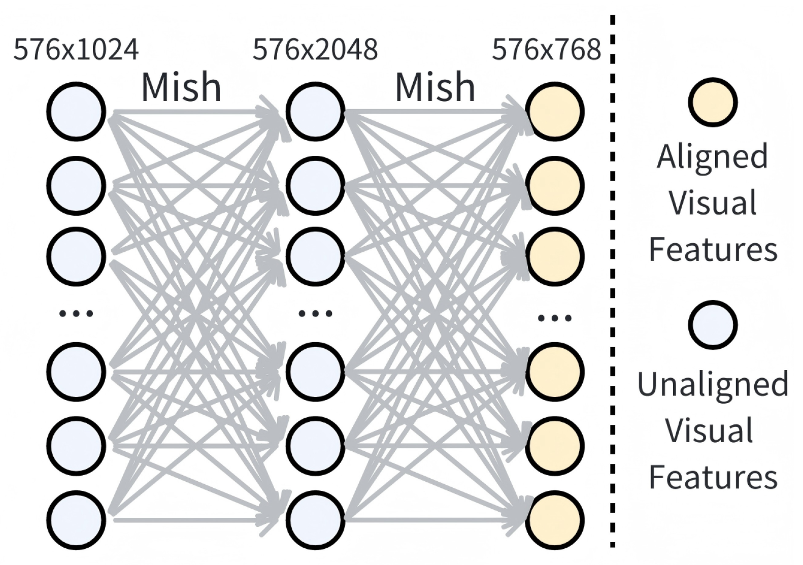
To enhance the expressive power of visual features in multimodal tasks, we employ the Multi-Layer Perceptron (MLP) [33] and the Mish activation function [34] to strengthen the model’s nonlinear modeling capability, as illustrated in Figure 2. Unlike traditional ReLU [35] or GELU [36] activations, Mish is a smooth and non-monotonic activation function that preserves negative value information while possessing stronger gradient flow, demonstrating superior performance in various visual tasks.

In the feature mapping stage, the feature vectors output by the visual encoder $v_i\in {\mathbb{R}}^{576\times 1024}$ are represented as 576 embedding vectors of length 1024. These features are then fed into a two-layer MLP for nonlinear transformation, ultimately outputting visual tokens $X_i\in {\mathbb{R}}^{576\times 768}$, which will serve as input for subsequent modules to drive multimodal information interaction, as shown in Equations (5) and (6).

$$H_1=\mathrm{Mish}(v_i{W}_1+b_1),\hspace{1em}{W}_1\in {\mathbb{R}}^{1024\times 2048},b_1\in {\mathbb{R}}^{2048}$$

(5)

$$X_i=\mathrm{Mish}(H_1{W}_2+b_2),\hspace{1em}{W}_2\in {\mathbb{R}}^{2048\times 768},b_2\in {\mathbb{R}}^{768}$$

(6)

where $W_1\in {\mathbb{R}}^{1024\times 2048}$ is the weight matrix of the first layer, $W_2\in {\mathbb{R}}^{2048\times 768}$ is the weight matrix of the second layer, $b_1\in {\mathbb{R}}^{2048}$ is the bias vector of the first layer, and $b_2\in {\mathbb{R}}^{768}$ is the bias vector of the second layer.

In this process, the first layer’s dimension-raising operation captures potential high-order feature combinations through a wider hidden space, while the introduction of the Mish activation function further enhances the model’s expressive diversity and gradient stability. The second layer compresses the features to a dimension consistent with the original embedding through projection, maintaining consistency with the language model’s input interface.

3.2.3. Multiscale Downsampling Based on Feature Similarity

Traditional visual feature compression strategies, such as uniform sampling or max-pooling, often ignore the non-uniform distribution of visual features in both spatial and semantic dimensions, resulting in the retention of redundant information while eliminating critical details. This is particularly problematic in engineering images, where structured regions (such as bridge piers, steel bars, etc.) are often mixed with background regions (such as sky, ground). Therefore, sampling methods based solely on position or intensity cannot meet the requirements of high-quality visual understanding.

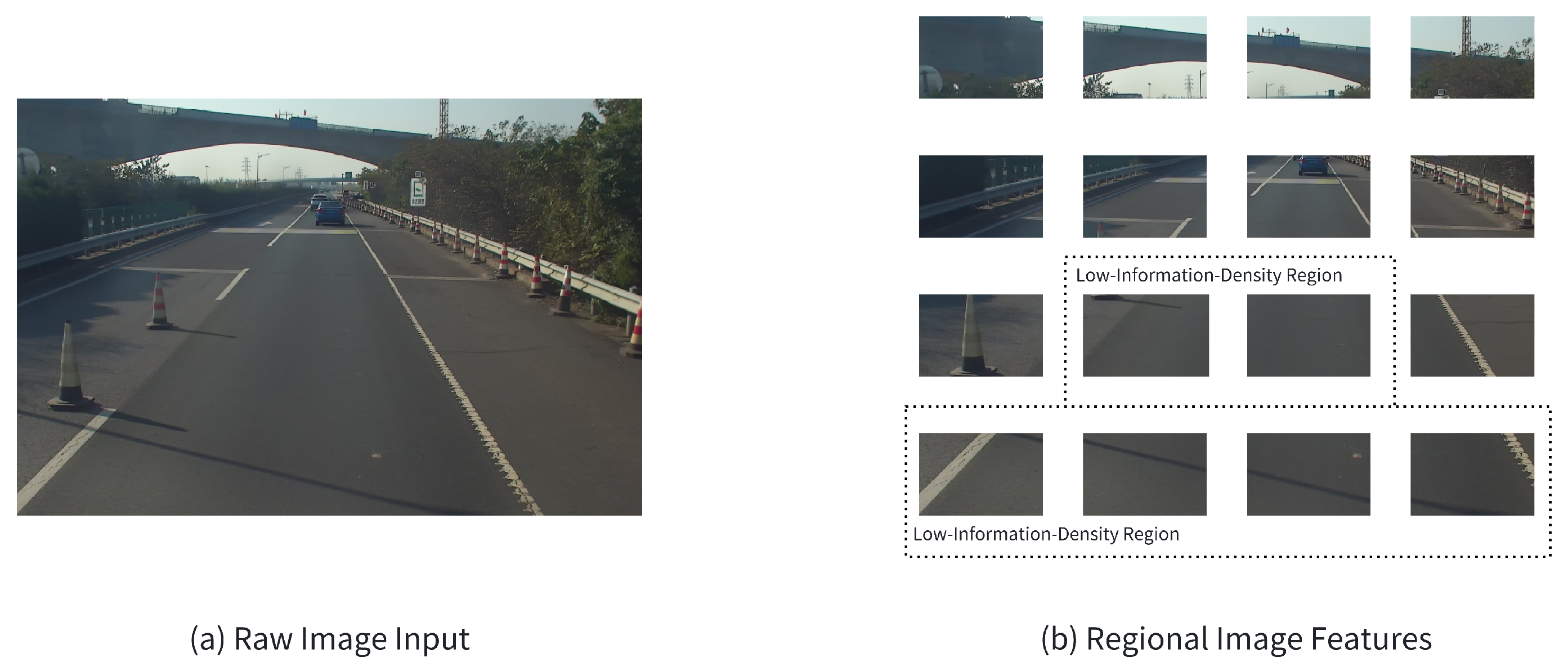
To address this limitation, we design a token differentiation scoring method based on semantic similarity between visual tokens. To maximize information retention, we prioritize retaining tokens with significant differentiation within local regions and dynamically select different sparsity levels to adapt to regional characteristics, as illustrated in Figure 3, which shows the image region feature differentiation.

Each local feature block $X_i(i=1,2,\dots ,N)$ consists of different token $X_i\left[j\right]$. For each $X_i$, we compute the pairwise cosine similarity $s_{jk}^{\left(i\right)}$ of the j-th and k-th token within the feature block $X_i$ to obtain matrix $S^{\left(i\right)}$ as shown in Equation (7):

$$s_{jk}^{\left(i\right)}={\displaystyle \frac{X_i\left[j\right]·X_i\left[k\right]}{\parallel X_i\left[j\right]\parallel \parallel X_i\left[k\right]\parallel }}$$

(7)

Here, $X_i\left[j\right]$ and $X_i\left[k\right]$ represent the j-th token and the k-th token of the i-th feature block $X_i$, where $j,k=1,2,\dots ,M$ and $M=576$. $\parallel X_i\left[j\right]\parallel$ and $\parallel X_i\left[k\right]\parallel$ are the Euclidean norms of the j-th token and the k-th token, respectively, representing the magnitude of the vectors. The calculation involves normalization by their norms to obtain normalized similarity, eliminating the influence of different feature scales on similarity computation. A value of $s_{jk}^{\left(i\right)}\in S^{\left(i\right)}$ closer to 1 indicates higher semantic similarity between token j and k; closer to 0 indicates greater independence.

Subsequently, for each token j, we compute its average similarity with other tokens as shown in Equation (8):

$${\stackrel{-}{S}}_j^{\left(i\right)}={\displaystyle \frac{1}{M-1}}\sum _{k\ne j}{s}_{jk}^{\left(i\right)}$$

(8)

${\stackrel{-}{S}}_j^{\left(i\right)}$ represents the average similarity of token j with other tokens, used to measure the degree of similarity of this token within the entire feature block. A lower average similarity indicates greater differentiation of the token from other tokens and higher uniqueness.

We define the token differentiation score $D_j^{\left(i\right)}$ to calculate its differentiation proportion within the region as shown in Equation (9):

$$D_j^{\left(i\right)}=1-{\stackrel{-}{S}}_j$$

(9)

If $D_j^{\left(i\right)}$ is close to 0, it indicates that the token is highly similar to its surroundings; if $D_j^{\left(i\right)}$ is close to 1 (theoretical maximum), the token is highly unique. All the differentiation scores $D_j^{\left(i\right)}$ from block features $X_i$ compose the token differentiation vector $D^{\left(i\right)}$.

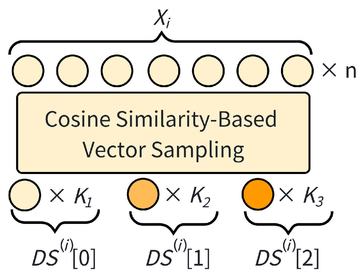
For each local feature $X_i$, we employ a Top-K approach to generate representations at different scales. The multi-scale representation is defined with different $K_s(s=0,1,2)$ values corresponding to sizes $\{n,{\displaystyle \frac{n}{4}},{\displaystyle \frac{n}{8}}\}$, where $n=M$ is the number of features within the local feature block. Through this processing pipeline, we generate three feature token sets at different resolutions: $D{S}^{\left(i\right)}\left[0\right]$ represents the feature vector obtained through the first type of down-sampling, $D{S}^{\left(i\right)}\left[1\right]$ corresponds to the feature vector produced by the second type of down-sampling, and $D{S}^{\left(i\right)}\left[2\right]$ is the feature vector generated by the third type of down-sampling. The overall process is shown in Equation (10):

$$D{S}^{\left(i\right)}\left[s\right]=\mathrm{TopK}(X_i,D^{\left(i\right)},K_s)$$

(10)

where, $\mathrm{TopK}(X_i,D^{\left(i\right)},K_s)$ ranks the tokens in $X_i$ by evaluating their differentiation scores $D^{\left(i\right)}$ to selects the top $K_s$ tokens, and returns a token subset $D{S}^{\left(i\right)}\left[s\right]$, which is a subset of $X_i$ composed of the top $K_s$ informative tokens. The process of our dynamic selection is as shown in Figure 4.

3.2.4. Dynamic Scale Selection

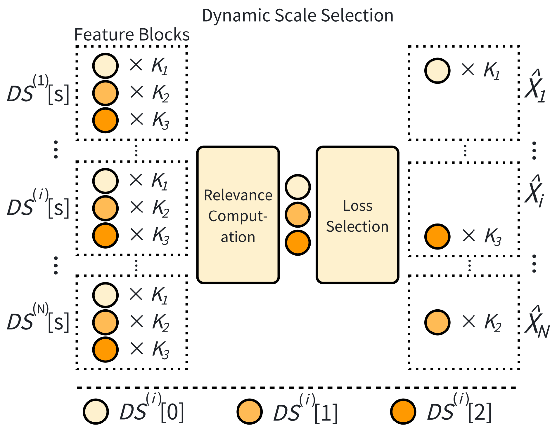
After completing similarity-based multiscale downsampling, the model faces a core challenge: how to adaptively select the most appropriate sampling scale for each local image region. To address this, we propose a dynamic scale-selection mechanism that leverages global contextual semantics to choose the visual representation with optimal information and contextual fit from multiple scale candidates, as illustrated in Figure 5.

First, for each scale candidate feature representation $D{S}^{\left(i\right)}\left[s\right]$ of region i for scale $s\in \{0,1,2\}$, we use global average pooling (AvgPool) to extract the regional semantic representation vector $h_i^s$ at each scale as shown in Equation (11):

$$h_i^s=\mathrm{AvgPool}\left(D{S}^{\left(i\right)}\left[s\right]\right)$$

(11)

This operation maps regional features at different sizes to a unified dimensional representation, facilitating subsequent alignment with global context. To determine whether local features at each scale align with the semantic objectives of the entire image, we introduce the whole-image encoding $v_g$ as global contextual information. For correlation computation, we flatten the spatial dimensions of $v_g$ to obtain $\mathrm{Flatten}\left(v_g\right)$. We then compute the correlation score between each local scale representation and the flattened global features. Specifically, the dot product between each candidate scale’s regional vector and the flattened global feature map produces a scale matching correlation matrix as shown in Equation (12):

$${\mathrm{Score}}_i^s=h_i^s\mathrm{Flatten}{\left(v_g\right)}^{\top }$$

(12)

where $h_i^s$ denotes the regional semantic representation vector of region i at scale s, and $\mathrm{Flatten}{\left(v_g\right)}^{\top }$ is the transpose of the spatially flattened global feature map $\mathrm{Flatten}\left(v_g\right)$.

We then flatten and compress this score matrix through a fully connected neural network layer denoted as $FC(·)$, mapping it to a scalar that represents the fit between this scale and the global semantics, as shown in Equation (13):

$$z_i^s=\mathrm{FC}\left(\mathrm{Flatten}\left({\mathrm{Score}}_i^s\right)\right)$$

(13)

We apply softmax processing to the scale score $z_i^s$ to obtain the selection probability $P_i\left(s\right)$ for each scale, as shown in Equation (14). Specifically, all scale-wise scores are aggregated into a vector $Z_i=(z_i^1,z_i^2,\dots ,z_i^S)$, where each $z_i^s$ represents the matching score of scale s. The softmax function is then applied over $Z_i$ to produce a normalized probability distribution across all scales:

$$P_i\left(s\right)=\mathrm{Softmax}\left(z_i^s\right)$$

(14)

where $\mathrm{Softmax}\left(z_i^s\right)$ denotes the s-th component of the resulting probability vector, corresponding to the selection probability of scale s. This probability distribution reflects the adaptation priority of each scale in the current context.

During training, to encourage the model to fully explore different scales and avoid premature convergence to a fixed scale, we adopt a probability-weighted fusion strategy as shown in Equation (15):

$${\hat{X}}_i=\sum _{s=0}^{S-1}{P}_i\left(s\right)·DS\left[s\right]\left(X_i\right)$$

(15)

That is, the sampling results of the $S(=3)$ scales are fused according to their probabilities to serve as the final visual representation of the region.

During inference, we employ a maximum probability selection strategy as shown in Equation (16) to improve computational efficiency and model determinism:

$${\hat{X}}_i=DS\left[\arg \max \left(Z_i\right)\right]\left(X_i\right)$$

(16)

That is, we directly select the features corresponding to the scale with the highest probability as the final representation of the region.

3.2.5. Loss Function Design

To prevent the selector from always choosing a fixed pooling scale, the model incorporates a certain degree of randomness and introduces a balance loss to encourage the selector to explore multiple pooling scales during training. This helps prevent the model from consistently selecting one fixed scale during training, ensuring that the selector can make more uniform choices across different pooling scales. Specifically, the balance loss constrains the selection probability of each pooling scale, preventing excessive bias toward any particular option. The balance loss formula is shown in Equation (17):

$${\mathcal{L}}_{\mathrm{balance}}=\alpha ·\sum _{s=0}^{S-1}{f}_s·\left({\displaystyle \frac{1}{N}}\sum _{i=1}^N{p}_i\left(s\right)\right)$$

(17)

where $\alpha$ is a hyperparameter determined via ablation experiments and s represents the index of the scales, with 3 candidate scales in total and $S=3$.

The $f_s$ is the frequency at which the s-th pooling scale is selected, as shown in Equation (18):

$$f_s={\displaystyle \frac{1}{N}}\sum _{i=1}^{N}1[\arg \max \left(q_i\right)=s]$$

(18)

where $\arg \max \left(q_i\right)$ represents the index of the scale with the highest probability among the S candidate scales for the i-th feature block.

The $p_i\left(s\right)$ is the softmax probability of scale s for the i-th feature block; as shown in Equation (19). N is the total number of feature blocks.

$$p_i\left(s\right)={\displaystyle \frac{1}{N}}\sum _{i=1}^N\mathrm{Softmax}\left(z_i^s\right)$$

(19)

3.2.6. Cross-Modal Fusion

In the vision-language model, the LLM primarily handles multimodal feature fusion and text generation. To achieve effective alignment between visual features and the language model, an embedding placeholder replacement mechanism is adopted to seamlessly integrate the visual vectors output by the image encoder into the input sequence of the LLM [21].

Specifically, the input of the VLM remains in the form of a natural language text, where a special visual placeholder (e.g., $\langle image\rangle$) is predefined to indicate the position of image information within the sequence. The language model first tokenizes the text input and converts each token into an embedding through the embedding layer. According to the output of the CLIP image encoder, each image is encoded into N visual tokens with length 768 [20]. Therefore, we employ N consecutive placeholder characters (e.g., @) to reserve the corresponding embedding slots for the image tokens, ensuring that the placeholder embedding dimension is consistent with the CLIP output.

After text embedding is completed, the token sequence generated by the image encoder is projected into the embedding space of the language model through a visual projector. These projected visual tokens then replace the embeddings of the predefined placeholders within the input sequence. The final multimodal input sequence can be expressed as:

$$\begin{array}{c}\hfill \mathrm{Input}=[\underset{\mathrm{Text}\mathrm{Token}}{\underbrace{{\mathrm{Token}}_1,{\mathrm{Token}}_2,\dots ,{\mathrm{Token}}_k}},\underset{\mathrm{Vision}\mathrm{Tokens}\mathrm{of}\mathrm{Block}1}{\underbrace{{\mathrm{VisionToken}}_{11},\dots ,{\mathrm{VisionToken}}_{1N}}},\\ \hfill \dots ,\underset{\mathrm{Vision}\mathrm{Tokens}\mathrm{of}\mathrm{Block}\mathrm{i}}{\underbrace{{\mathrm{VisionToken}}_{i1},\dots ,{\mathrm{VisionToken}}_{iN}}},\dots ]\end{array}$$

(20)

After replacing the visual placeholder, the subsequent processing flow of the language model is completely consistent with pure text input, still using an autoregressive generation method to gradually predict the next token until outputting a complete answer or generating a termination (such as EOS). This input format allows visual information to be naturally embedded in the language model context, neither disrupting the original language model structure nor efficiently achieving multimodal fusion.

3.2.7. Two Stage Training: Pretraining and Instruction Fine-Tuning

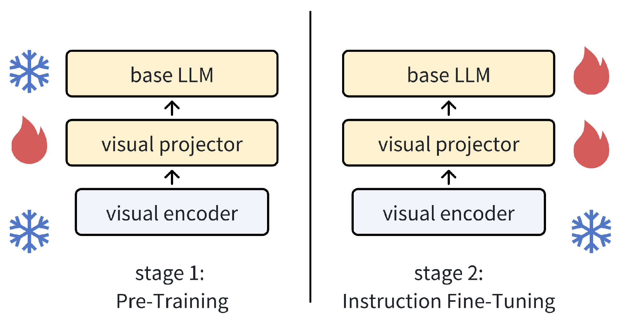
The training procedure follows a two-stage pipeline, as illustrated in Figure 6. The pretraining stage aims to align the visual and linguistic embedding spaces. A large-scale image-text pair corpus is used to train the projector that maps visual features into the language model’s embedding space. During this stage, both the vision encoder and the language model are frozen, and only the projector parameters are updated during training on the CC595K [21] dataset. This design mitigates overfitting risks while reducing computational cost.

The instruction fine-tuning stage further enhances multimodal instruction-following ability by training on multimodal instruction datasets LLaVA-Instruct-150K [22]. In this phase, both the projector and the language model parameters are updated in an end-to-end manner, while the vision encoder remains frozen to prevent overfitting of visual features.

The two-stage training on generalization-oriented datasets enhances the representation and reasoning capabilities of our DL-VLM, establishing a solid foundation for subsequent domain-specific fine-tuning and knowledge augmentation in bridge SHM tasks.

3.3. Domain-Specific Fine-Tuning Based on Bridge-SHM Dataset

To efficiently adapt the model introduced in Section 3.2 to the bridge construction domain, we adopts a hybrid fine-tuning strategy. The workflow of domain-specific fine-tuning is illustrated in Figure 1 Phase II. During the training, the parameters of the vision encoder are frozen to preserve its feature extraction capability for visual inputs, while the visual projector is allowed to update so that the alignment between visual and textual representations can be optimized. Meanwhile, LLM is fine-tuned using the parameter-efficient method LoRA (Low-Rank Adaptation of Large Language Models), which enhances the model’s ability to process language information while mitigating the risk of overfitting. During training, the pretrained model weights remain fixed, and only the low-rank matrices $\mathbf{A}$ and $\mathbf{B}$ are updated. Matrix $\mathbf{A}$ is initialized with a Gaussian distribution, whereas $\mathbf{B}$ is initialized as a zero matrix. The dimensions of the model inputs and outputs remain unchanged, and the outputs of the low-rank branch are added to the pretrained model parameters.

During fine-tuning, the model is trained on structured image–dialogue pairs from the Bridge-SHM dataset, where each sample consists of an image and a multi-turn conversation covering typical engineering scenarios such as bridge construction stages, defect identification, and structural analysis. Training follows the standard Causal Language Modeling (CLM) objective, computing the loss on each “gpt” response segment. Images are first processed by the frozen vision encoder, and the resulting embeddings are fed into the language model together with the dialogue history for contextual modeling.

3.4. Knowledge Augmentation

3.4.1. Semantic Representation of Knowledge Triples

To enable large language models to effectively utilize structured knowledge and improve semantic reasoning in the diagnostic workflow, we employ a template-based method that transforms symbolic knowledge graph triples into natural language descriptions.

Knowledge graphs typically store information in the form of triples, where each triple consists of three components: a head entity, a relation, and a tail entity. For each triple $p=(h,r,t)$ in the knowledge graph, where h is the head entity, r is the relation, and t is the tail entity, the system selects the template $r_p$ corresponding to relation r. The head entity h, template $r_p$, and tail entity t are then concatenated linearly to form a natural language sentence d. Ultimately, the knowledge graph G is transformed into a text corpus D composed of these sentences.

To further enhance retrieval efficiency, each bridge in the knowledge graph is assigned a unique identifier, referred to as the “bridge index.” This identifier serves as the core reference used to locate and unify all triples associated with a specific bridge across the graph. Once a query is mapped to a bridge index, the system can directly retrieve information from that bridge’s dedicated text corpus, thereby narrowing the search space and improving both retrieval accuracy and relevance.

For the triple corpus constructed for the bridge construction domain, we designate existing ontology schema classes (e.g., BridgeSuperstructure, ConstructionProgress, SubScenarios) as entity sets. These classes are mapped using domain-specific terminology from bridge engineering. Common linguistic expressions in bridge construction and maintenance are summarized, distilled into their underlying semantic logic, and subsequently mapped into triples. Examples of these mappings are shown in

Table 1. Examples of Triple-to-Sentence Mapping.

Head Entity	Relation Type	Tail Entity	Mapped Sentence Pattern
Pier 4#0	usedOccurred	Scouring and Erosion	Scouring and erosion were observed at Pier 4#0
Standard Column 0#	connectTo	Pier 1#0	Standard Column 0# is connected to Pier 1#0
Arch Rib Construction	nextStep	Column Construction	After arch rib construction is completed, column construction will begin
Bearing Aging	causedBy	Thermal Stress	Bearing aging may be caused by thermal stress
Deck Cracks	requires	Crack Sealing	Crack sealing treatment is required for deck cracks
Bearing Slip	recordedIn	2021 Inspection Report	The bearing slip phenomenon was recorded in the 2021 inspection report

.

3.4.2. Retrieval-Augmented Workflow

This module adopts a DPR-based retrieval-augmented generation framework, combined with a graph-structured knowledge base, to achieve fine-grained and structurally aligned knowledge retrieval and integration. The overall workflow is shown in Figure 1 Phase III.

For each bridge, a dedicated knowledge repository is constructed, containing multiple structured background knowledge triples. Each triple or document fragment is encoded into a dense vector using a DPR encoder and stored in a vector database. Similarly, the input query is encoded into a vector, denoted as q. The system then computes the cosine similarity between the query vector q and the vector representation d of each triple or document, as shown in Equation (21).

$$\mathrm{cosine}\mathrm{similarity}(q,d)={\displaystyle \frac{q·d}{\parallel q\parallel \parallel d\parallel }}$$

(21)

The vectors q and d represent the encoded query and triple/document vectors, respectively. Based on the similarity scores, the system retrieves the top-k most relevant triples, denoted as ${\mathcal{T}}_{\mathrm{retrieved}}$.

The system then extracts all entities appearing in the initial top-k triples and treats them as starting points for subgraph expansion. Cypher queries are constructed to retrieve triples directly connected to these entities or within two hops of them. Using the entities present in the initially retrieved triples, the system constructs a richer, locally closed subgraph, potentially incorporating indirectly related entities for improved reasoning coverage. The full process is shown in Algorithm 1.

Algorithm 1 Graph Expansion via Cypher Queries.

Require: top-k triples $\mathcal{T}=\left\{(h_i,r_i,t_i)\right\}$, Neo4j client neo4j_client, max expansion N, hop H Ensure: Expanded triple set ${\mathcal{T}}_{\mathrm{expanded}}$ 1: Initialize entity set $\mathcal{E}\leftarrow ⌀$ 2: for each $(h,r,t)\in \mathcal{T}$ do 3:     $\mathcal{E}\leftarrow \mathcal{E}\cup \{h,t\}$ 4: end for 5: entity_list ← list ($\mathcal{E}$) 6: if $H=1$ then 7:     Construct 1-hop Cypher query: MATCH (e)-[r]->(n) WHERE e.name IN entity_list RETURN e.name AS head, type(r) AS relation, n.name AS tail LIMIT N; 8: else 9:     Construct 2-hop Cypher query: MATCH (e)-[r1]->(m)-[r2]->(n) WHERE e.name IN entity_list RETURN e.name AS head, type(r1) AS rel1, m.name AS mid, type(r2) AS rel2, n.name AS tail LIMIT N; 10: end if 11: Run Cypher query, get result ← neo4j_client.run(query) 12: Initialize expanded triple set ${\mathcal{T}}_{\mathrm{expanded}}\leftarrow ⌀$ 13: for each record in result do 14:    if $H=1$ then 15:         $\mathcal{T}\leftarrow {\mathcal{T}}_{\mathrm{expanded}}\cup \left\{(\mathrm{record}.\mathrm{head},\mathrm{record}.\mathrm{relation},\mathrm{record}.\mathrm{tail})\right\}$ 16:    else if $H=2$ then 17:         Convert 2-hop path to triples and add to ${\mathcal{T}}_{\mathrm{expanded}}$ 18:    end if 19: end for 20: return  ${\mathcal{T}}_{\mathrm{expanded}}$

After semantic retrieval and graph expansion, the system obtains the union of two triple sets: the top-k triples from DPR retrieval, ${\mathcal{T}}_{\mathrm{retrieved}}$, and the n triples expanded from the graph database, ${\mathcal{T}}_{\mathrm{expanded}}$. These are merged into a unified candidate set, as shown in Equation (22).

$${\mathcal{T}}_{\mathrm{cand}}={\mathcal{T}}_{\mathrm{retrieved}}\cup {\mathcal{T}}_{\mathrm{expanded}}$$

(22)

To further improve input quality, a Cross-Encoder-based reranker is used to fine-rank the candidate triples. The query Q and each triple $T_i$ are concatenated into an input pair $[Q,T_i]$, which is fed into the Cross-Encoder to produce a relevance score $s_i$, as shown in Equation (23).

$$s_i=CrossEncoder(Q,T_i)$$

(23)

The triples are ranked in descending order of their scores, and the top-k most relevant triples are selected as the final background knowledge for the language model. This filtering step removes redundant or weakly relevant knowledge, ensuring a concise and context-specific input that improves the accuracy and interpretability of the model’s generated answers.

Finally, the selected triples are transformed into natural language using the semantic representation method introduced in Section 3.4.1. These semanticized triples are concatenated with the original user query to form the final input context for downstream reasoning and generation.

4. Computational Experiments

4.1. Data and Model Training

4.1.1. Dataset for Pretraining and Instruction Fine-Tuning

In Phase I, to equip DL-VLM with strong general visual–text understanding and robust multimodal reasoning capability, we adopt two types of datasets for the model’s general-purpose training: (a) a large-scale image–text corpus for multimodal pretraining, and (b) an instruction-oriented multimodal dataset for alignment tuning.

(1) CC595K  [21]. During the pretraining stage of Phase I, we employ the CC595K dataset, a widely used subset of the Conceptual Captions collection consisting of high-quality image–caption pairs. The dataset covers diverse natural image domains and rich textual descriptions, enabling the visual encoder and multimodal fusion layers to learn robust visual grounding, object–scene understanding, and cross-modal semantic alignment. This pretraining stage provides DL-VLM with strong generalization ability prior to any domain adaptation.

(2) LLaVA-Instruct-150K [22]. To further enhance multimodal reasoning and instruction-following ability, during the instruction fine-tuning stage of Phase I, we adopt the LLaVA-Instruct-150K dataset, which contains image–instruction-response triplets derived from GPT-generated guidance. The dataset includes detailed reasoning chains, conversational instructions, and task-oriented visual queries. By fine-tuning on these instruction-style samples, DL-VLM learns to perform step-by-step reasoning, produce coherent explanations, and follow human-like multimodal instructions. This stage effectively aligns the model with high-level reasoning behaviors required for downstream applications.

4.1.2. Evaluation Datasets

To evaluate the performance of the generalization capability of DL-VLM in Phase I, we adopt five widely used open-source benchmarks in the vision-language modeling domain.

(1) GQA [37]: The GQA dataset is constructed based on three core components: scene graphs, questions, and images. In addition to image content, it provides rich spatial information and object-level attributes, offering structured support for visual understanding. The questions are designed to systematically evaluate models on complex scene understanding, logical reasoning, and multi-step inference.

(2) ScienceQA (SQA) [38]: ScienceQA covers multiple disciplines, including natural sciences, linguistics, and social sciences, exhibiting strong interdisciplinary characteristics. Questions are organized hierarchically into 26 topics, 127 categories, and 379 specific skills, forming a rigorous and diverse evaluation platform. This multi-level structure facilitates comprehensive assessment of multimodal reasoning, information integration, and interpretability, while promoting the advancement of multimodal models in complex real-world contexts.

(3) TextVQA (VQA) [39]: TextVQA focuses on evaluating the ability to extract and understand textual information embedded in images. It emphasizes deep fusion of visual and textual modalities, requiring models to not only read natural scene text (e.g., signs, screens, labels) but also perform semantic reasoning for accurate answers. This benchmark is particularly demanding on OCR accuracy, text localization, and cross-modal reasoning, serving as a key standard for assessing text-aware VQA capabilities.

(4) POPE [40]: The POPE benchmark is specifically designed to evaluate object hallucination in multimodal models. It formulates binary existence questions about objects within an image, enabling quantitative analysis of models’ tendency to generate fictitious content.

(5) MMB [41]: The MMB platform provides a comprehensive evaluation of large vision-language models across multiple subtasks, including image-text understanding, matching, commonsense reasoning, OCR, and visual reasoning. It is widely regarded as a benchmark for assessing the overall capabilities of state-of-the-art vision-language models such as GPT-4V and Gemini.

4.1.3. Bridge-SHM Dataset

To comprehensively evaluate the performance of our model in Phase II and Phase III, we construct a bridge-related dataset derived from private bridge inspection datasets. These datasets collectively form the Bridge-SHM dataset, which serves as the foundation of the proposed vision–language modeling framework.

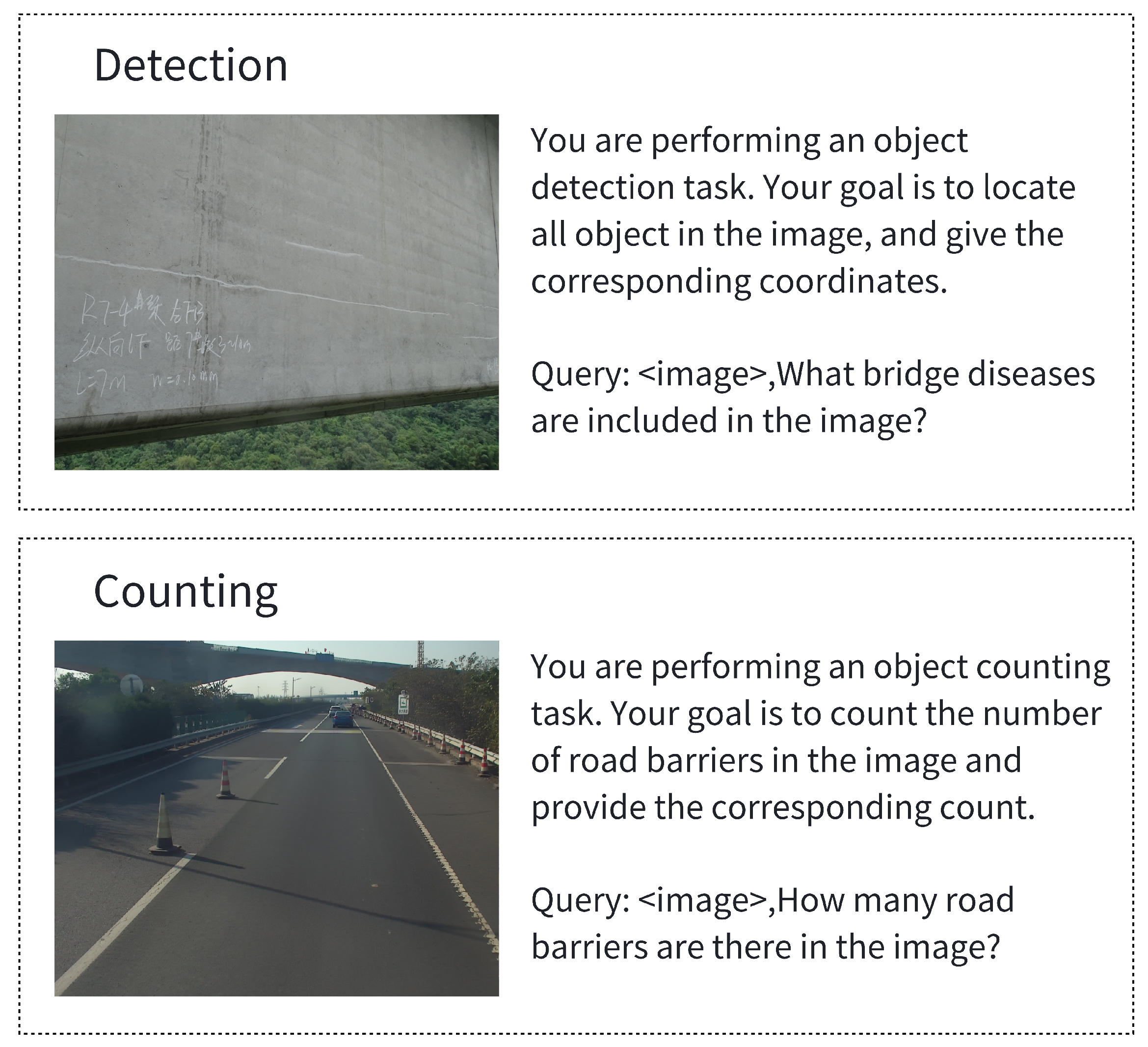
We first develop a domain-specific image dataset that captures representative visual conditions in bridge engineering. As summarized in

Table 2. Composition of the Bridge-SHM Dataset.

Category	Description	Size
Bridge construction scenes	Various construction scenarios	7289
Bridge surface defects	Eight defect types in RC structures	3658
Structural component images	Piers, girders, bearings, connectors	2642

, the dataset contains 13,589 images categorized into three major groups: bridge construction scenes, bridge surface defects, and critical structural components. This dataset supports downstream tasks such as structural inspection, defect recognition, and condition assessment. Examples of these scenes are illustrated in Figure 7.

The construction-scene subset includes operations such as concrete pouring, rebar tying, and formwork installation, as well as safety-related contexts such as helmet use and protective procedures. The surface-defect subset focuses on reinforced-concrete structures and includes major defect categories such as corrosion, cracking, degradation, voids, moisture intrusion, pavement deterioration, and shrinkage cracks. The structural-component subset contains images of key elements including piers, girders, bearings, and steel connectors.

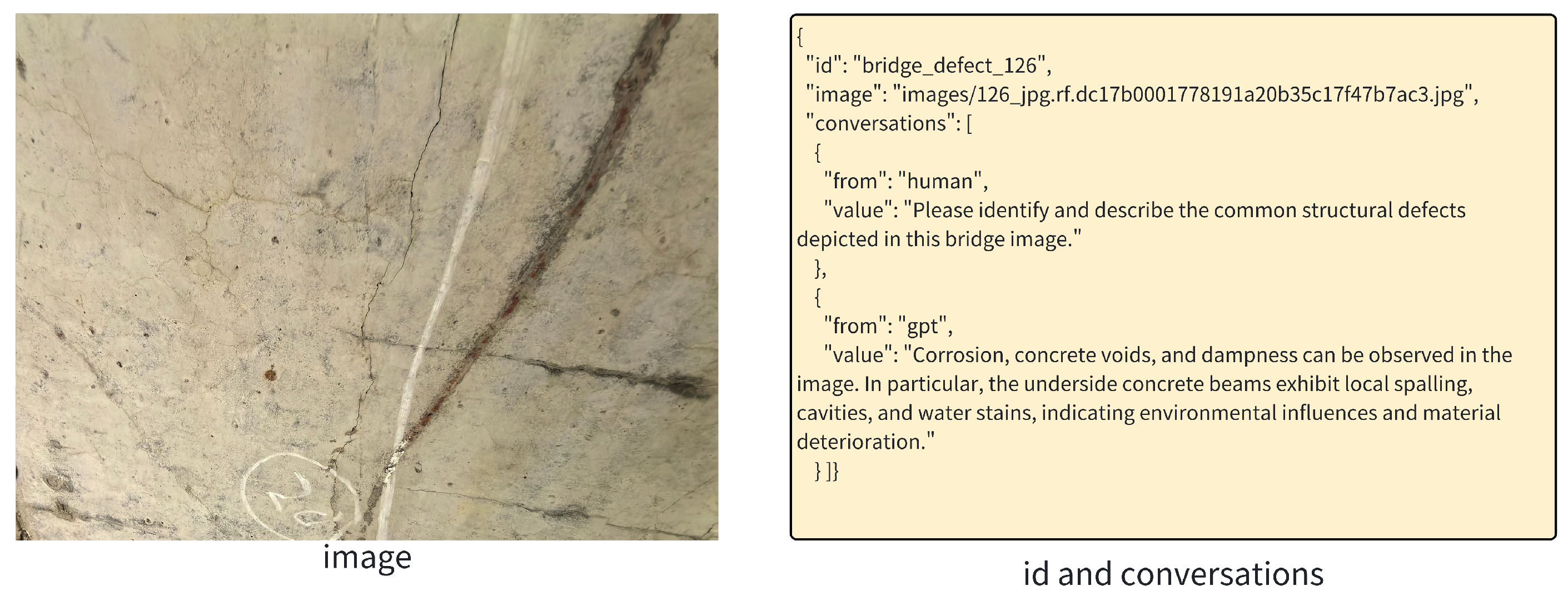
Following the data-format specification of the LLaVA dataset, we construct a structured vision–language alignment corpus in which each training sample consists of an image path and a multi-turn dialogue. All data are stored in JSON format with fields including id, image, and conversations. An illustrative example is provided in Figure 8. Compared with traditional single-turn annotations, this multi-turn alignment format better reflects real-world SHM workflows, where iterative clarification and contextual reasoning are essential. Bridge engineering terminology and task-specific descriptions are carefully incorporated to ensure professional accuracy. Part of the annotation data is generated with assistance from LLMs and is further refined through manual proofreading, improving annotation efficiency while maintaining high-quality and domain-consistent supervision.

In vision tasks, data augmentation is widely used—particularly in object detection and image classification—to enhance robustness against variations in viewpoint, lighting, scale, and noise. However, for VLM training, augmentation must be applied with caution. Since the objective of VLMs is to learn meaningful alignment between visual content and natural-language expressions, augmentations that substantially alter scene structure, color distribution, or spatial layout may disrupt image–text semantic consistency.

For instance, in bridge construction scenes, horizontally flipping an image may contradict textual descriptions such as “the crane is on the left side of the bridge,” leading to misalignment and degraded model performance. Similarly, aggressive cropping, occlusion, excessive brightness reduction, or strong color perturbations may remove or distort key semantic elements, making the image inconsistent with its associated text.

For these reasons, we adopt only mild brightness perturbation—an augmentation that preserves spatial semantics while providing moderate visual diversity—to enhance robustness within the Bridge-SHM dataset. The augmentation process is illustrated in Figure 9.

4.2. Experimental Setup

All experiments are conducted on a server equipped with four NVIDIA Tesla V100 GPUs (24 GB memory each). Tesla V100, based on the Volta architecture, provides 5120 CUDA cores and 640 Tensor cores, enabling highly parallelized computations well-suited for deep learning tasks. Its 24 GB high-bandwidth memory (HBM2) ensures efficient handling of large-scale training data. The software environment consists of Ubuntu 20.04 LTS with CUDA 11.8 and cuDNN 8.2.1. PyTorch 2.0.1 and Python 3.10 are used for model development. To further optimize training efficiency, mixed-precision training is enabled, leveraging Tensor cores for accelerated computation while reducing memory overhead.

Specifically, pretraining is conducted on a curated subset of the CC595K [21] dataset with a batch size of 64 and an initial learning rate of $1\times {10}^{-3}$. Instruction fine-tuning is then performed on the LLaVA-Instruct-150K [22] dataset with a batch size of 32 and a learning rate of $4\times {10}^{-5}$. AdamW optimizer is adopted with weight decay set to 0, momentum parameters ${\beta }_1=0.9$, ${\beta }_2=0.999$, and $ϵ=1\times {10}^{-8}$. During fine-tuning, all parameters of the language model are updated.

In our domain-specific fine-tuning and knowledge augmentation module, the knowledge graph is managed and queried using Neo4j 5.12 [42] deployed on a local server. For dense retrieval, we adopt Facebook AI Research’s open-source DPR models [30], namely the DPR-Question Encoder and the DPR-Context Encoder, which are used to encode the queries and candidate knowledge contexts, respectively. Vector storage and similarity search are implemented using Faiss, enabling efficient large-scale vector indexing and retrieval. For semantic reranking, we adopt an MS MARCO–trained MiniLM Cross-Encoder [31] to refine the semantic relevance between the query and the retrieved candidate triplets. All computations involved in knowledge retrieval, vector indexing, and reranking are executed under CUDA 11.8 to ensure efficient multi-GPU parallelism. In addition, for all model training stages in our framework, the corresponding datasets are consistently divided into training, validation, and test sets following an 8:1:1 ratio to ensure a stable and rigorous evaluation protocol.

4.3. Evaluation Metrics

4.3.1. Evaluation Metrics for Generalized DL-VLM

For the GQA visual reasoning benchmark, each sample is provided with a single ground-truth answer. Therefore, the evaluation metric follows the standard Top-1 accuracy protocol, defined as:

$${\mathrm{Acc}}_{\mathrm{GQA}}=\left\{\begin{array}{cc}1,\hfill & \mathrm{if}\hat{y}=y,\hfill \\ 0,\hfill & \mathrm{otherwise}.\hfill \end{array}\right.$$

(24)

Similar to GQA, ScienceQA also provides a single correct answer for each question. Thus, Top-1 Exact Match Accuracy is used, defined as:

$${\mathrm{Acc}}_{\mathrm{SQA}}=\left\{\begin{array}{cc}1,\hfill & \mathrm{if}\hat{y}=y,\hfill \\ 0,\hfill & \mathrm{otherwise}.\hfill \end{array}\right.$$

(25)

The VQA-v2 benchmark adopts a consensus-based scoring rule, where an answer is considered correct if it matches the majority of annotators. The accuracy for each sample is computed as:

$${\mathrm{Acc}}_{\mathrm{VQA}}=min\left({\displaystyle \frac{1}{3}}\sum _{j=1}^{10}\mathbf{1}(\hat{y}=y_j),1\right),$$

(26)

where $y_j$ denotes the j-th human annotator’s answer.

The POPE benchmark evaluates object hallucination by verifying whether the predicted object exists in the ground-truth object set. The hallucination rate is defined as:

$$\mathrm{Hallucination}=\left\{\begin{array}{cc}1,\hfill & \mathrm{if}\hat{o}\notin O,\hfill \\ 0,\hfill & \mathrm{otherwise},\hfill \end{array}\right.$$

(27)

where O denotes the set of objects actually present in the image.

MMBench evaluates multi-level perception and reasoning ability using a scoring protocol based on question difficulty. The final score is computed as:

$${\mathrm{Score}}_{\mathrm{MMB}}={\displaystyle \frac{1}{M}}\sum _{k=1}^M{s}_k,$$

(28)

where $s_k$ denotes the correctness score for the k-th question.

4.3.2. Evaluation Metrics for Domain-Specific Fine-Tuning

For the domain-specific fine-tuning visual question answering (VQA) task, we employs the standard accuracy evaluation protocol commonly used in VQA benchmarks [39] as the primary performance metric. Each test sample consists of an image, a question, and multiple candidate answers, and the model is required to select the most appropriate one.

For the bridge engineering VQA test set constructed in this paper, each question is designed with a single ground-truth answer. Therefore, we adopt Top-1 Exact Match Accuracy as the evaluation metric, as shown in Equation (29):

$$\mathrm{Accuracy}=\left\{\begin{array}{cc}1,\hfill & \mathrm{if}\mathrm{predicted}\mathrm{option}=\mathrm{correct}\mathrm{answer},\hfill \\ 0,\hfill & \mathrm{otherwise}.\hfill \end{array}\right.$$

(29)

4.3.3. Evaluation Metrics for Knowledge Augmentation

In knowledge augmentation, we utilize the RetrieverEvaluator interface provided by the LlamaIndex framework to evaluate retrieval performance. By simply supplying the evaluation samples, vector database, and retrieval model, the system automatically performs the evaluation procedure and outputs key performance indicators such as Hit Rate and MRR.

Hit Rate measures the proportion of returned results that are judged to be relevant or useful to the user. It reflects the system’s ability to provide effective information and serves as one of the most important indicators of retrieval quality. The calculation is shown in Equation (30):

$$\mathrm{Hit}\mathrm{Rate}={\displaystyle \frac{\mathrm{Number}\mathrm{of}\mathrm{Hits}}{\mathrm{Total}\mathrm{Number}\mathrm{of}\mathrm{Queries}}}$$

(30)

Here, the number of hits refers to the count of retrieved items that are considered relevant or useful, while the total number of queries denotes the total number of retrieval requests issued by the user. Hit Rate is computed as the ratio of these two values and reflects the system’s ability to satisfy user information needs.

Mean Reciprocal Rank (MRR) measures the position of the most relevant item in the ranked retrieval results. As shown in Equation (31), it is calculated by taking the reciprocal of the rank of the most relevant result for each query and then averaging across all queries. This metric emphasizes how early the most relevant result appears in the returned list—higher MRR values indicate better retrieval performance.

$$\mathrm{MRR}={\displaystyle \frac{1}{Q}}\sum _{i=1}^Q{\displaystyle \frac{1}{{\mathrm{rank}}_i}}$$

(31)

In this equation, Q represents the total number of queries, and ${\mathrm{rank}}_i$ denotes the ranking position of the most relevant result for the i-th query. The value of MRR ranges from 0 to 1, with 1 indicating that the most relevant result always appears at the top of the ranked list, and 0 indicating that relevant results never appear in the top positions. A higher MRR reflects better retrieval capability.

4.4. Experiment Results

4.4.1. Experiments on the General DL-VLM

(1) 

Comparison Studies

The proposed model demonstrates consistent advantages across different parameter scales. For small-parameter configurations, the model achieves varying degrees of improvement on multiple benchmark tests, indicating that it can effectively enhance performance even under resource-constrained settings. Such gains may stem from architectural optimizations, improved training strategies, or enhanced task-specific adaptability.

In experiments with large-parameter configurations, although the model does not significantly surpass competing methods on all benchmarks, its performance remains comparable to state-of-the-art models, showing that it retains strong competitiveness in high-complexity tasks. This suggests that the proposed method is not only suitable for small-scale models but also maintains stable performance in large-scale settings, further validating its generalization ability and robustness.

Table 3. Performance comparison of small-scale models across multiple benchmarks.

Method	LLM	SQA	VQA	GQA	MMB	POPE
MobileVLM 1.7B	MobileLLaMA 1.4B	54.7	41.5	56.1	53.2	84.5
MobileVLM V2	MobileLLaMA 1.4B	61.2	47.5	59.0	59.6	84.9
Xmodel-VLM	Xmodel-LM 1.1B	53.3	39.9	58.3	52.0	85.9
LLaVA-Phi	Phi2-2.7B	65.4	48.6	56.2	59.8	85.0
DeepSeek-VL	DeepSeek-1.3B	60.8	43.0	57.3	64.6	84.6
Ours	Phi2-2.7B	63.4	49.6	60.3	58.1	86.2

Experimental results on small-scale benchmarks.

and

Table 4. Performance comparison of large-scale models across multiple benchmarks.

Method	LLM	SQA	VQA	GQA	MMB
mPlugOwl3	Qwen-8B	-	69.0	61.0	77.6
Instruct-BLIP	Vicuna-7B	60.5	50.1	49.2	36.0
Qwen-VL	Qwen-7B	67.1	63.8	59.3	60.6
LLaVA-1.5	Vicuna-7B	66.8	58.2	62.0	62.0
Ours	Phi2-2.7B	63.4	49.6	60.3	58.1

Experimental results on 7B-scale benchmarks.

report comparative results across multiple benchmarks.

To further highlight the lightweight nature of our framework,

Table 5. Model size and resource comparison across different LLM backbones.

LLM Backbone	Parameters	Typical GPU Memory	Relative FLOPs
Phi2-2.7B (Ours)	2.7B	4–6 GB	1.0×
Vicuna-7B	7.0B	13–14 GB	2.4×
Qwen-7B	7.0B	14 GB	2.5×
Qwen-8B	8.0B	16 GB	3.0×

GPU memory and FLOPs values are estimated from official model documentation under FP16 inference: Phi-2 from Microsoft Research [43], Vicuna-7B from LMSYS, and Qwen models from the Qwen Technical Report [44].

provides a comparison of the model sizes and computational requirements of the LLM backbones used in the evaluated systems. Our method is built on the Phi2-2.7B backbone, which contains only 2.7B parameters and requires approximately 4–6 GB of GPU memory for FP16 inference. In contrast, the 7B–8B backbones used by large-scale baselines (e.g., Vicuna-7B, Qwen-7B, and Qwen-8B) require 13–16 GB of memory and incur 2.4–3.0× higher FLOPs per token.

This substantial reduction in model size directly contributes to lower computation cost, smaller memory footprint, and faster inference, enabling deployment in resource-constrained SHM scenarios. More importantly, the proposed dynamic down-sampling strategy further reduces latency by adaptively selecting an appropriate feature resolution for each input instead of processing all images at a fixed high resolution. By avoiding unnecessary high-resolution encoding when coarse-grained features are sufficient, the model significantly decreases ViT encoder workload while still preserving task-critical visual cues. Combined with the efficient projection design, this adaptive mechanism enables the model to achieve competitive or even superior performance compared to larger LLM-based frameworks, demonstrating that task-relevant visual information can be retained without relying on large model capacity.

The experimental results in Table 3 and Table 4 demonstrate that our method achieves a strong balance between accuracy and efficiency across different parameter scales. For small-scale backbones, our model attains competitive or leading performance on several key metrics: SQA = 63.4 (close to the best 65.4 of LLaVA-Phi), VQA = 49.6 (the best among listed small models), GQA = 60.3 (the best), MMB = 58.1 (near the top), and POPE = 86.2 (the best). These results indicate that the proposed dynamic multi-scale down-sampling and similarity-driven token selection effectively preserve task-relevant structural details, which is particularly reflected in the improvements on GQA and POPE. In comparison with MobileVLM and Xmodel-VLM variants, our method consistently improves VQA and GQA, demonstrating superior fine-grained visual–text alignment under constrained model capacity.

For 7B-scale comparisons, our framework remains competitive: although some very large baselines (e.g., mPlugOwl3 and Qwen-VL) achieve higher VQA or SQA scores (VQA up to 69.0 and SQA up to 67.1), our model (SQA = 63.4, VQA = 49.6, GQA = 60.3, MMB = 58.1) delivers comparable GQA and maintains solid performance across tasks while using a substantially smaller LLM. This highlights the efficiency advantages of our dynamic down-sampling strategy—the model is able to approach the reasoning capability of larger systems while requiring significantly fewer computational resources.

(2) 

Ablation Studies

To investigate the contributions of individual components, we conduct a series of ablation studies.

To investigate the impact of the visual projection mechanism on multimodal feature representation, we compare several projection architectures, including Linear, Q-Former, LDP, LDPv2, XDP, and our proposed dynamic down-sampling projection.

Table 6. Performance of different visual projection modules across multiple benchmarks.

Method	SQA	VQA	GQA	MMB
Linear	31.6	38.7	59.2	42.7
Q-Former	56.0	40.5	58.3	52.2
LDP	52.5	37.2	57.5	45.3
LDPv2	52.9	38.8	58.0	55.0
XDP	53.3	39.9	58.3	52.0
Ours	63.4	49.6	60.3	58.1

Experimental results comparing visual projection modules.

summarizes the performance across multiple benchmarks. The results indicate that selecting an appropriate projection module significantly enhances cross-modal feature complementarity, which directly improves downstream task performance. While Q-Former demonstrates higher accuracy in image-text matching tasks, our dynamic down-sampling projection consistently achieves superior results on SQA, VQA, GQA, and MMB, highlighting its effectiveness in preserving task-relevant visual information under resource-constrained settings.

Table 7. Performance of different backbone LLMs across multiple benchmarks.

Method	SQA	VQA	GQA	MMB
Qwen2.5-0.5B	49.3	38.7	55.2	42.7
TinyLlama-1.1B-Chat-v1.0	52.0	37.9	54.0	52.6
Gemma-2B-it	52.5	37.2	56.5	49.3
Phi2-2.7B	63.4	49.6	60.3	58.1

Experimental results comparing different backbone LLMs.

reports results using different backbone LLMs while keeping the vision encoder and projector fixed. Larger LLMs significantly improve overall performance, indicating that scaling the language model is an effective strategy when computational resources allow.

Table 8. Performance under different down-sampling scales.

Scales	SQA	VQA	GQA	MMB	POPE
$\{n,n/4,n/8\}$	63.4	49.6	60.3	58.1	86.8
$\{n,n/4,n/16\}$	62.8	48.4	59.2	57.8	85.2
$\{n,n/4,n/n\}$	52.6	38.9	54.8	51.5	83.0
$\{n,n/8,n/16\}$	63.7	49.1	57.4	57.5	86.7
All scales	64.8	51.5	60.1	57.4	85.7

Results show the performance of the model under different down-sampling scale settings across multiple benchmarks.

compares different scale configurations. The combination $\{n,n/4,n/8\}$ yields the best performance, especially on GQA, MMB and POPE, suggesting an effective balance between feature detail preservation and semantic abstraction.

Finally, we evaluate the impact of balancing loss weights (

Table 9. Impact of different loss weights on model performance across multiple benchmarks.

Weight	SQA	VQA	GQA	MMB
0.01	61.8	46.3	57.4	56.0
0.1	63.4	49.6	60.3	58.1
0.5	63.2	49.1	60.6	57.9

Results show the effect of varying the loss weight on the performance metrics of SQA, VQA, GQA, and MMB.

). Results show that very small weights fail to guide the sampling module effectively, while an intermediate setting 0.1 achieves the best trade-off, leading to improvements in VQA and GQA. Excessively large weights, however, interfere with the main task, limiting further gains.

The ablation experiments demonstrate the effectiveness and necessity of the proposed components. From Table 6, the dynamic down-sampling visual projection consistently outperforms alternative architectures, confirming its ability to preserve task-relevant visual features while enhancing cross-modal alignment. From Table 7, using a larger backbone LLM significantly improves overall performance, showing that language model capacity directly influences multimodal reasoning capability. From Table 8, the multi-scale down-sampling configuration $\{n,n/4,n/8\}$ achieves the best trade-off between preserving fine-grained structural details and abstracting semantic information, particularly benefiting GQA and POPE. Finally, from Table 9, tuning the loss weight is critical for guiding the dynamic sampling module: an intermediate value (0.1) provides the optimal balance, improving task performance without destabilizing the main objectives. Overall, these studies confirm that each individual component contributes to the efficiency and accuracy of the proposed framework, and their combined design enables strong performance under both small- and large-scale settings.

4.4.2. Experiments of Domain-Specialized Fine-Tuning

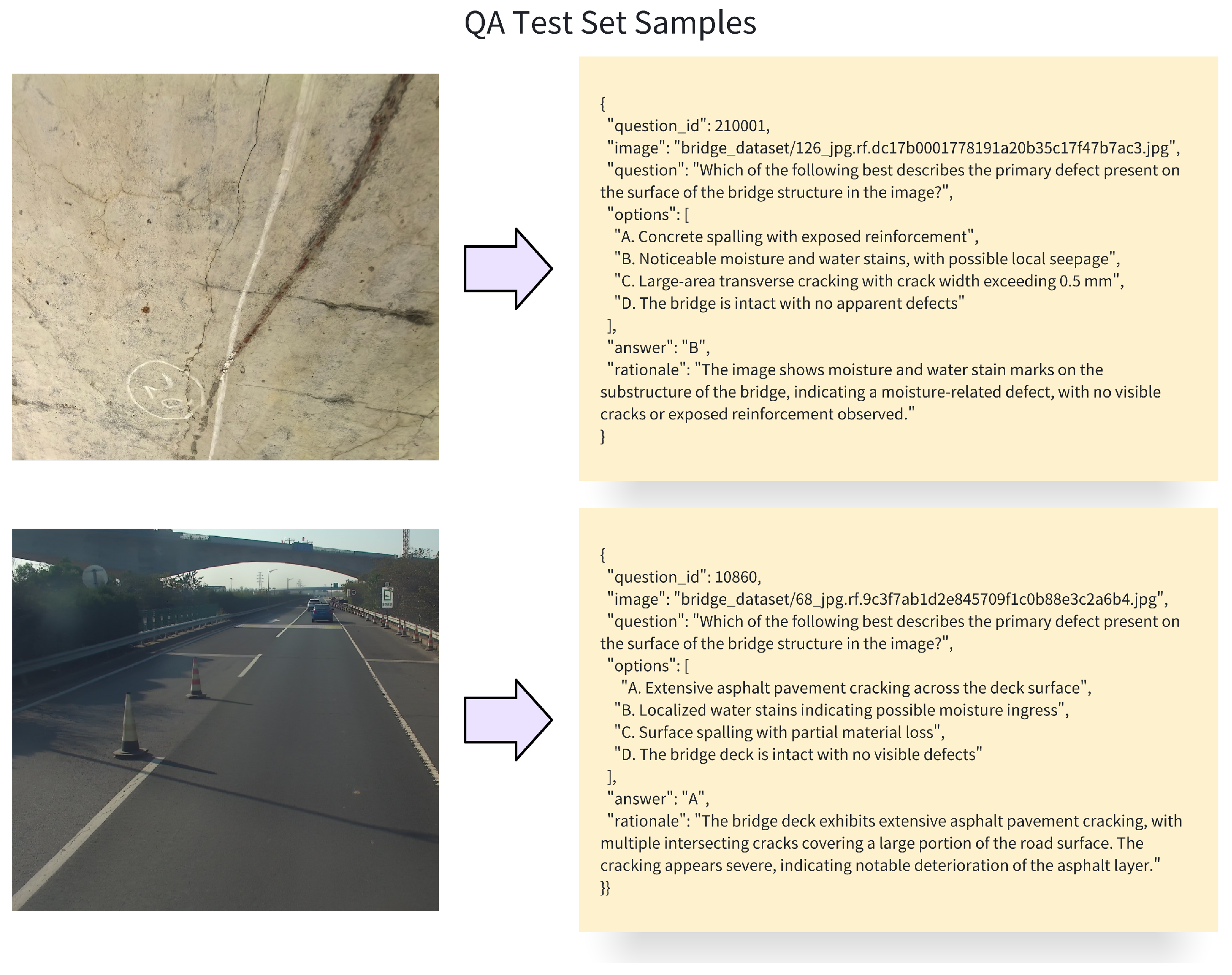
To verify the effectiveness of the fine-tuning strategies, we compare different visual projection mechanisms and parameter-efficient tuning methods on the test set. The results are summarized in

Table 10. Performance of different fine-tuning strategies on the test set.

Linear	DSFD	LoRA	QLoRA	Construction Site (%)	Bridge Defects (%)	Structural Inspection (%)
✓	×	×	×	49.5	37.6	36.9
×	✓	×	×	59.8	43.7	48.6
×	✓	✓	×	62.7	69.3	68.5
×	✓	×	✓	63.5	67.4	67.3

and examples of the QA task are presented in Figure 10. Here, Linear denotes a simple linear visual projector, DSFD refers to the dynamic sampling module proposed in Section 3.2, and LoRA and QLoRA represent the two parameter-efficient tuning techniques adopted in this module. QLoRA extends LoRA by incorporating quantization to further reduce storage and computational cost.

The results indicate that compared with the linear projector, the dynamic sampling module consistently improves performance across all three bridge-related tasks.

To further analyze the differences across image categories, we separately evaluate the model on construction-site images, surface-defect images, and structural-inspection images. The results show that the most significant improvements appear in surface defect and structural inspection images, where the average Top-1 accuracy increases from 43.7% and 48.6% before fine-tuning to 69.3% and 68.5% after fine-tuning.

Surface defect images often contain high–semantic-density patterns such as cracks, corrosion, and spalling. These details are difficult for general vision models to recognize, as such defects rarely appear in large-scale pretraining corpora.

In contrast, construction-site images already exhibit relatively good baseline accuracy prior to fine-tuning. This is likely because the vision encoders used in mainstream VLMs (e.g., CLIP in LLaVA) are pretrained on large-scale datasets such as LAION-400M, which contain many images with labels related to construction machinery, engineering scenes, and urban infrastructure. These images share semantic overlap with construction-site scenarios, enabling decent recognition without domain-specific fine-tuning.

However, bridge defect images (e.g., cracks, delamination, moisture, hollowing) appear very infrequently in open-source pretraining datasets and therefore belong to “rare semantic categories.” As a result, domain-specific fine-tuning yields substantial improvements for such images.

Finally, although QLoRA significantly reduces memory and computation, the quantization process may introduce accuracy loss—particularly for tasks requiring fine-grained semantic precision, such as defect recognition and structural analysis—resulting in slightly lower performance compared with LoRA.

4.4.3. Experiments on Knowledge Augmentation

(1)

Single-Vector Retrieval

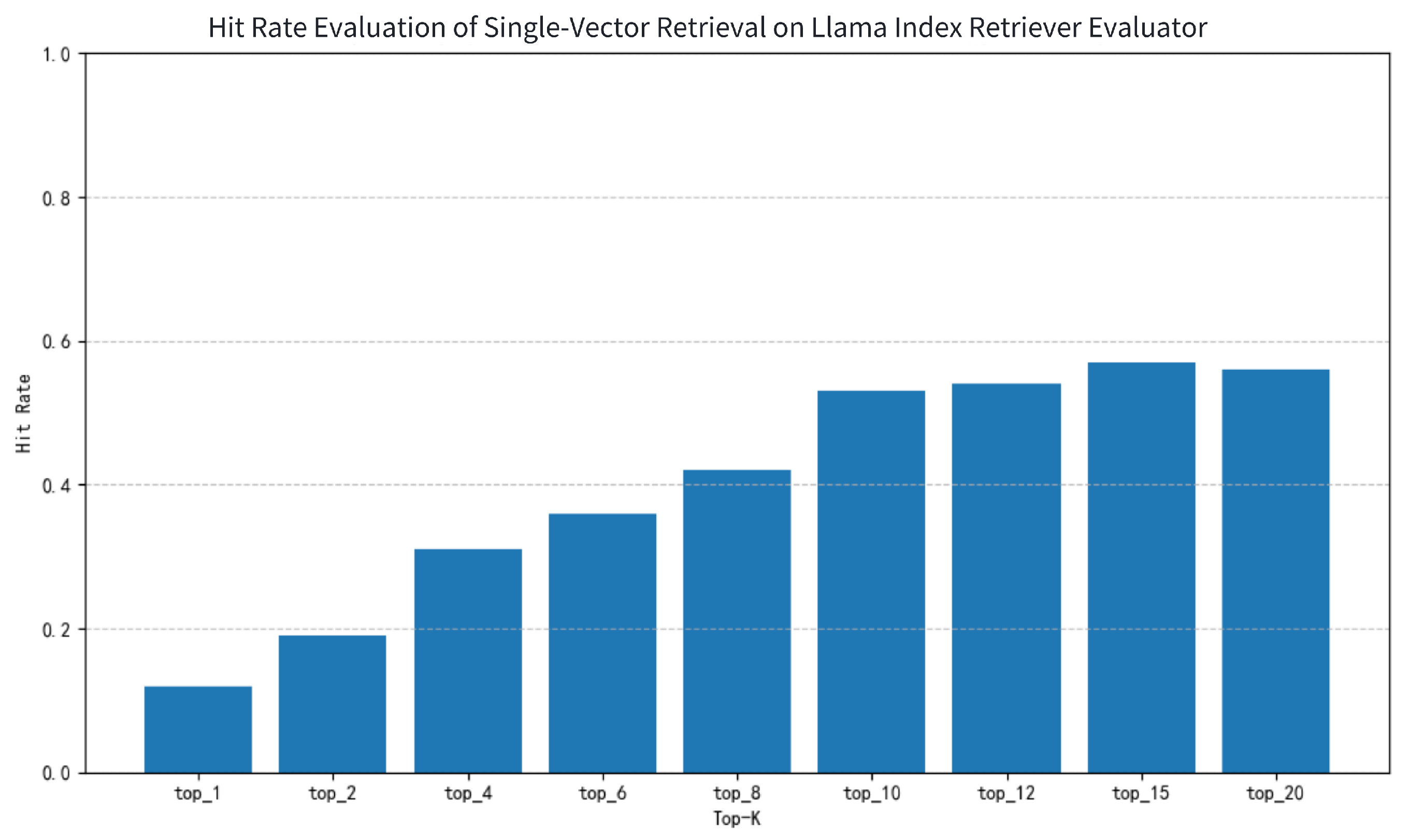
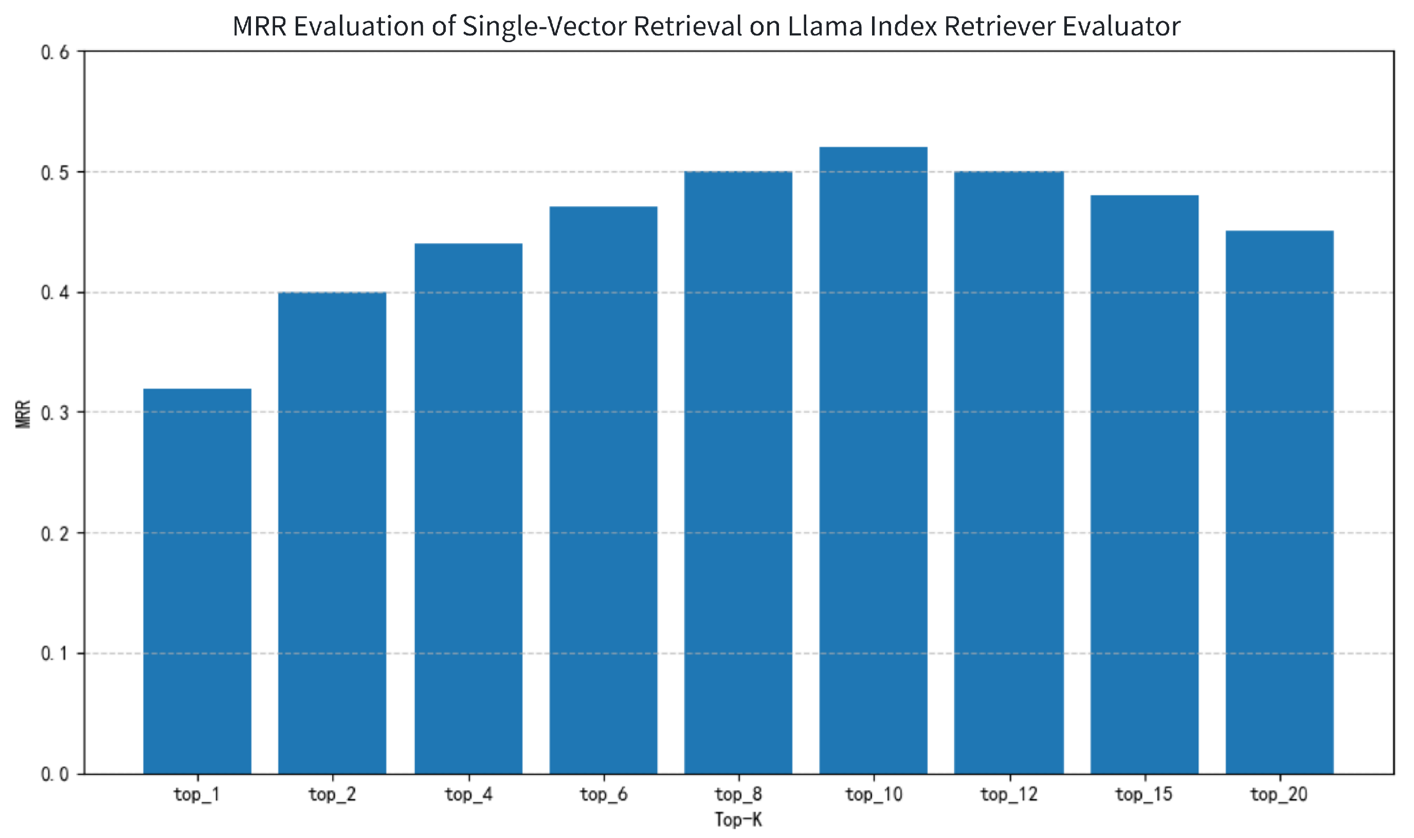
In the single-vector retrieval task, the retrieval model demonstrates a relatively stable Hit Rate under the Llama Index evaluation framework, as shown in Figure 11. The results indicate that as Top-K increases, the Hit Rate generally rises: it reaches 0.12 at Top-1, gradually increases to 0.57 at Top-15, and slightly decreases to 0.56 at Top-20, reflecting the positive impact of expanding the retrieval range. However, the improvement is not linear; the temporary drop at Top-12 suggests that the model may introduce ranking interference or redundant results in some samples, limiting further Hit Rate improvement.

The MRR evaluation, illustrated in Figure 12, shows that the DPR model exhibits strong top-ranked retrieval capability, reaching 0.32 at Top-1 and peaking at 0.52 at Top-10. This indicates that the model can rank correct documents high for most queries. Although MRR slightly drops after Top-12, it remains above 0.45 overall, demonstrating stable ranking precision even as Top-K increases. This trend confirms the practical usability of the DPR model in semantically dense matching tasks, especially for downstream tasks with high ranking quality requirements.

(2)

Re-ranking Model

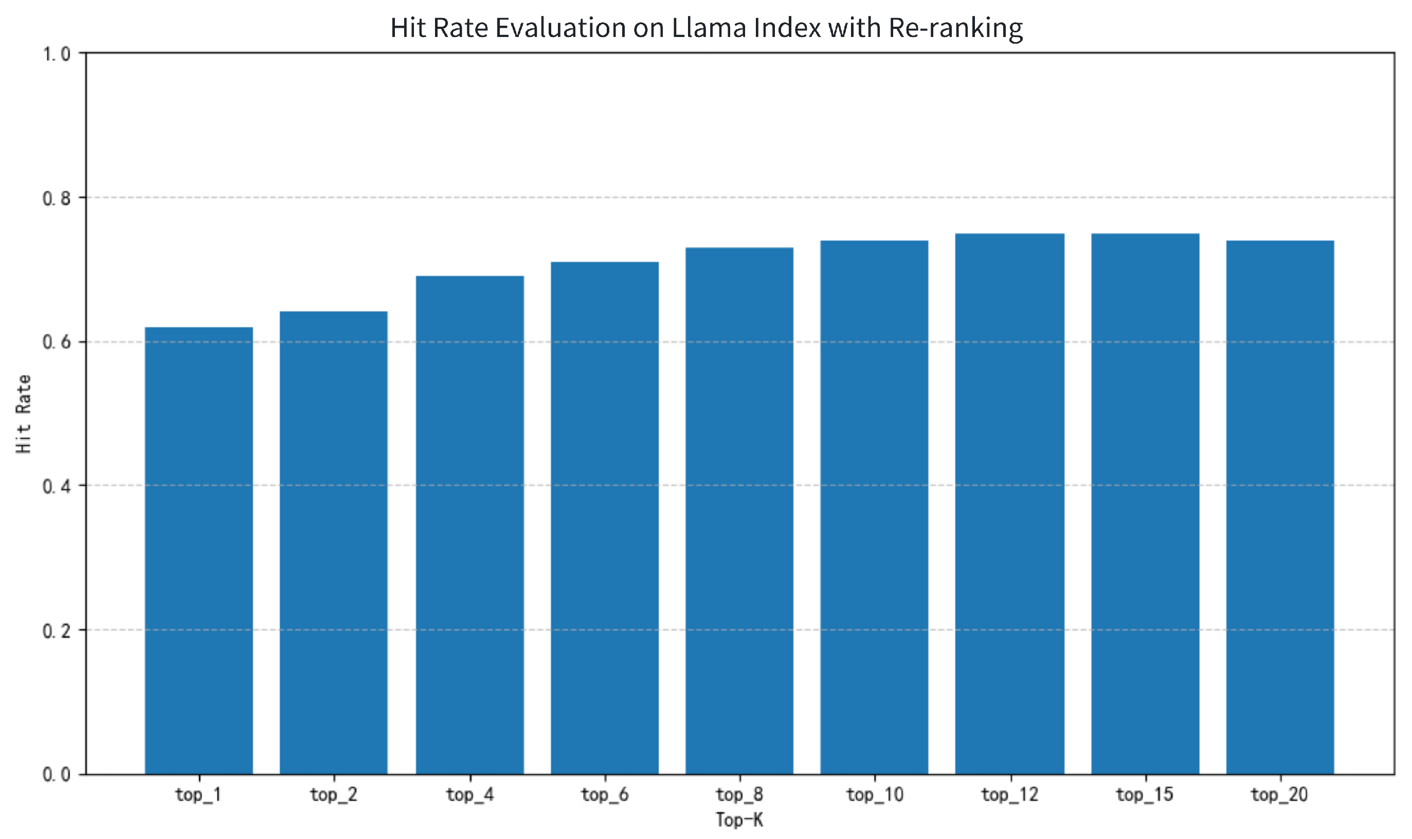
After initial single-vector retrieval, a re-ranking model is applied to refine the ranking of retrieved results. With the re-ranking module added, the Hit Rate under Llama Index is significantly enhanced, as shown in Figure 13. The overall curve becomes steeper and more stable compared with the baseline. Top-1 Hit Rate increases to 0.15, indicating improved first-position recall. As Top-K grows, the Hit Rate steadily rises, reaching 0.58 at Top-10 and peaking at 0.65 at Top-20, reflecting the Reranker’s effectiveness in reducing non-relevant documents and improving the discrimination of high-quality candidates. Overall, the two-stage retrieval strategy achieves a better balance between retrieval breadth and precision.

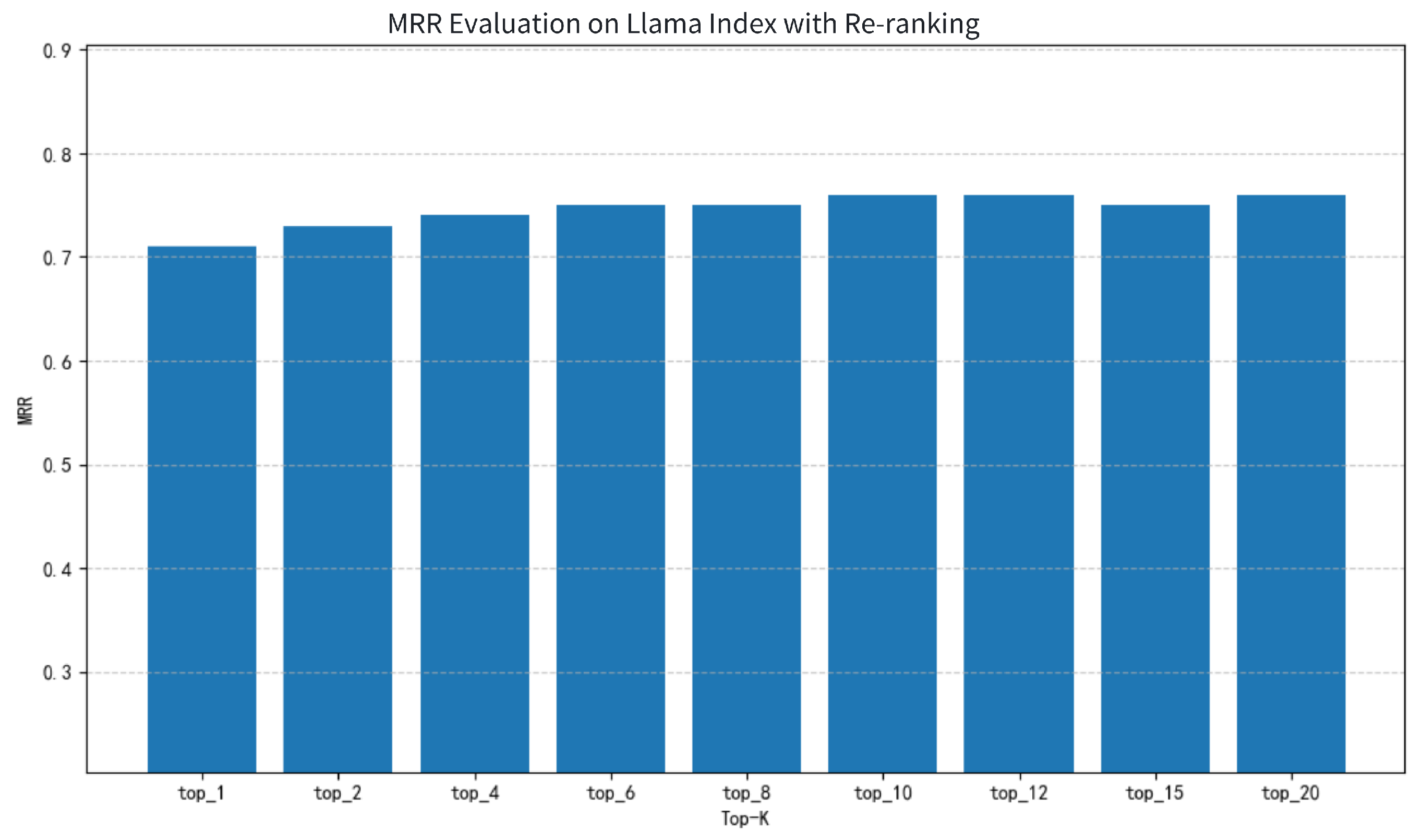
For MRR, the introduction of the re-ranking model significantly improves ranking quality, as shown in Figure 14. Top-1 MRR reaches 0.38, noticeably higher than the baseline without re-ranking, and peaks at 0.56 at Top-10. This demonstrates that the model effectively ranks correct results higher. These improvements highlight the Reranker’s advantage in fine-grained semantic understanding and its contribution to first-position recall in complex document retrieval tasks. Together with the Hit Rate enhancement, this shows that the Reranker substantially improves retrieval accuracy on top of DPR, making it a key component for high-performance retrieval systems.

(3)

Knowledge-Graph-Based Secondary Expansion

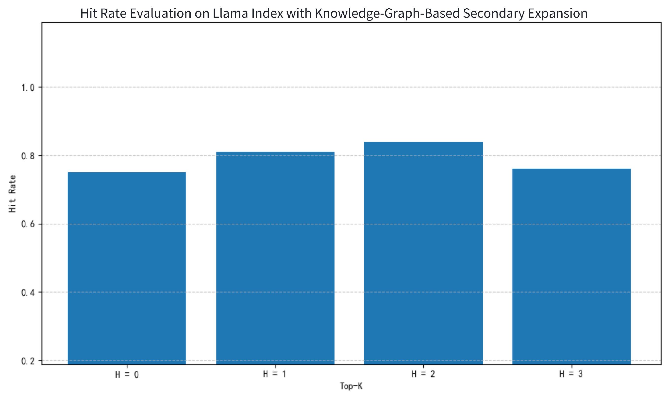
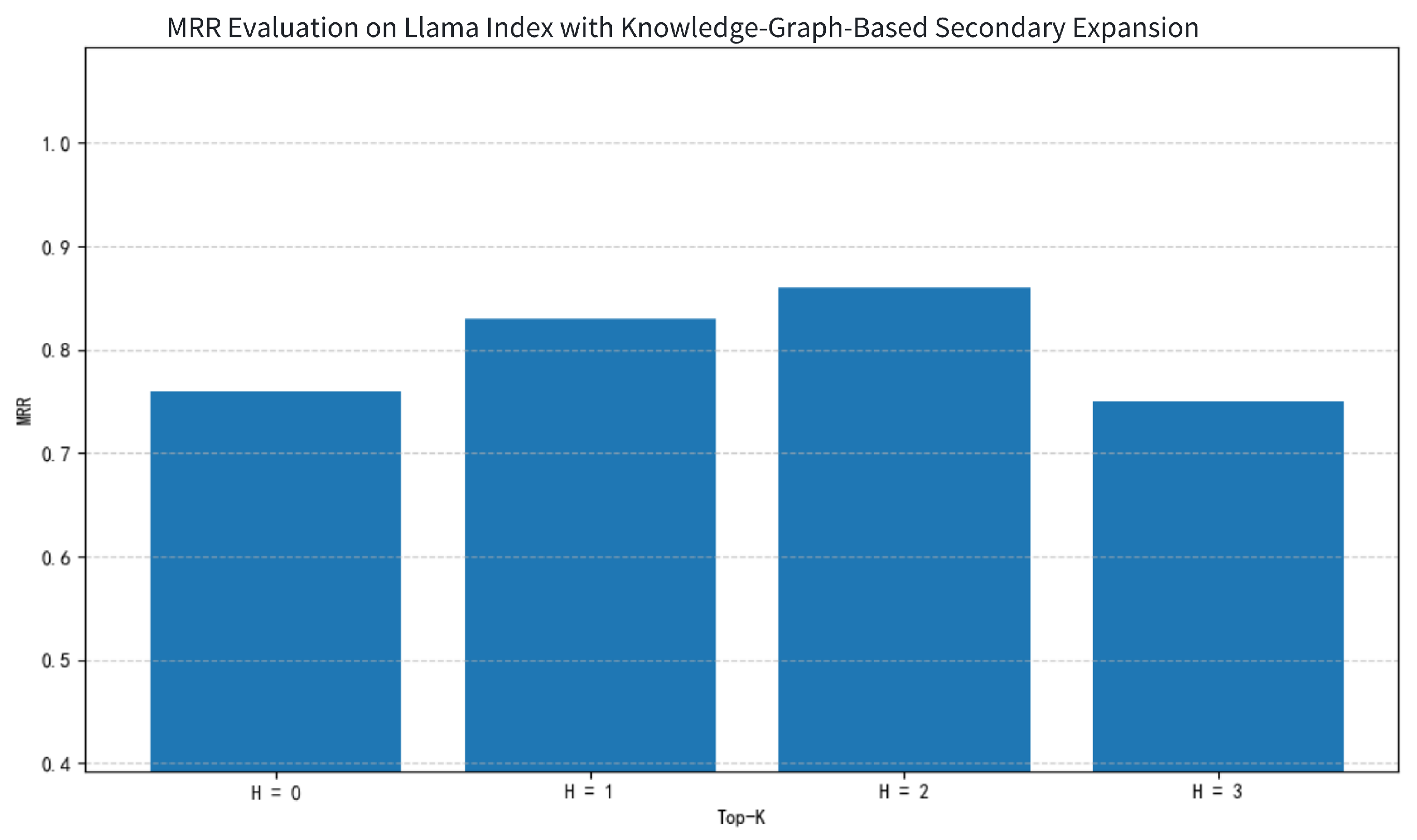
After introducing semantic expansion via a knowledge graph, the experimental results are shown in Figure 15 and Figure 16, indicating overall Hit Rate improvement, particularly in the one-hop and two-hop expansion stages. Compared with vector retrieval + re-ranking alone, adding one-hop knowledge-graph expansion allows the system to better associate semantically related concepts, with Hit Rate increasing from 0.75 to 0.81, and two-hop expansion further improving it to 0.84. This demonstrates that moderate semantic expansion helps capture deeper related information, enhancing the system’s understanding and recall of complex queries. At this stage, the knowledge graph effectively “extends semantic coverage,” which is particularly useful for retrieval tasks involving entity substitution, concept variation, or indirect reference. MRR trends similarly improve, especially in one-hop and two-hop expansions, indicating that knowledge-enhanced semantic representations not only improve recall but also significantly optimize ranking positions for relevant documents.

However, performance drops markedly after three-hop expansion, with Hit Rate returning close to the original vector retrieval + re-ranking level, and MRR also declining. This indicates that excessive expansion introduces semantic dilution and potential ranking interference. The degradation trend demonstrates that too many additional entities and noisy information can disrupt effective ranking and matching, diluting the semantic focus of the original query. Overall, the system exhibits a “rise-then-fall” trend with increasing expansion hops, suggesting that knowledge-graph expansion should be controlled within a reasonable range to maintain a balance between semantic relevance and information density, which is crucial for enhancing retrieval system performance.

5. Conclusions

In this paper, we proposed a lightweight vision–language model with dynamic feature down-sampling, specifically designed to address the computational challenges of high-resolution engineering imagery. Our model contributes an efficient dynamic compression mechanism that preserves fine-grained structural cues critical for engineering safety analysis, while significantly lowering computational overhead for practical deployment. Moreover, the integration of multi-scale feature modulation provides a more adaptive visual representation that benefits downstream structural assessment tasks. By adaptively compressing visual regions according to their information density, the model effectively preserves critical structural details while reducing redundant computation. The integration of a Vision Transformer-based encoder with a compact language model, together with a similarity-driven multi-scale feature selection strategy, enables efficient multimodal representation learning under resource-constrained conditions. Extensive experiments on multiple vision–language benchmarks demonstrate that our approach achieves competitive performance compared with larger-scale models while offering superior efficiency. Furthermore, ablation studies confirm the individual contributions of dynamic down-sampling and multi-scale feature selection.

In addition, we introduced Domain-Specific Fine-Tuning and Knowledge Augmentation to further enhance the model’s performance for bridge health diagnosis. Domain-specific fine-tuning on the Bridge-SHM dataset enabled the model to capture specialized terminology, structural patterns, and defect characteristics, significantly improving accuracy in bridge-specific visual question-answering tasks. Knowledge augmentation, through retrieval from external knowledge sources and semantic expansion via knowledge graphs, further enhanced the model’s reasoning and context-awareness, allowing it to provide more informed and precise diagnostic outputs. Collectively, these components ensure that the proposed framework is not only efficient but also highly adaptable and knowledge-enhanced, suitable for real-world structural health monitoring applications.

Despite these advantages, our current model still exhibits several limitations. First, the dynamic down-sampling strategy relies on handcrafted similarity metrics, which may not fully capture complex structural patterns in highly heterogeneous engineering imagery. In addition, cross-domain generalization remains a challenge, especially when transferring from standard benchmarks to diverse real-world engineering environments. Moreover, considering the safety-critical nature of bridge inspection, the automated damage detection process still carries inherent risks. The model may fail to recognize defects that do not produce clear visual deformation, leading to potentially unsafe false negatives. Furthermore, the current framework does not explicitly quantify prediction uncertainty, which limits its reliability in scenarios where ambiguous or subtle structural cues may mislead the diagnostic results. These issues highlight the need for uncertainty-aware mechanisms and enhanced safety guarantees before real-world deployment.

Looking forward, several research directions are worth exploring. One promising direction is the development of fully learnable or reinforcement-learning-based down-sampling policies that can adaptively determine the optimal compression strategy for different scenes. Another direction involves integrating stronger multimodal pre-training objectives or leveraging large-scale engineering-specific datasets to enhance domain adaptability. Moreover, future models could incorporate 3D geometric priors or physical constraints to better reason about structural components in engineering contexts. Finally, combining efficient vision–language models with edge computing or on-device deployment techniques may enable real-time analysis in practical industrial and engineering applications.

References

1. Sun, H.; Song, L.; Yu, Z. Bridge damage localization and quantification using deep learning and FEM static simulation. Mech. Syst. Signal Process. 2024, 211, 111177. [Google Scholar] [CrossRef]
2. Ngeljaratan, L.; Moustafa, M.A.; Sumarno, A.; Prasetyo, A.M.; Sari, D.P.; Maidina, M. Improved blob-based feature detection and refined matching algorithms for seismic structural health monitoring of bridges using a vision-based sensor system. Infrastructures 2024, 9, 97. [Google Scholar] [CrossRef]
3. D’Angelo, M.; Civera, M.; Giordano, P.F.; Borlenghi, P.; Ballio, F.; Limongelli, M.P.; Chiaia, B. Bridge collapses in Italy across the 21st century: Survey and statistical analysis. Struct. Infrastruct. Eng. 2025, 1–23. [Google Scholar] [CrossRef]
4. Bazrafshan, P.; Melag, K.; Ebrahimkhanlou, A. Semantic and lexical analysis of pre-trained vision language artificial intelligence models for automated image descriptions in civil engineering. AI Civ. Eng. 2025, 4, 17. [Google Scholar] [CrossRef]
5. Micozzi, F.; Morici, M.; Zona, A.; Dall’Asta, A. Vision-based structural monitoring: Application to a medium-span post-tensioned concrete bridge under vehicular traffic. Infrastructures 2023, 8, 152. [Google Scholar] [CrossRef]
6. Tang, S.; Chen, Z. Scale–space data augmentation for deep transfer learning of crack damage from small sized datasets. J. Nondestruct. Eval. 2020, 39, 70. [Google Scholar] [CrossRef]
7. Guo, L.; Li, R.; Jiang, B.; Shen, X. Automatic crack distress classification from concrete surface images using a novel deep-width network architecture. Neurocomputing 2020, 397, 383–392. [Google Scholar] [CrossRef]
8. Zhu, D.; Chen, J.; Shen, X.; Li, X.; Elhoseiny, M. Minigpt-4: Enhancing vision-language understanding with advanced large language models. arXiv 2023, arXiv:2304.10592. [Google Scholar]
9. Li, J.; Li, D.; Savarese, S.; Hoi, S. Blip-2: Bootstrapping language-image pre-training with frozen image encoders and large language models. In Proceedings of the International Conference on Machine Learning, Honolulu, HI, USA, 23–29 July 2023; pp. 19730–19742. [Google Scholar]
10. Yang, X. Bridge health monitoring and evaluation system. In Proceedings of the IOP Conference Series: Earth and Environmental Science; IOP Publishing: Bristol, UK, 2021; Volume 768, p. 012103. [Google Scholar]
11. Fu, Y.; Zhu, Y.; Hoang, T.; Mechitov, K.; Spencer, B.F., Jr. xImpact: Intelligent Wireless System for Cost-Effective Rapid Condition Assessment of Bridges Under Impacts. Sensors 2022, 22, 5701. [Google Scholar] [CrossRef]
12. Preethichandra, D.; Suntharavadivel, T.; Kalutara, P.; Piyathilaka, L.; Izhar, U. Influence of smart sensors on structural health monitoring systems and future asset management practices. Sensors 2023, 23, 8279. [Google Scholar] [CrossRef]
13. Flah, M.; Nunez, I.; Ben Chaabene, W.; Nehdi, M.L. Machine Learning Algorithms in Civil Structural Health Monitoring: A Systematic Review. Arch. Comput. Methods Eng. 2021, 28, 2621–2643. [Google Scholar] [CrossRef]
14. Okazaki, Y.; Okazaki, S.; Asamoto, S.; Chun, P.j. Applicability of machine learning to a crack model in concrete bridges. Comput.-Aided Civ. Infrastruct. Eng. 2020, 35, 775–792. [Google Scholar] [CrossRef]
15. Roy, S.; Yogi, B.; Majumdar, R.; Ghosh, P.; Das, S.K. Deep learning-based crack detection and prediction for structural health monitoring. Discov. Appl. Sci. 2025, 7, 674. [Google Scholar] [CrossRef]
16. Di Mucci, V.M.; Cardellicchio, A.; Ruggieri, S.; Nettis, A.; Renò, V.; Uva, G. Artificial intelligence in structural health management of existing bridges. Autom. Constr. 2024, 167, 105719. [Google Scholar] [CrossRef]
17. Jiménez Rios, A.; Plevris, V.; Nogal, M. Bridge management through digital twin-based anomaly detection systems: A systematic review. Front. Built Environ. 2023, 9, 1176621. [Google Scholar] [CrossRef]
18. Spencer, B.F., Jr.; Sim, S.H.; Kim, R.E.; Yoon, H. Advances in artificial intelligence for structural health monitoring: A comprehensive review. KSCE J. Civ. Eng. 2025, 29, 100203. [Google Scholar] [CrossRef]
19. Sharir, G.; Noy, A.; Zelnik-Manor, L. An image is worth 16x16 words, what is a video worth? arXiv 2021, arXiv:2103.13915. [Google Scholar] [CrossRef]
20. Radford, A.; Kim, J.W.; Hallacy, C.; Ramesh, A.; Goh, G.; Agarwal, S.; Sastry, G.; Askell, A.; Mishkin, P.; Clark, J.; et al. Learning transferable visual models from natural language supervision. In Proceedings of the International Conference on Machine Learning, Virtual, 18–24 July 2021; pp. 8748–8763. [Google Scholar]
21. Liu, H.; Li, C.; Wu, Q.; Lee, Y.J. Visual instruction tuning. Adv. Neural Inf. Process. Syst. 2023, 36, 34892–34916. [Google Scholar]
22. Liu, H.; Li, C.; Li, Y.; Lee, Y.J. Improved baselines with visual instruction tuning. In Proceedings of the the IEEE/CVF Conference on Computer Vision and Pattern Recognition, Seattle, WA, USA, 16–22 June 2024; pp. 26296–26306. [Google Scholar]
23. Li, Y. MOR-VIT: Efficient Vision Transformer with Mixture-of-Recursions. arXiv 2025, arXiv:2507.21761. [Google Scholar] [CrossRef]
24. Wu, Q.; Xu, W.; Liu, W.; Tan, T.; Liujianfeng, L.; Li, A.; Luan, J.; Wang, B.; Shang, S. Mobilevlm: A vision-language model for better intra-and inter-ui understanding. In Proceedings of the Findings of the Association for Computational Linguistics: EMNLP 2024, Miami, FL, USA, 12–16 November 2024; pp. 10231–10251. [Google Scholar]
25. Fan, H.; Xiong, B.; Mangalam, K.; Li, Y.; Yan, Z.; Malik, J.; Feichtenhofer, C. Multiscale vision transformers. In Proceedings of the IEEE/CVF International Conference on Computer Vision, Virtual, 11–17 October 2021; pp. 6824–6835. [Google Scholar]
26. Zhang, Y.; Fan, C.K.; Ma, J.; Zheng, W.; Huang, T.; Cheng, K.; Gudovskiy, D.; Okuno, T.; Nakata, Y.; Keutzer, K.; et al. Sparsevlm: Visual token sparsification for efficient vision-language model inference. arXiv 2024, arXiv:2410.04417. [Google Scholar]
27. Hu, E.J.; Shen, Y.; Wallis, P.; Allen-Zhu, Z.; Li, Y.; Wang, S.; Wang, L.; Chen, W. Lora: Low-rank adaptation of large language models. ICLR 2022, 1, 3. [Google Scholar]
28. Dettmers, T.; Pagnoni, A.; Holtzman, A.; Zettlemoyer, L. Qlora: Efficient finetuning of quantized llms. Adv. Neural Inf. Process. Syst. 2023, 36, 10088–10115. [Google Scholar]
29. Zhang, Q.; Chen, M.; Bukharin, A.; Karampatziakis, N.; He, P.; Cheng, Y.; Chen, W.; Zhao, T. Adalora: Adaptive budget allocation for parameter-efficient fine-tuning. arXiv 2023, arXiv:2303.10512. [Google Scholar]
30. Karpukhin, V.; Oguz, B.; Min, S.; Lewis, P.S.; Wu, L.; Edunov, S.; Chen, D.; Yih, W.t. Dense Passage Retrieval for Open-Domain Question Answering. In Proceedings of the Conference on Empirical Methods in Natural Language Processing, Online, 16–20 November 2020; pp. 6769–6781. [Google Scholar]
31. Reimers, N.; Gurevych, I. Sentence-bert: Sentence embeddings using siamese bert-networks. arXiv 2019, arXiv:1908.10084. [Google Scholar] [CrossRef]
32. Zhu, Y.; Xie, C.; Liang, S.; Zheng, B.; Guo, S. Focusllava: A coarse-to-fine approach for efficient and effective visual token compression. arXiv 2024, arXiv:2411.14228. [Google Scholar]
33. Rumelhart, D.E.; Hinton, G.E.; Williams, R.J. Learning Internal Representations by Error Propagation; Technical Report ICS-8506; Institute for Cognitive Science, University of California: San Diego, CA, USA, 1985. [Google Scholar]
34. Misra, D. Mish: A self regularized non-monotonic activation function. arXiv 2019, arXiv:1908.08681. [Google Scholar]
35. Xu, B.; Wang, N.; Chen, T.; Li, M. Empirical evaluation of rectified activations in convolutional network. arXiv 2015, arXiv:1505.00853. [Google Scholar] [CrossRef]
36. Hendrycks, D. Gaussian Error Linear Units (Gelus). arXiv 2016, arXiv:1606.08415. [Google Scholar]
37. Hudson, D.A.; Manning, C.D. Gqa: A new dataset for real-world visual reasoning and compositional question answering. In Proceedings of the IEEE/CVF Conference on Computer Vision and Pattern Recognition, Long Beach, CA, USA, 16–20 June 2019; pp. 6700–6709. [Google Scholar]
38. Lu, P.; Mishra, S.; Xia, T.; Qiu, L.; Chang, K.W.; Zhu, S.C.; Tafjord, O.; Clark, P.; Kalyan, A. Learn to explain: Multimodal reasoning via thought chains for science question answering. Adv. Neural Inf. Process. Syst. 2022, 35, 2507–2521. [Google Scholar]
39. Singh, A.; Natarajan, V.; Shah, M.; Jiang, Y.; Chen, X.; Batra, D.; Parikh, D.; Rohrbach, M. Towards vqa models that can read. In Proceedings of the the IEEE/CVF Conference on Computer Vision and Pattern Recognition, Long Beach, CA, USA, 16–20 June 2019; pp. 8317–8326. [Google Scholar]
40. Li, Y.; Du, Y.; Zhou, K.; Wang, J.; Zhao, W.X.; Wen, J.R. Evaluating object hallucination in large vision-language models. arXiv 2023, arXiv:2305.10355. [Google Scholar] [CrossRef]
41. Liu, Y.; Duan, H.; Zhang, Y.; Li, B.; Zhang, S.; Zhao, W.; Yuan, Y.; Wang, J.; He, C.; Liu, Z.; et al. Mmbench: Is your multi-modal model an all-around player? In Proceedings of the European Conference on Computer Vision, Milan, Italy, 29 September–4 October 2024; Springer: Berlin/Heidelberg, Germany, 2024; pp. 216–233. [Google Scholar]
42. Guia, J.; Soares, V.G.; Bernardino, J. Graph databases: Neo4j analysis. In Proceedings of the International Conference on Enterprise Information Systems, Porto, Portugal, 26–29 April 2017; pp. 351–356. [Google Scholar]
43. Javaheripi, M.; Bubeck, S.; Abdin, M.; Aneja, J.; Bubeck, S.; Mendes, C.C.T.; Chen, W.; Del Giorno, A.; Eldan, R.; Gopi, S.; et al. Phi-2: The surprising power of small language models. Microsoft Res. Blog 2023, 1, 3. [Google Scholar]
44. Bai, J.; Bai, S.; Chu, Y.; Cui, Z.; Dang, K.; Deng, X.; Fan, Y.; Ge, W.; Han, Y.; Huang, F.; et al. Qwen technical report. arXiv 2023, arXiv:2309.16609. [Google Scholar] [CrossRef]
Figure 1. Overall framework of our method. In Phase I, the workflow of our DL-VLM is presented. The DL-VLM integrates both visual and textual inputs. Image inputs are processed through region segmentation, visual encoding, feature mapping, and multi-scale downsampling and dynamic scale selection modules. Textual queries are encoded via a text encoder. The processed features are then aligned across modalities and fed into a LLM to generate the final natural language detection results along with corresponding coordinates. Phase II introduces domain-specific fine-tuning, in which the visual encoder is frozen while the visual projector is updated, and the LLM is adapted using LoRA-based low-rank optimization. This process enhances the model’s ability to recognize bridge-specific defects and engineering terminology while mitigating overfitting and reducing training cost. Phase III incorporates knowledge augmentation through dense retrieval and semantic reranking. Retrieved domain knowledge—encoded in structured triples and natural-language descriptions—is fused with multimodal features before entering the LLM, enabling more accurate reasoning and context-aware defect interpretation.
Bdcc 10 00003 g001
Figure 2. Feature Mapping and Alignment Module with Mish Activation.The module takes unaligned visual features ( 576 × 1024 ) from the visual encoder and applies a nonlinear transformation via an expansion layer ( 576 × 2048 ) and a compression layer ( 576 × 768 ), both using Mish activation. This projects visual features into a semantic space compatible with textual features, achieving cross-modal alignment and supporting subsequent multimodal fusion and reasoning.
Bdcc 10 00003 g002
Figure 3. Image Region Feature Differentiation. Regions in dashed boxes indicate low-information-density areas, mainly repetitive or uniform background, while unboxed regions represent high-information-density areas containing task-relevant details (e.g., bridge structures, piers).
Bdcc 10 00003 g003
Figure 4. Multiscale down-sampling. This module takes n raw image patch feature vectors X i = ( x 1 , x 2 , , x n ) as input and compute all the top K s informative subset D S ( i ) [ s ] for dynamic scale selection, where s = { 0 , 1 , 2 } .
Bdcc 10 00003 g004
Figure 5. Dynamic scale selection. This module adaptively determines the most informative feature resolution for each image region based on its semantic complexity. Instead of using a fixed downsampling ratio for all regions, this module dynamically selects the appropriate scale K s according to the distribution of token differentiation scores.
Bdcc 10 00003 g005
Figure 6. Two-Stage Training Pipeline.
Bdcc 10 00003 g006
Figure 7. Representative scenes from the Bridge-SHM dataset.
Bdcc 10 00003 g007
Figure 8. Example of the multi-turn vision–language data format.
Bdcc 10 00003 g008
Figure 9. Example of mild brightness-based data augmentation.
Bdcc 10 00003 g009
Figure 10. Examples of the QA Task.
Bdcc 10 00003 g010
Figure 11. Hit Rate Evaluation of Single-Vector Retrieval on Llama Index Retriever Evaluator.
Bdcc 10 00003 g011
Figure 12. MRR Evaluation of Single-Vector Retrieval on Llama Index Retriever Evaluator.
Bdcc 10 00003 g012
Figure 13. Hit Rate Evaluation on Llama Index with Re-ranking.
Bdcc 10 00003 g013
Figure 14. MRR Evaluation on Llama Index with Re-ranking.
Bdcc 10 00003 g014
Figure 15. Hit Rate Evaluation on Llama Index with Knowledge-Graph-Based Secondary Expansion.
Bdcc 10 00003 g015
Figure 16. MRR Evaluation on Llama Index with Knowledge-Graph-Based Secondary Expansion.
Bdcc 10 00003 g016