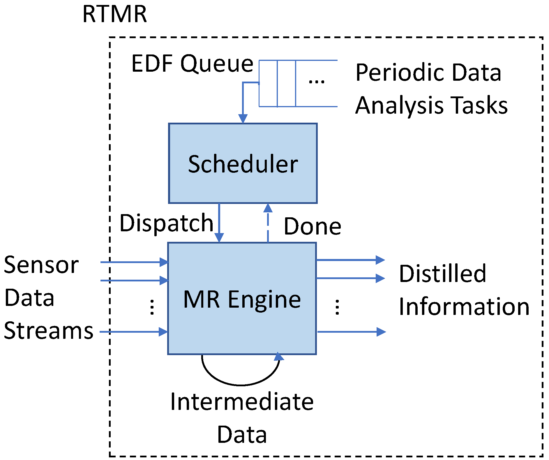
In this section, we implement a prototype RTMR system and evaluate the performance in a stepwise manner. We evaluate the performance of (1) the dynamic transfer rate allocation algorithm based on sensor data importance and (2) the timeliness of real-time data analytics tasks.
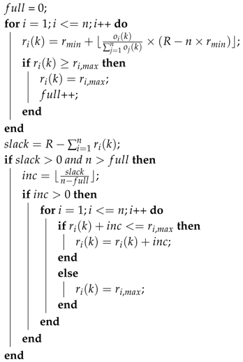
5.1. Cost-Effective Rate Allocation to IoT Devices
In this subsection, we implement and evaluate our dynamic service rate allocation algorithm (Algorithm 1) using several smartphones and a desktop PC equipped with a quad core Intel processor i7-4790 (3.6 GHz) and 16 GB main memory to emulate a low-end edge server specialized for image processing [
36] to demonstrate the real-world applicability of our system. To evaluate the E2E timeliness on different devices, we use 5 different smartphones: Huawei Honor 6, Galaxy S6, LG G3, Google Nexus 6, and Google Nexus 3 that transfer images to the edge server across busecure [
37], which is the public WiFi network on our campus with the nominal bandwidth of 144 Mbps. We have no privilege to reserve any channel or bandwidth, since busecure is the public WiFi network on our campus. Thus, providing any hard or soft real-time guarantee is impossible. Instead, we focus on optimizing the utility for sensor data transfer and analytics.
In this experiment, we set
fps (frames per second),
fps, and
fps. None of the smartphone we used can support more than 5 fps to take pictures and compress and transmit them. The control period for transfer rate adaptation is set to 10 s. All the smartphones transfer images to the edge server for 2 min. The image resolution is 720 × 486. (The image resolution instead of the transfer rate could be adjusted to enhance the total utility subject to our constraints specified in (
3)–(
5). This is reserved for future work.) The size of each image ranges between 4.9−10.2 KB after JPEG compression. The average face detection accuracy is 97.3%. Although our approach is not limited to a specific sensing and analytics application, we consider face detection as a case study. In that context,
is defined to be the number of human faces detected in the sensor data stream provided by embedded IoT device
. In this subsection, the E2E deadline for sensor data (i.e., image) transfer and analytics (i.e., face detection in this case study) is set to 100 ms.
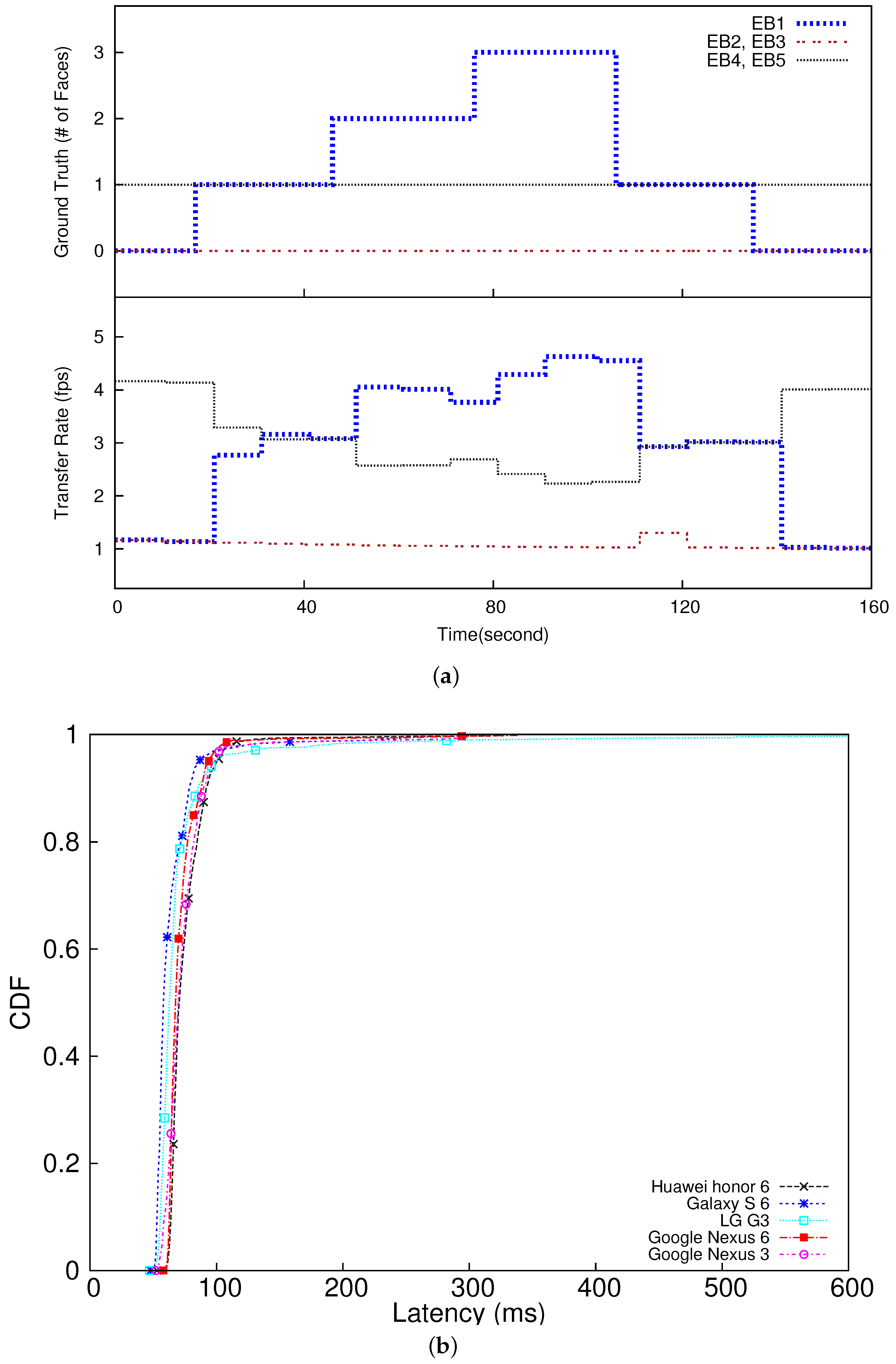
To verify the feasibility of dynamic rate adaptation based on data importance, we have created an experimental scenario such that each camera captures a certain number of faces in certain time intervals as depicted in the upper half of
Figure 7a. As shown in the lower half of
Figure 7a, the transfer rates of the embedded devices (smartphones) are dynamically adapted in proportion to their data importance values (the numbers of detected faces) effectively tracking the changes in the ground truth. Initially, embedded devices 4 and 5 (EB4 and EB5 in the figure) are assigned the highest transfer rate, because each of them is configured to continuously take one face throughout the 2 min experiment. On the other hand, the other devices detect no face at the beginning. However, the rate of EB4 and EB5 is reduced as the edge server detects an increasing number of faces in the image stream provided by EB1, and accordingly increases EB1’s rate. The rate of EB4 and EB5 is increased again as EB1 detects fewer faces later in the experiment. Therefore, from
Figure 7, we observe that our rate allocation effectively reflects the data importance changes by dynamically adapting the transfer rates assigned to the embedded IoT devices in proportion to their relative data importance to optimize the utility. In this case study, our approach enhances the utility, i.e., the total number of faces delivered to the edge server, by 38% compared to the baseline approach unaware of data importance and assigns the same transfer rate to all the smartphones, which is the de facto standard in visual surveillance [
38,
39].
In this case study, the 95 percentile E2E latency of the slowest smartphone is 100 ms (equal to the E2E deadline) as plotted in
Figure 7 and summarized in
Table 1. The network latency ranges between 14 –36 ms. The rest of the latency is caused by real-time data analytics. Separate from the performance results in
Figure 7 and
Table 1, we have also executed the face detection task 100 times on the fastest smartphone that we have (Galaxy S6) without offloading the task to the edge server, in which we have found the 95 percentile latency is 309 ms. Based on this result and
Table 1, we observe that our approach leveraging the edge server decreases the 95 percentile E2E latency by 3.09x−3.59x compared to another baseline, in which each smartphone performs data analytics on its own with no offloading. In fact, a majority of IoT devices could be much less powerful than smartphones. Also, real-time data analytics may need to deal with bigger sensor data and more complex data analysis; therefore, embedded IoT devices may suffer from considerably longer latency, if compute-intensive tasks are executed on them. These observations further motivate real-time data analytics in the edge server.
5.2. Scheduling Real-Time Data Analysis Tasks
In this subsection, we assume that sensor data are efficiently delivered to RTMR at the network edge. (For example, our approach based on data importance can be integrated with the emerging 5 G or Gbps WiFi technology that significantly decreases the latency, enhancing the throughput.) In fact, it is possible to configure a real-time data analytics system such that a relatively low-end edge server handles specific tasks, e.g., face detection, within short deadlines, while a more powerful edge server performs more comprehensive, in-depth data analytics. (Efficient partitioning of real-time data analytics tasks among IoT devices and edge servers is beyond the scope of this paper. An in-depth research is reserved for future work.) Therefore, we evaluate the real-time performance of RTMR by running benchmarks associated with timing constraints for much bigger input sensor data than those used in
Section 5.1.
For performance evaluation, the following popular data analytics benchmarks [
20] are adapted to model periodic real-time data analysis tasks.
Histogram (HG): A histogram is a fundamental method for a graphical representation of any data distribution. In this paper, we consider image histograms that plot the number of pixels for each tonal value to support fundamental analysis in data-intensive real-time applications, e.g., cognitive assistance, traffic control, or visual surveillance. (HG is not limited to image data but generally applicable to the other types of data, e.g., sensor readings.) The input of this periodic task is a large image with pixels per task period. The input data size processed per period is approximately 1.4 GB.
Linear Regression (LR): Linear regression is useful for real-time data analytics. For example, it can be applied to predict sensor data values via time series analysis. In LR, points in two dimensional space, totaling 518 MB, are used as the input per task period to model the approximately linear relation between x and y via LR.
Matrix Multiplication (MM): MM is heavily used in various big data and IoT applications, such as cognitive assistance, autonomous driving, and scientific applications. In this paper, MM multiplies two matrices together per task period. Each input matrix is 16 MB. The output matrix is 16 MB too.
K-means clustering (KM): This is an important data mining algorithm for clustering. For example, it can be used to cluster mobile users based on their locations for real-time location-based services. It partitions ℓ observations into k clusters (usually ) such that each observation belongs to the cluster with the nearest mean. The input of the k-means task is points in two dimensional space, totaling 77 MB, per task period.
In this paper, we generate new data per period to maximize the workload to stress-test RTMR under a worst-case setting. In fact, some histograms and sub-matrices may not change between two consecutive periods when, for example, only part of images used for cognitive assistance or autonomous driving changes. Also, linear regression and k-means clustering can be performed incrementally between consecutive periods. We take this approach, since it is required to design a real-time scheduling framework considering a worst-case scenario to support the predictability [
24]. In the future, we could use, for example, average execution times for a probabilistic assurance of timeliness. However, this is a complex issue and beyond the scope of this paper. It is reserved as a future work.
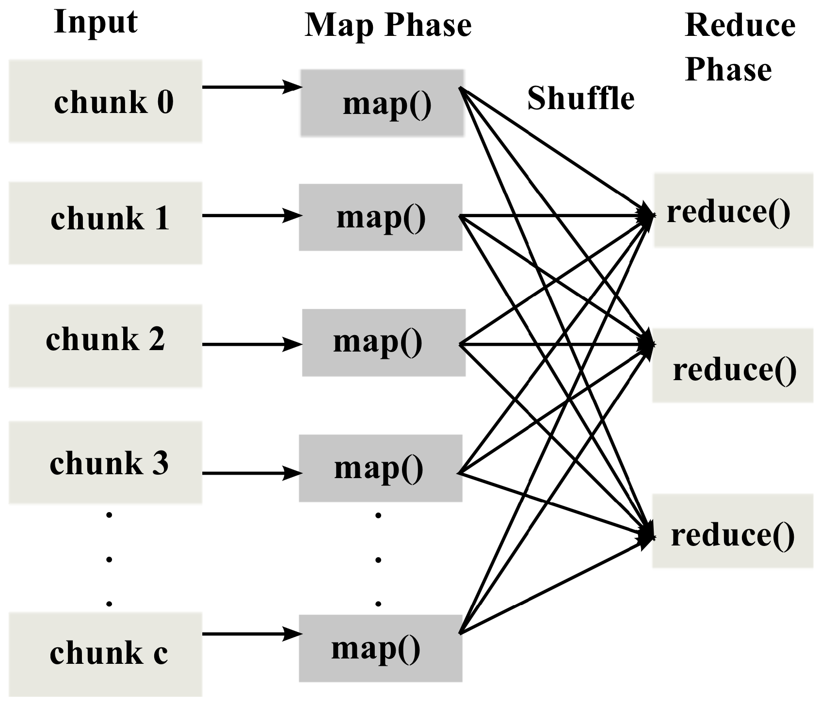
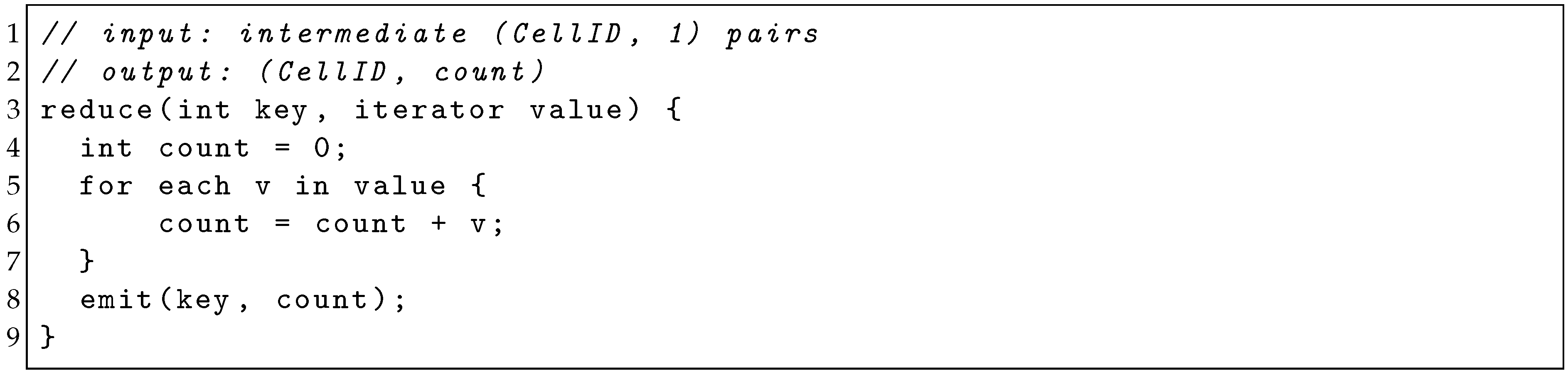
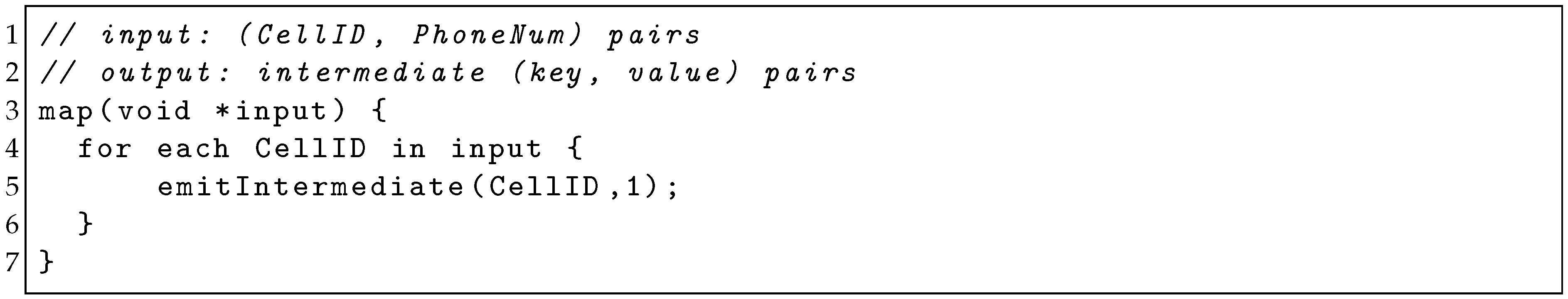
All the benchmarks are reductive; that is, the size of the intermediate/output data of all the benchmarks is not bigger than that of the input data. Among the tested benchmarks, only KM consists of more than one pair of map-reduce phases. Specifically, it is implemented as a series of seven pairs of iterative map and reduce phases. However, it generates no additional intermediate/output data; it only finds new
k means and updates the cluster membership of each point according to the new means in each pair of the map and reduce phases. For the tested benchmarks, enough memory is reserved as discussed in
Section 4.
Our system used for performance evaluation of RTMR is a Linux machine with two AMD Opteron 6272 processors, each of which has 16 cores running at 2.1 GHz. There is a 48 KB L1 cache and 1 MB L2 cache per core. In addition, there is a 16 MB L3 cache shared among the cores. Out of the 32 cores, one core is dedicated to the real-time scheduler and another core is exclusively used to generate periodic jobs of the real-time data analysis tasks. The remaining 30 cores are used to process the generated real-time data analysis jobs. The system has 32 GB memory.
Using the micro-benchmarks, we profile the maximum (observed) execution times of the tested benchmarks including the computation and data access latency, perform the schedulability analysis of real-time data management tasks offline based on the maximum execution times, and empirically verify whether the deadlines can be met for several sets of real-time data analysis tasks generated using the micro-benchmarks. Specifically, one benchmark is run 20 times offline using randomly generated data. The maximum latency among the 20 runs is used for the schedulability test.
Table 2 shows the maximum execution times of the benchmarks derived offline. As the number of cores to process real-time data analysis tasks,
m, is increased from 1 to 30, the maximum execution times of the HG, LR, MM, and KM are decreased by over 12, 4.1, 17.7, and 4.3 times, respectively. In HG and MM, load balancing among the cores is straightforward. As a result, the maximum execution time is decreased significantly for the increasing number of the cores used for real-time data analytics. Notably, LR’s maximum execution time in
Table 2 decreases substantially only after
. For
, the hardware parallelism provided by the employed CPU cores is not enough to considerably speed up LR. On the other hand, the decrease of KM’s maximum execution time in
Table 2 becomes marginal when
. In KM, individual points are often re-clustered and moved among different clusters until clustering is optimized in terms of the distance of each point to the closest mean. Thus, the cluster sizes may vary dynamically depending on the distribution of input points between the consecutive map/reduce phases. As a result, threads may suffer from load imbalance. Thus, using more cores does not necessarily decrease the maximum execution time of KM significantly.
For performance evaluation, we intend to design a task set with as short deadlines as possible. We have considered the six task sets in
Table 3 where the relative deadlines become shorter from
to
. We consider these task sets to analyze their schedulability for different numbers of cores subject to the two conditions specified in (
8) and (
9). In each task set, a longer deadline is assigned to a task with the larger maximum execution time. Also, in each task set, we have picked task periods (i.e., relative deadlines) such that the longest period in each task set is no more than twice longer than the shortest period in the task set to model real-time data analysis tasks that need to be executed relatively close to each other. In
, the tightest possible relative deadlines are picked subject to these constraints in addition to (
8) and (
9). The maximum execution times and relative deadlines of
for 30 cores are shown in the last column and row in
Table 2 and
Table 3, respectively. The maximum total utilization of
for 30 cores is set to 1 in (
8). Assigning shorter deadlines or bigger data to the tasks in
incurs deadline misses.
Table 4 shows the results of the schedulability tests for
–
). In
Table 4, ‘yes’ means a task set is schedulable (i.e., all deadlines will be met) for a specific number of cores used to run HG, LR, MM, and KM. We present the performance results for
that has the shortest deadlines and, therefore, it is only schedulable when
as shown in
Table 4. All four periodic benchmark tasks, i.e., HG, LR, KM, and MM tasks in
, simultaneously release their first jobs at time 0 and continue to generate jobs according to their periods specified in the last row of
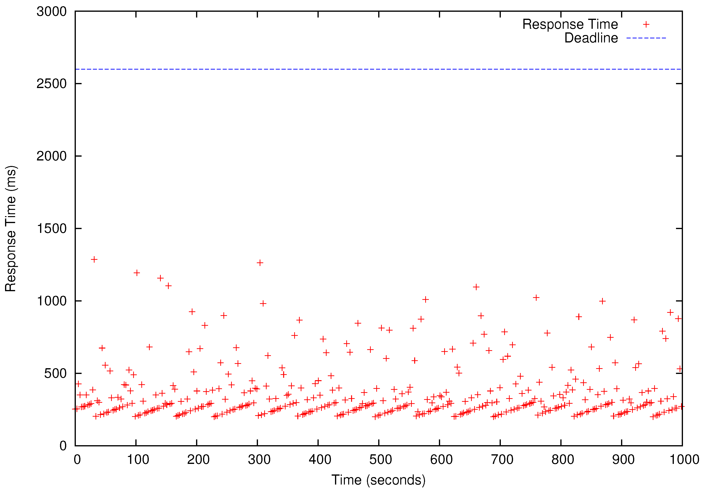
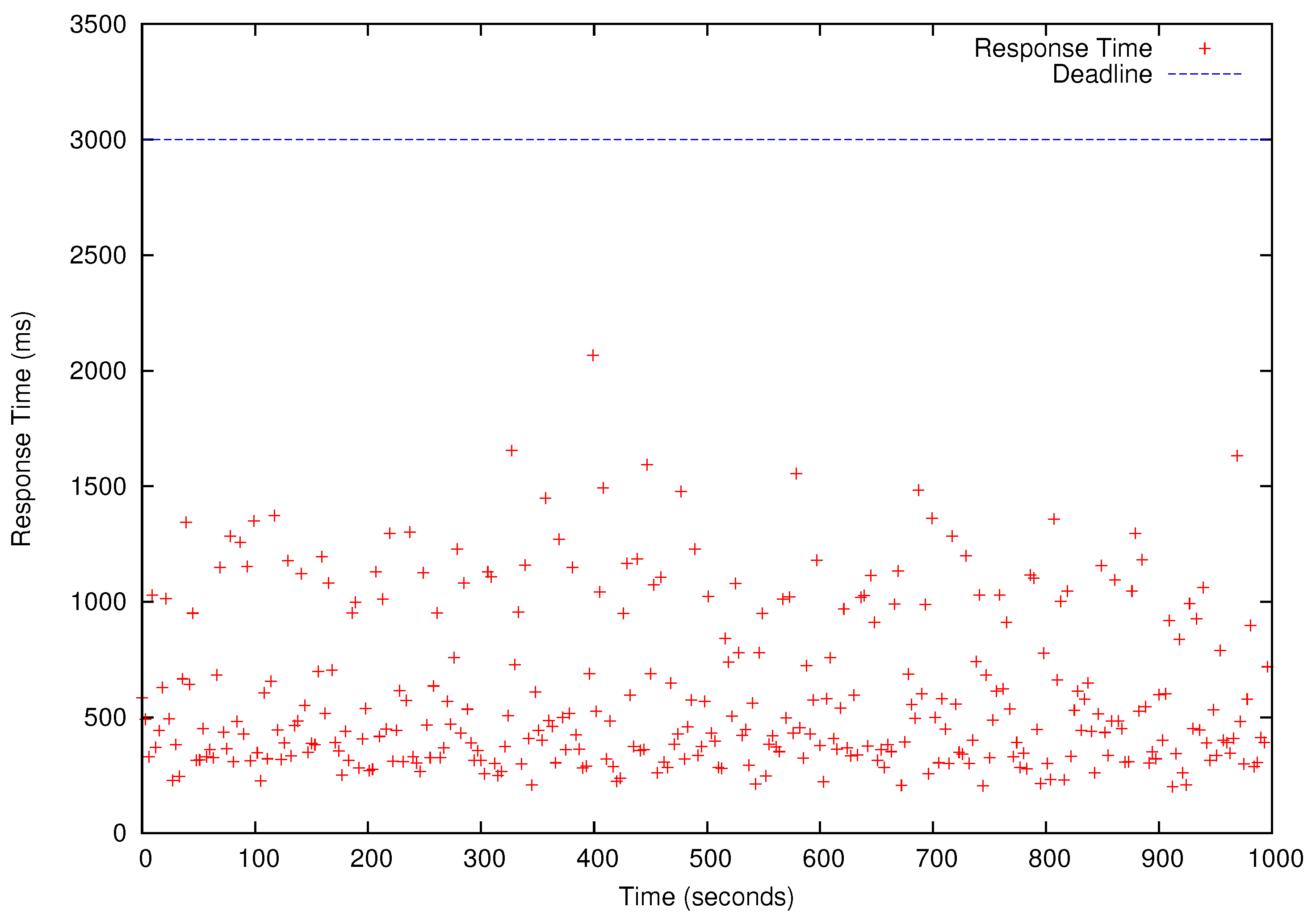
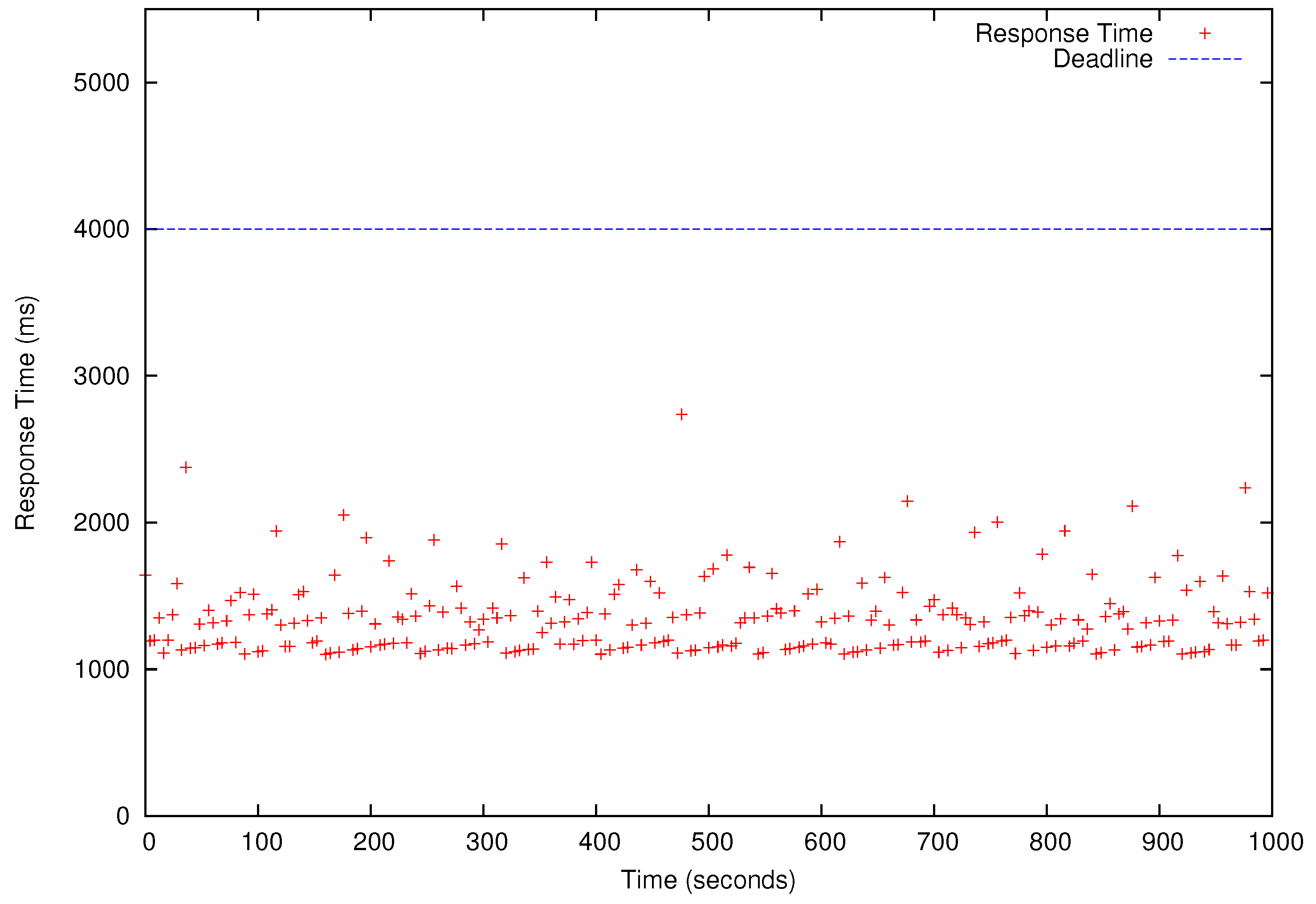
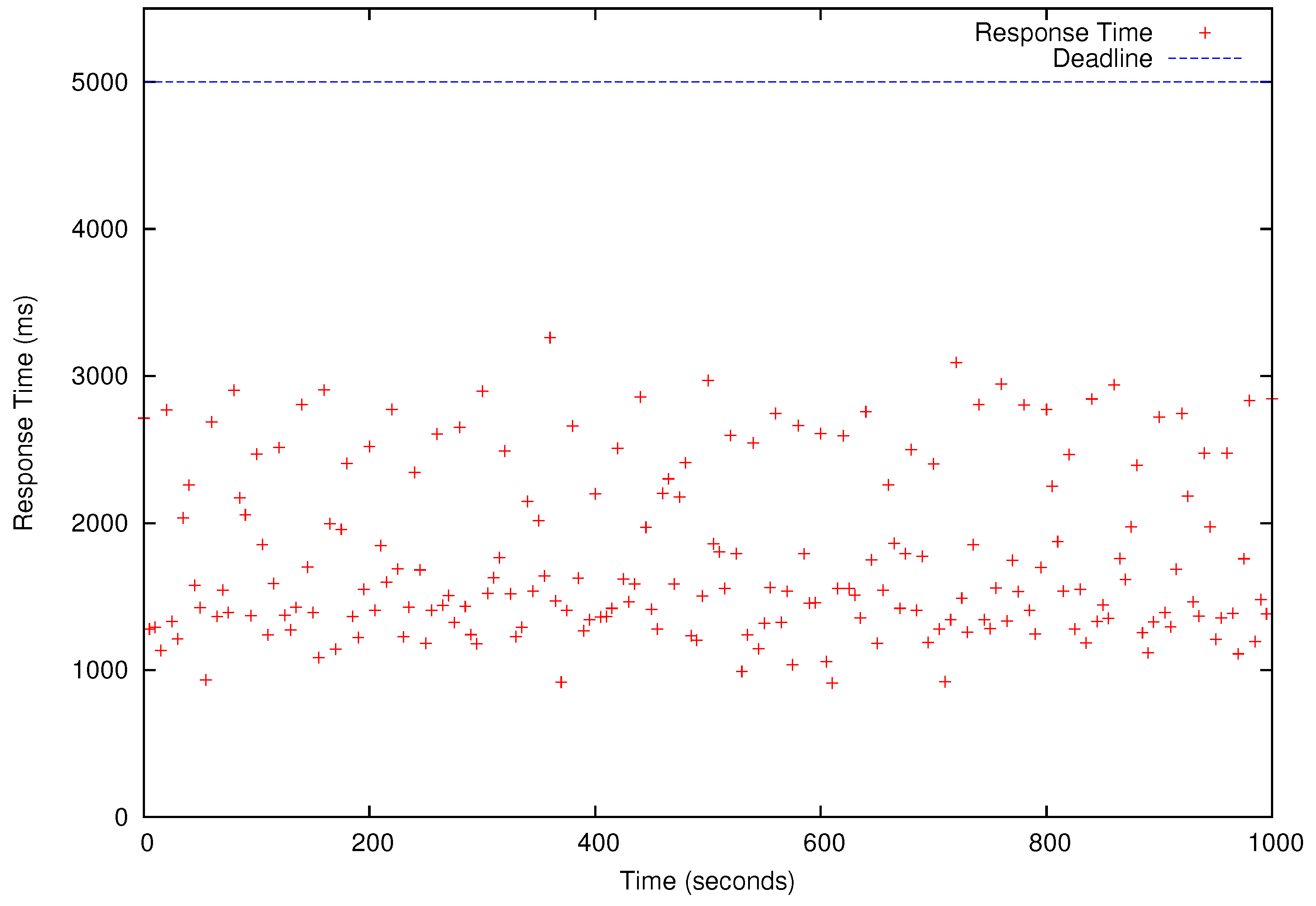
Table 3 for 1000 s. As shown in
Figure 8,
Figure 9,
Figure 10 and
Figure 11, all deadlines of the periodic real-time data analysis tasks in
are met. In total, more than 0.72 TB of data are processed in a 1000 s experimental run, which is projected to be over 62 TB/day.
In this paper, Phoenix [
20] is used as the baseline. It is closest to RTMR in that it is a state-of-the-art in-memory, multi-core map-reduce system unlike the other approaches mainly based on Hadoop (discussed in
Section 6). However, it has missed most deadlines of
for several reasons (although it meets the deadlines for light workloads, such as
using 30 cores). First, it is timing agnostic and only supports FIFO scheduling as discussed before. Further, it reads input data from and writes output to secondary storage without supporting input sensor data streaming into memory. Neither does it support in-memory pipelining of intermediate data for iterative tasks. As a result, a single operation to read input data from disk (write output to disk) takes 38 ms–1.35 s (71 ms–1.14 s) for the tested benchmarks.
In
Figure 8,
Figure 9,
Figure 10 and
Figure 11, we also observe that the periodic real-time data analysis jobs finish earlier than the deadlines due to the pessimistic real-time scheduling needed to meet the timing constraints. Notably, simply using advanced real-time scheduling techniques that support intra-task parallelism, e.g., [
34,
35], does not necessarily enhance the utilization. For example, the best known capacity augmentation bound of any global scheduler for tasks modeled as parallel directed acyclic graphs is 2.618 [
35]. Hence, the total utilization of the task set should be no more than
and the worst-case critical-path length of an arbitrary task
(i.e., the maximum execution time of
for an infinite number of cores) in the task set cannot exceed
of
to meet the deadlines.
Overall, our system design and experimental results serve as proof of concept for real-time big sensor data analytics. Our work presented in this paper opens up many research issues, e.g., more advanced scheduling, load balancing, execution time analysis, and real-time data analysis techniques, to efficiently extract value-added information from big sensor data in a timely manner.


