Numerical and Experimental Study of Flutter in a Realistic Labyrinth Seal ^†

Abstract

Labyrinth seals are commonly used in turbomachinery in order to control leakage flows. Flutter is one of the most dangerous potential issues for them, leading to High Cycle Fatigue (HCF) life considerations or even mechanical failure. This phenomenon depends on the interaction between aerodynamics and structural dynamics; mainly due to the very high uncertainties regarding the details of the fluid flow through the component, it is very hard to predict accurately. In 2014, as part of the E-Break research project funded by the European Union (EU), an experimental campaign regarding the flutter behaviour of labyrinth seals was conducted at “Centro de Tecnologias Aeronauticas” (CTA). During this campaign, three realistic seals were tested at different rotational speeds, and the pressure ratio where the flutter onset appeared was determined. The test was reproduced using a linearised uncoupled structural-fluid methodology of analysis based on Computational Fluid Dynamics (CFD) simulations, with results only in moderate agreement with experimental data. A procedure to adjust the CFD simulations to the steady flow measurements was developed. Once this method was applied, the matching between flutter predictions and the measured data improved, but some discrepancies could still be found. Finally, a set of simulations to retain the influence of the external cavities was run, which further improved the agreement with the testing data.

1. Introduction

Leakage flows in the radial gaps between static and rotating parts very significantly affect the performance of turbomachinery. Labyrinth seals are commonly used in order to reduce these flows. These seals are composed of a number of radial fins, which delimit small cavities between them. As a result, leakage flows undergo successive contractions and expansions as they pass through the fin tip or cavity region, leading to substantial losses of stagnation pressure and ultimately to a smaller mass flow than a simple slot. The performance of the component is noticeably difficult to predict accurately, in part due to the complexity of the flow (regions with very different Mach numbers, complex vortex structures and separated flow) and in part due to the very high sensitivity to manufacturing tolerances (typical gap values are in the 0.1–0.4 mm range).

One potentially severe issue that labyrinth seals may find is flutter, as documented decades ago by Lewis et al. [1]. Their research illustrates how vibration induced by aeroelastic instabilities may lead to the mechanical failure of the seal. The phenomenon has been studied by a number of authors, beginning with the works of Ehrich [2] and Alford [3], which provide a conceptual description of the problem and formulate simplified analytical models. Some years later, Abbot confirmed some of their main conclusions with experimental and numerical studies [4]. Thanks to the increase in computational power, the past decade saw the appearance of some analysis based on CFD simulations, often supported with additional experimental studies, such as those from di Mare et al. [5] and Miura et al. [6]. However, some authors such as Corral, Vega and Greco [7,8,9] continued with the analytical research of the phenomenon developing a new simplified model that describe the physics of the problem more accurately than its predecessors. The model was recently validated [10] against the experimental data described in [6].

Additionally, in recent years, there has been a growing interest in the industry about the topic, with different EU research projects focused on experimental campaigns in order to provide more insight into the phenomenon and produce good-quality data for numerical method validation. The work presented here takes the testing campaign performed by one of those projects (E-Break) as a reference for a set of CFD-based simulations, which successfully reproduce the measurements. One of the main achievements of the simulations is to account for the individual effect of external cavities over the seal structure, an effect that current simplified models ignore.

2. Experimental Set-Up and Procedure

E-Break (2010–2014) was a collaborative project co-funded by the EU with a work package focused on the study of flutter in labyrinth seals, relying on a comprehensive testing campaign. The main targets of the project were to gain a physical understanding of the phenomenon and to provide a set of good-quality experimental data, both of stable and unstable cases, to allow the validation of the tools and methodologies of analysis employed by the different partners. For that purpose, an unstable three-fins labyrinth seal was designed to act as the reference, and different techniques were employed to stabilise it, including changes in the operating point, geometry modifications and the addition of mechanical friction through dampers.

The aforementioned experimental campaign was conducted at Centro de Tecnologías Aeronáuticas (CTA) in Zamudio (Spain), a research institute with more than 20 years of experience in aerodynamic rigs for Low Pressure Turbines. They have also collaborated on other aeroelasticity projects such as FUTURE [11]. These cold flow facilities are designed for turbine rig testing, usually powered by the air flux provided by the compression system, making it difficult to adapt the facility interface to labyrinth seal testing. This restriction imposed the necessity to install a complete turbine rig to extract energy from the air flux and power the seal, eventually attached to the turbine disk.

The instrumentation of the rig allowed determining both the steady state and the flutter appearance. Regarding the steady field magnitudes, the seal mass flow, static pressure at both inter-fin cavities and external high-pressure side (HPS) and low-pressure side (LPS) cavities, static temperatures and the shaft speed were recorded to describe the seal operating point. With regard to the unsteady magnitudes, dynamic pressure sensors were located in the inter-fin cavities, and a number of dynamic strain gauges were installed in the seal specimen in order to monitor the vibration amplitudes and detect the flutter onset. A sketch of the rig and instrumentation positioning is shown in Figure 1. Note that the flow direction across the seal is from right (HPS) to left (LPS).

Two main parameters were controlled while testing, namely, the rotation speed of the disk and the feed pressure to the HPS chamber. The testing procedure, described in Figure 2, consisted in setting the rotation speed of the disk to a chosen value, which will be kept constant thereafter, imposing a zero-mass flow state (i.e., set the feeding pressure to ambient value), and then increasing the feeding pressure giving small steps. After each of these steps, the time to reach a stable regime was waited, and then, the different sensor’s measurements were recorded. The process was repeated until the strain gauges were able to detect vibration amplitudes above the established safety limits, the moment at which the test was concluded. For each of the instabilities observed, the operating conditions, vibration frequency, nodal diameter (ND) and travelling wave sense were determined, allowing an easy comparison with the numerical results.

Different seal geometries were tested, as depicted in Figure 3. The first specimen, which will be referred to as the baseline, is a three-fin geometry that corresponds to the aforementioned unstable seal selected for this project. The second geometry is the result of removing the left-most fin and cavity from the baseline configuration, yielding a two-fin seal. Additionally, a third seal not included in this work was tested in the E-Break campaign.

3. Methodology

The methodology employed in the flutter calculations presented here relies on a linearised uncoupled formulation of the unsteady vibration problem [12] (see Figure 4). This approach, widespread in the industry, simplifies the problem and significantly reduces the computational cost. Two main assumptions are behind this methodology. First, we consider that aeroelastic modes are essentially the same as the purely structural modes. Second, to linearise the unsteady problem equations, we assume that vibration amplitudes are small enough so that the fluid field can be decomposed in a base field plus a series of small perturbations. From the operational point of view, it involves performing a modal analysis of the structure to obtain the modal displacements and frequencies, a non-linear steady CFD simulation that will act as the base solution for the linearised problem, and finally an unsteady linearised CFD simulation where the previously calculated modal shapes and frequencies are imposed. As a result, an unsteady pressure field is obtained that, together with the modal displacements, eventually allows us to compute the work per cycle over the structural displacements imposed. The work per cycle can be converted to an aerodynamic critical damping ratio $\xi$ with the following expression:

$$\xi =\frac{W}{2\pi \omega M}$$

(1)

where W represents the work per cycle, $\omega$ is the modal angular frequency (rad/s), and M is the modal mass. The sign of the aerodynamic damping will determine the stability of the mode. According to our sign criteria, a negative value means that energy is being transferred from the flow to the structure, that is, the flutter.

The structural modes are obtained with a 3-dimensional pre-stressed modal analysis performed with our in-house solver Xipetotec [13]. To reduce the computational cost, the solid domain analysed consists of a sector of 18 degrees, small enough to study the nodal diameters of interest. The mesh has been generated as a 30-planes circumferential extrusion of a 2-dimensional grid to yield a mesh made of tetrahedrons with about 130,000 nodes (see Figure 5a). Regarding boundary conditions, depicted in Figure 5b, it should be mentioned that cyclic symmetry is employed (orange and fuchsia faces), shaft rotation imposed, aerodynamic loads considered over every wetted surface (transparent faces) and a series of displacement constraints imposed to model the seal attachment to the disk. Specifically, axial displacements have been restricted in all the face of contacts between the seal and disk (blue face), and a 3-degrees-of-freedom punctual constraint has been added to simulate the bolt.

The steady fluid problem is solved with ITP’s in-house CFD code Mu²s²t [14], a solver for the fully non-linear RANS equations which counts with a linearised version that allows us to solve the unsteady vibration problem with a pseudo time-marching scheme. The solver, capable of running in GPUs [15], has been well validated over time and is routinely employed at ITP to support its aerodynamic designs and perform either aeroelastic or aeroacoustic simulations. In the work presented here, a two-equations k-w turbulence model has been chosen, with frozen turbulence variables in the unsteady simulation. It is important to highlight that a simulation without a turbulence model will not achieve a steady solution in this kind of configuration. Other authors have considered LES simulations of the seal flow, with fairly good matching of their experimental data [16,17]. Nevertheless, this approach is incompatible with obtaining a proper steady solution and studying linear perturbations from that state, which is our current approach to the flutter study, as mentioned before.

Regarding boundary conditions, walls were modelled as adiabatic with non-slip conditions, and fluid magnitudes at inlet (total pressure and temperature) and outlet (static pressure) are taken from experimental measurements. Finally, flow direction at inlet was set as normal to boundary.

The computational 3D grid has been built from a 2D-hybrid mesh, with layers of quad elements in the viscous region next to the walls and triangle elements in the inviscid region, extruding in the circumferential direction to yield an 18 degrees sector. Phase-shifted boundary conditions are applied in the lateral boundary faces of the fluid domain. Two different domains have been simulated, namely, a simplified version focused on the seal head and neglecting external cavities (Figure 6a) and a complete domain considering the full testing geometry (Figure 6b). Both sets of simulations consider the nominal geometry of the seal, that is, static deflections are not included. Details about the resulting grids are disclosed in

Table 1. CFD grids characteristics.

Domain	Sector Degrees	Meridional Planes	Nodes per Plane
Simplified	18	11	23,000
Extended	18	19	125,000

.

The computational mesh in the fin-clearance region deserves a special mention. A poor mesh quality or density in that region can degrade the CFD simulation accuracy. It is of paramount relevance to correctly define the boundary layer thickness in that region, as it represents a non-negligible percentage of the total gap and governs the behaviour of the recirculation bubbles that may appear. The mesh density around the fin tip corners also plays an important role. A detail of the computational grid in that region is shown in Figure 6c. Although no mesh density study was performed in this particular case, the resulting mesh density selection was based on our previous experience in similar configurations. In concrete, the first layer thickness represented 0.15% of the total clearance and produced a $y^{+}$ value around 1 in the CFD solutions obtained.

4. Results and Discussion

4.1. Structural Analysis

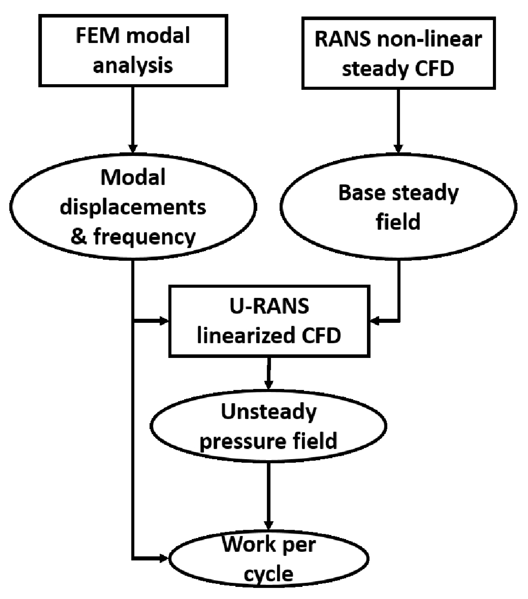
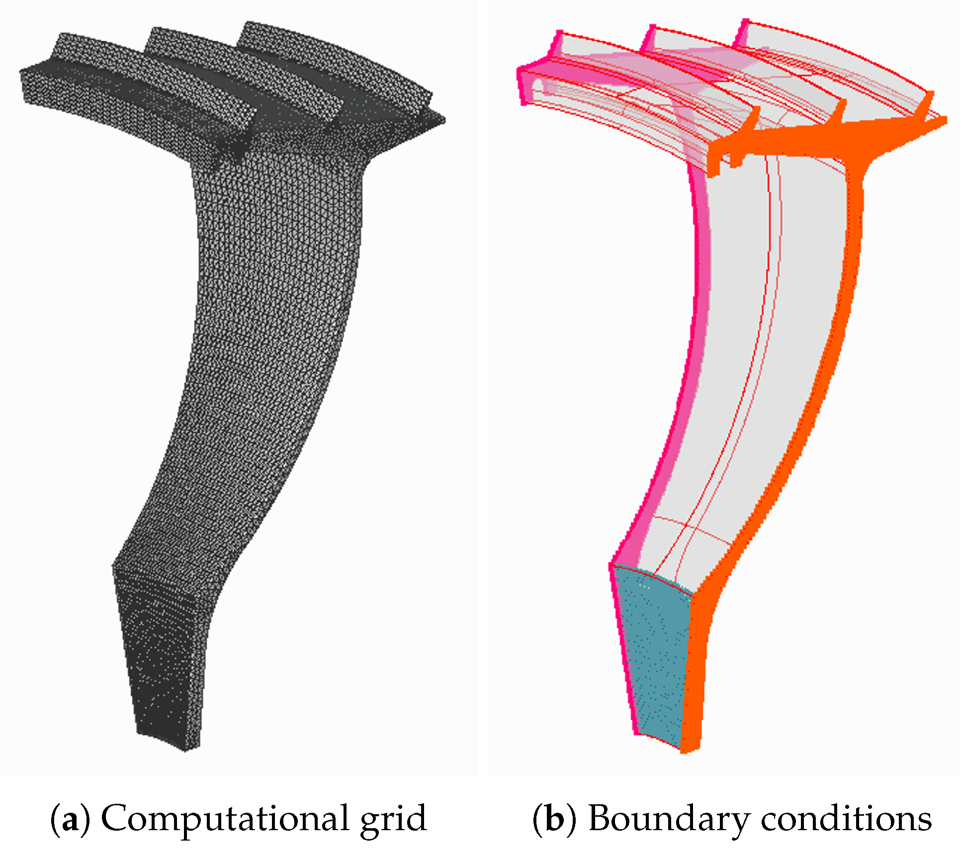
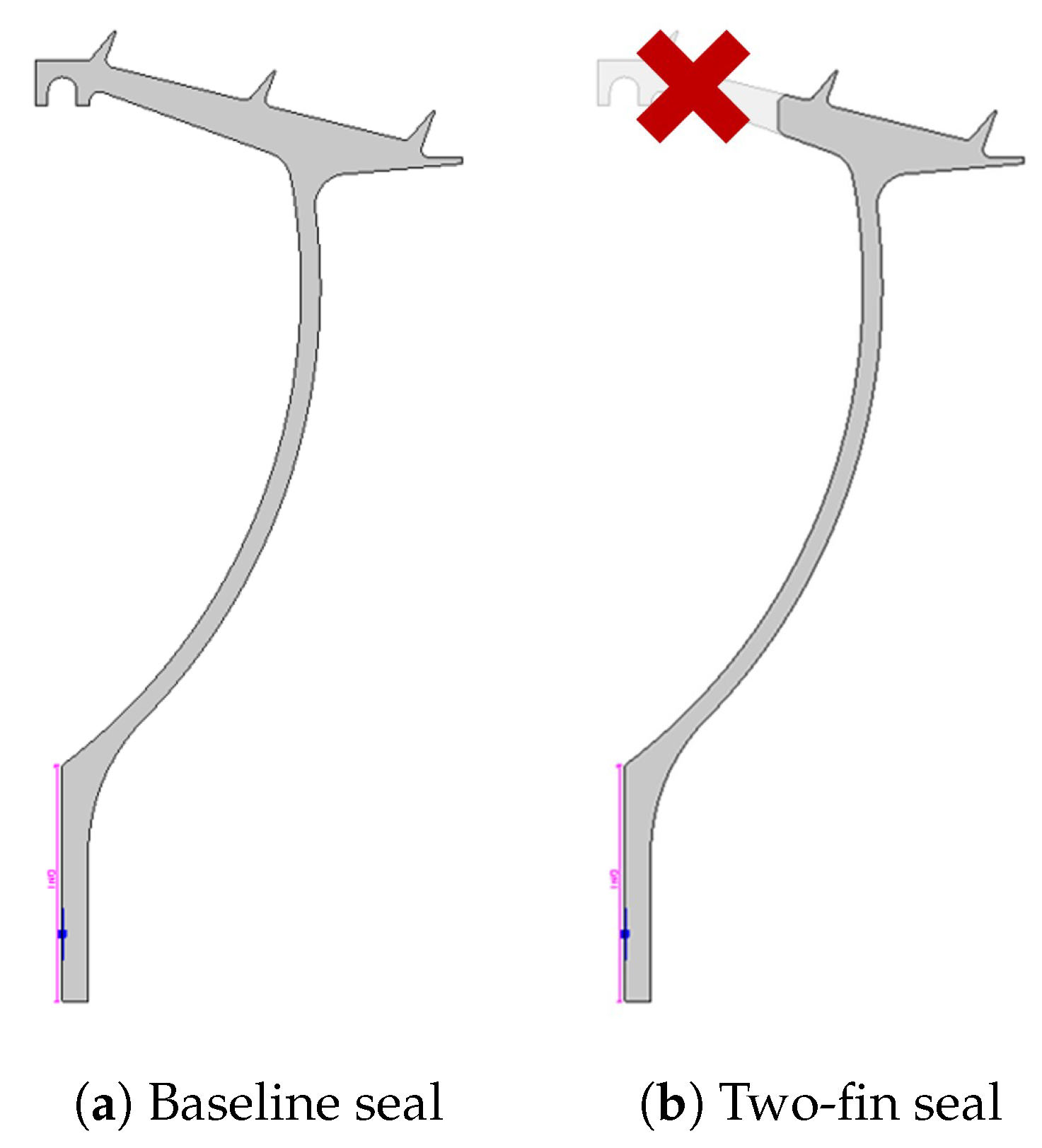
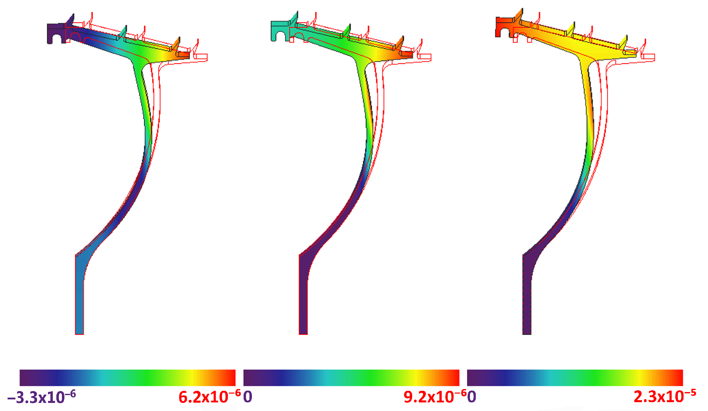
As mentioned in the previous section, the uncoupled methodology requires a modal analysis of the structure to obtain its modal characteristics that will be imposed in the linearised CFD simulation. The calculation of the modal properties considers the static deformation of the seal due to rotational speed and pressure loads through a pre-stress term. Figure 7 illustrates the static deflection of the baseline seal operating at a different shaft speed. Some interesting conclusions can be drawn. Given the position of the pivot point, pressure loads tend to close the right-most clearance while opening the left-most one (0 rpm case). In contrast, centrifugal forces tend to close all the gaps, given that the effect is stronger in the fins at a higher radial position. The relative strength between both effects at the different shaft speeds produces qualitatively different cases, with the maximum closure moving from the right-most to the left-most fin. For the two-fin seal, the behaviour is simpler as both the pressure loads and centrifugal forces tend to reduce the clearances.

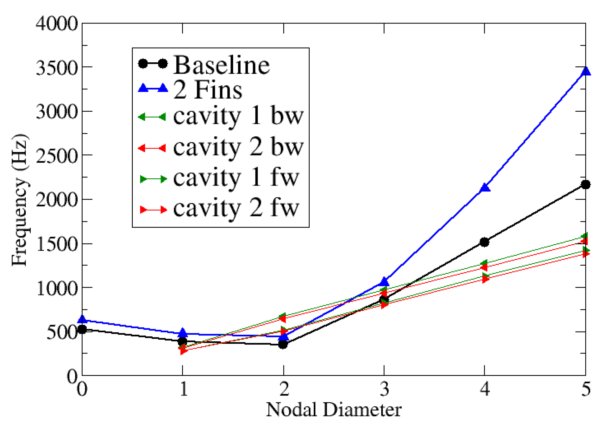
Regarding the calculated modal properties, Figure 8 plots the modal frequencies of the two specimens along with the acoustic frequencies of the seal cavities, both the forwards and backwards travelling waves. The numeration of the inter-fin cavities follows the flow direction from right (HPS) to left (LPS). Focusing on the vibration frequencies, the two-fin seal exhibits higher frequencies than the baseline configuration, mainly due to its lower mass at the fin head. The other characteristic that should be pointed out is the trend of the curves. As the reader can observe, the behaviour of the frequency against the nodal diameter is very similar to that found in disk modes, which should not be a surprise given the kind of structure we are analysing. It is well known that increasing the nodal diameter number imposes more restrictions to the disk displacements, which in turn produce a stiffening effect in the structure and an increase in the natural frequencies. It has to be mentioned that measured instabilities show discrepancies of 2–3% in frequency when compared with the predicted values, which is considered acceptable.

However, the key information from Figure 8 is the ratio between vibrational and acoustic frequencies, because this is one of the main parameters that determine the seal stability. At high nodal diameters, the aforementioned stiffening effect rises vibration frequencies above the acoustic ones (NDs 4–5). In contrast, there is an intermediate region where the opposite is true (ND 2).

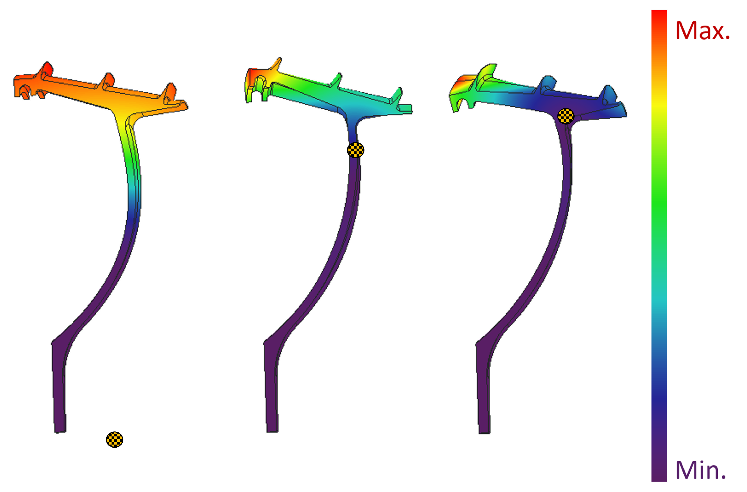
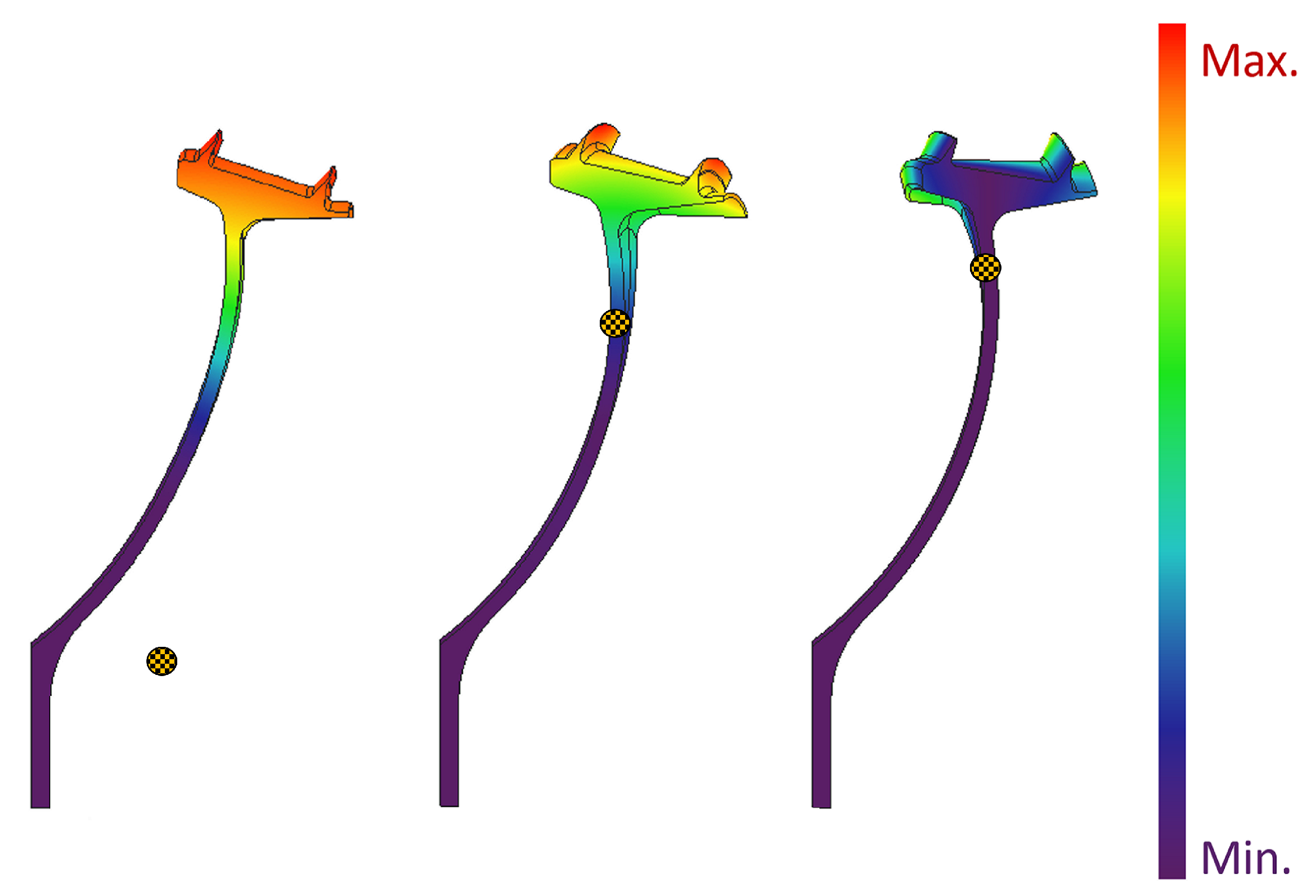
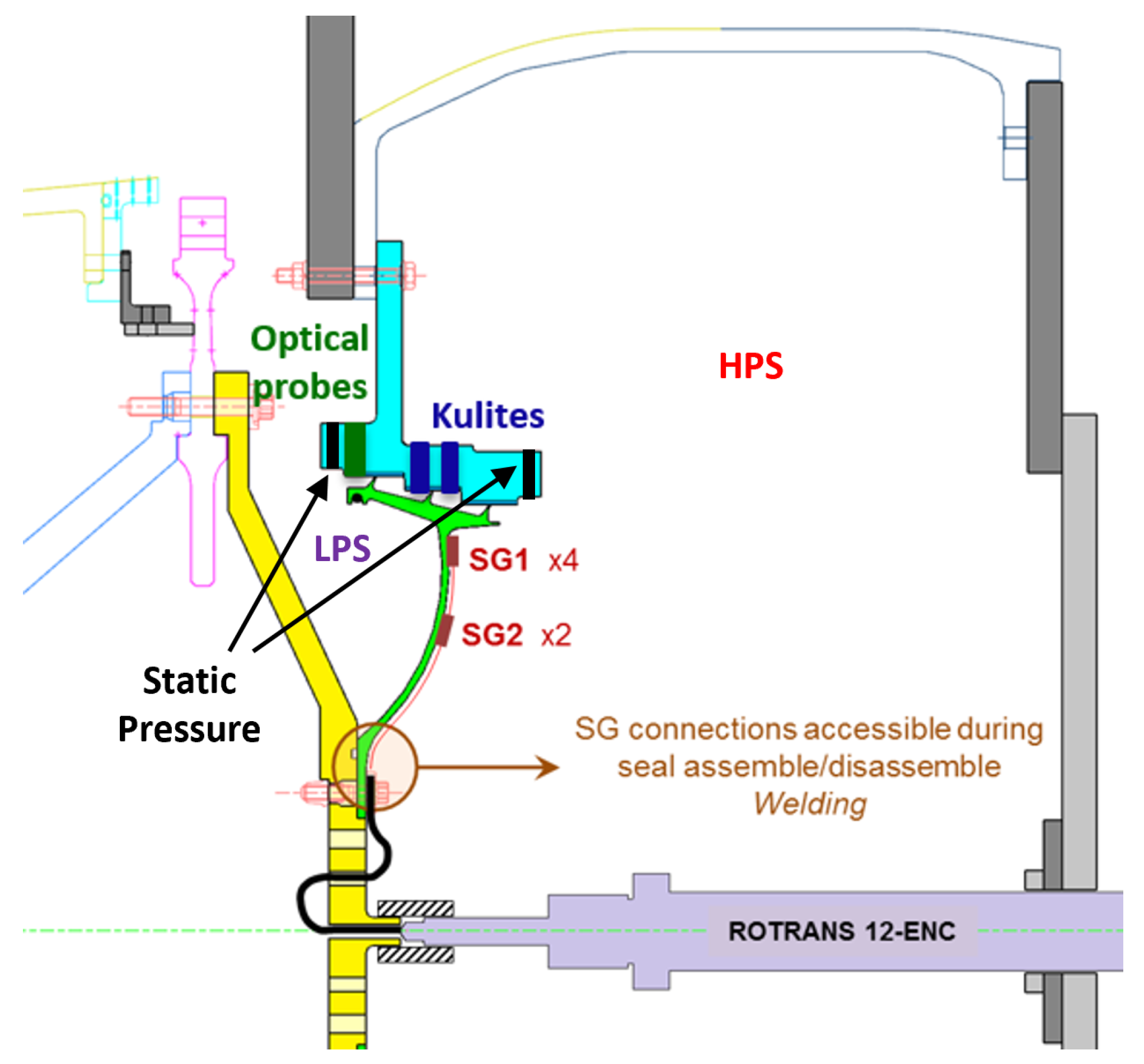
Figure 9 and Figure 10 depict the modal shapes for different nodal diameters with the torsion centre overimposed. The position of the torsion centre is of paramount importance when determining the seal stability. In our case, as we are examining the stability of inclined seals, both the radial and axial coordinates of the pivot point should be considered [8]. We can observe that the torsion centre moves from a position close to the root of the seal to a position close to the joint between the seal head and arm. Consequently, mode shapes evolve from a pure edgewise movement to a torsion mode. According to the axial position of its torsion centre, the baseline geometry is a high-pressure-supported seal (HPS), that is, the torsion centre lies closer to the high-pressure side (right-most side in our case, as depicted in Figure 1). In contrast, the two-fin seal is a low-pressure-supported seal (LPS). However, the axial or edge-wise modal component is comparatively higher in this second seal (note the radial position of the torsion centre in Figure 10), making it difficult to foresee whether it will behave as a LPS or HPS seal.

4.2. Steady Flow

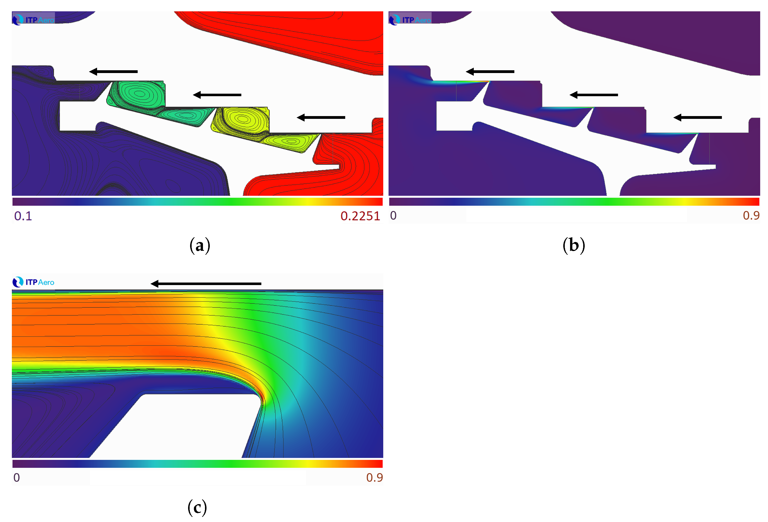
The steady flow in labyrinth seals exhibits a very complex structure with different vortices filling the cavities. Despite this complexity, there are two main regions to consider as depicted in Figure 11:

• The flow inside the cavities (both inner seal cavities and outer cavities) is a low velocity flow. Ignoring the swirl, the meridional Mach number is approximately 0.1 in that region. The static pressure is roughly uniform inside each of the cavities.
• The flow in the tip gaps has a much higher Mach number, with the last (left-most) fin being essentially choked in most operation points. This is the region responsible for most of the pressure losses in the seal.
• A remarkable feature of the flow in the tip gaps is the re-circulation bubble that often appears. This bubble varies in size depending on the operation point but usually affects a significant part (around 25%) of the gap. In practice, this leads to a significant reduction in the effective gap, leading to smaller mass flow through the seal than could be expected from the nominal gap under ideal conditions.

Such characteristics make the CFD simulations more challenging than in other turbine elements such as the blades. The extremely different length and time scales associated with the gaps and cavities regions are not the ideal conditions for numerical codes. Moreover, boundary layers in the fin gaps should be well captured due to its relevance in the results (i.e., re-circulation bubble size and mass flow), imposing severe restrictions to the mesh in the region. Finally, convergence in the low-speed regions of the external cavities can be slow, especially for the thermal part of the problem, making it advisable to use an initial solution with a reasonable temperature field.

When comparing the measurements obtained in the experimental campaign with the predictions obtained with the aforementioned methodology, non-negligible discrepancies may be found (see

Table 2. Discrepancies between CFD steady simulations (nominal gaps of 0.3 mm) and experimental data.

Configuration	$\mathbf{\Omega }$ (r.p.m.)	$\Delta$P (MPa)	$\dot{\mathit{m}}$ Err.	${\mathit{P}}_1$ Err.	${\mathit{P}}_2$ Err.
Baseline	0	0.1674	−23.18%	3.31%	9.81%
	1500	0.1513	−22.46%	3.56%	10.6%
	2200	0.1392	−20.71%	3.44%	9.80%
	2900	0.1251	−18.37%	2.68%	8.11%
2 Fins	0	0.1059	−2.95%	−1.14%	-
	1500	0.0968	19.61%	−0.89%	-
	2200	0.1037	−3.21%	−3.9%	-
	2900	0.1081	−0.55%	−2.22%	-

). There are several possible sources for these discrepancies:

• Deformation of the rotating seal due to the steady loading, including centrifugal forces and pressure differences. Note that our CFD simulations considered the nominal geometry of the seal, that is, static deformation was not included.
• Manufacturing and/or positioning tolerances changing the gap value from the nominal one.
• Mismatch between the CFD predictions and the real flow structure. RANS simulations are inherently limited when dealing with complex flows, and even small errors in the prediction of the size of the re-circulation bubble at the fin tips or the turbulent viscosity in that region can significantly affect the mass flow prediction.
• Rubbing or contact between the rotating seal and the stator, which can cause damage both parts and increase the gaps.

In our case, static deformations obtained from the FEM analysis are small (less than 10% of the total gap) and their impact on the steady field is limited. Moreover, as illustrated in Figure 7, the static deformation tends to close the fin clearances in most of the cases analysed, with the single exception of the 0 rpm case for the baseline configuration in which the left-most fin is opening. Therefore, including the effect in the CFD model would further degrade the matching between simulations and experimental data. Another remarkable point is that the discrepancies found depend on the operating point, which makes us think that the term associated with the CFD (RANS) limitations when calculating the re-circulation bubble has a non-negligible importance, at least as important as manufacturing or assembling tolerances. However, that term alone does not justify differences of up to 20% in mass flow and does not explain why those differences are much smaller for the two-fin seal.

Having said that, the only explanation left is the rubbing. There was evidence of rubbing appearing during the tests leading to a gap widening, which will perfectly explain why the experimental mass flow was higher than that calculated by the CFD. Another interesting point is that as both static and dynamic displacements are higher for the baseline geometry than for the 2-fin seal, it is fair to think that contacts will be more severe in the former, explaining why we are not finding the same level of discrepancies for both seals. However, although rubbing was detected, it was not quantified how much it affected the gaps, which did not allow us to use that information to correctly model the actual geometry in our simulations.

At this point, a different approach had to be followed. Instead of imposing the radial gaps, which essentially were unknown due to the contacts between rotor and stator, it makes sense to try to impose the pressure and mass flow as measured and then develop a numerical procedure to adjust the gaps in order to match those steady magnitudes in our CFD. It consisted of a Newton–Raphson iterative method using numerical differentiation to obtain the Jacobian. For a seal with “N” fins, the system of equations to be solved imply “N-1” equations corresponding to the “N-1” cavities pressure, plus an additional equation corresponding to the mass flow, with “N” gap unknowns (see Equations (2) and (3)):

$$\sum \frac{\partial P_j}{\partial g_i}\Delta g_i=\Delta P_j$$

(2)

$$\sum \frac{\partial \dot{m}}{\partial g_i}\Delta g_i=\Delta \dot{m}$$

(3)

The different partial derivatives are calculated using numerical differentiation by means of CFD simulations with individually modified gaps (+10% in concrete). Additionally, a simulation where all the fin gaps are uniformly modified allows us to calculate the required uniform $\Delta g$ that would yield the experimental mass flow. Taking these new gaps as a reference, the right-hand side of Equation (3) is zero, which simplifies the resolution of the system. The calculated $\Delta g_i$ will then be applied to these new reference gaps, not the nominal ones, yielding the final resulting gaps. The process should be repeated until the desired convergence level is reached. In practice, in most cases, the results were acceptable after a single iteration. The obtained errors both in pressures and mass flow are shown in

Table 3. Discrepancies between CFD steady simulations (adjusted gaps) and experimental data.

Configuration	$\mathbf{\Omega }$ (r.p.m.)	$\Delta$P (MPa)	$\dot{\mathit{m}}$ Err.	${\mathit{P}}_1$ Err.	${\mathit{P}}_2$ Err.
Baseline	0	0.1674	−1.58%	0.42%	−2.44 %
	1500	0.1513	−1.89%	0.16%	−2.23 %
	2200	0.1392	−0.32%	−0.03%	−2.40 %
	2900	0.1251	2.37%	−0.61%	−2.98 %
2 Fins	0	0.1059	−0.10%	0.07%	-
	1500	0.0968	−0.37%	0.37%	-
	2200	0.1037	−0.57%	0.03%	-
	2900	0.1081	−0.06%	0.08%	-

.

4.3. Unsteady Flow Field

In this section, we will focus on the unsteady pressure field obtained from the linearised unsteady problem. Figure 12a,b show that most of the activity is located at the inter-fin cavities, being the dominant term of the problem. The result is not surprising considering that pressure variations in the cavities occur due to volume and mass flow changes. These two terms should be negligible in the outer cavities given their size. However, as we will see later, the outer cavities may exhibit high unsteady pressure levels under certain operating conditions.

Another distinctive feature of the obtained unsteady pressure field is its uniformity inside each of the inter-fin cavities. As expected, the cavity positioned further from the pivot point (left-most cavity) presents higher pressure levels. However, when we increase the ND number and frequencies rise (see Figure 8), the uniformity of the pressure field breaks. The main reason behind this effect is the excitation of high-mode acoustic resonances of the inter-fin cavities. In our case, the effect becomes apparent for ND +5 (see Figure 12b).

Finally, we would like to highlight that the unsteady pressure values obtained are dependent on the movement amplitude imposed in the simulation. In our simulations, the resulting unsteady pressure levels (Figure 12) are two orders of magnitude lower than the corresponding steady pressure values (Figure 11). This is consistent with the linearity hypothesis employed in our methodology.

4.4. Seal Stability

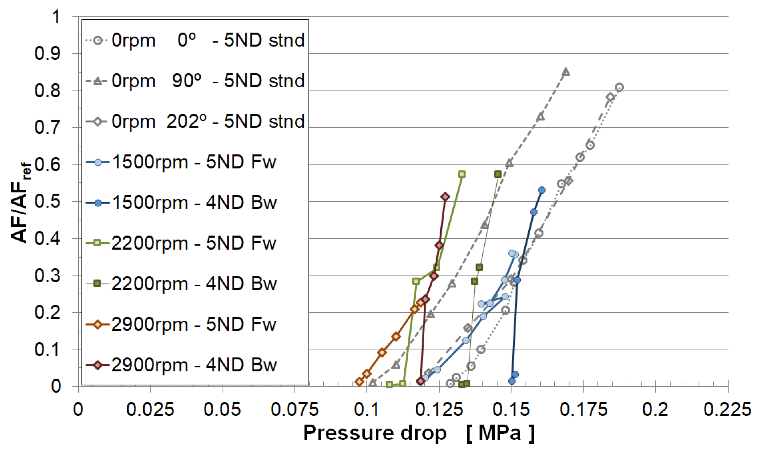
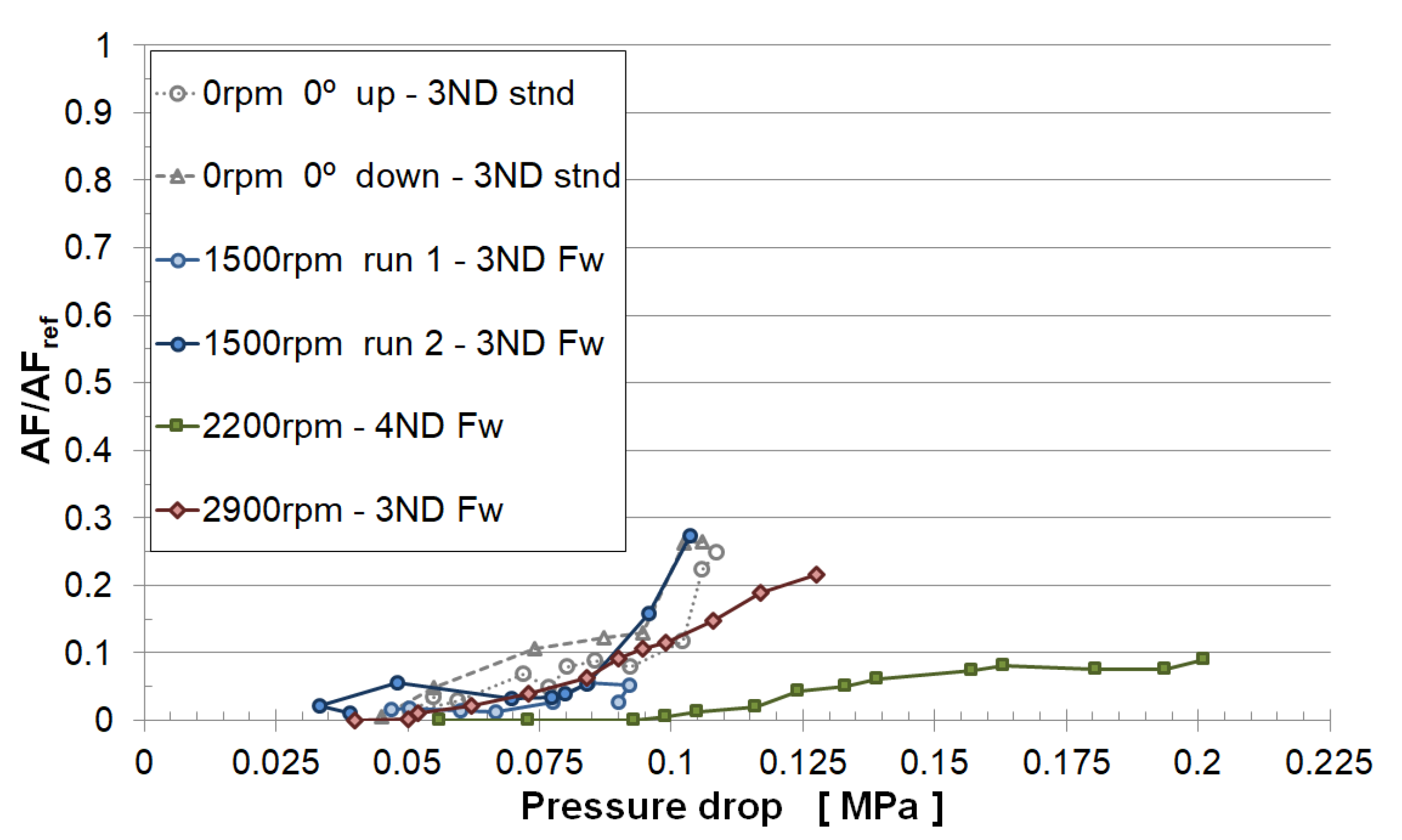
The experimental measurements corresponding to the baseline and two-fin specimens are plotted in Figure 13 and Figure 14, respectively. In concrete, these graphs plot the vibration amplitude–frequency parameter (AF) as a function of the pressure drop across the seal. Note that AF values have been normalised with the maximum AF measured in all the campaign, using that same reference value in all of the plots. Each line represents the different nodal diameters detected, discerning between standing waves (stnd) and forwards (Fw) or backwards (Bw) travelling waves.

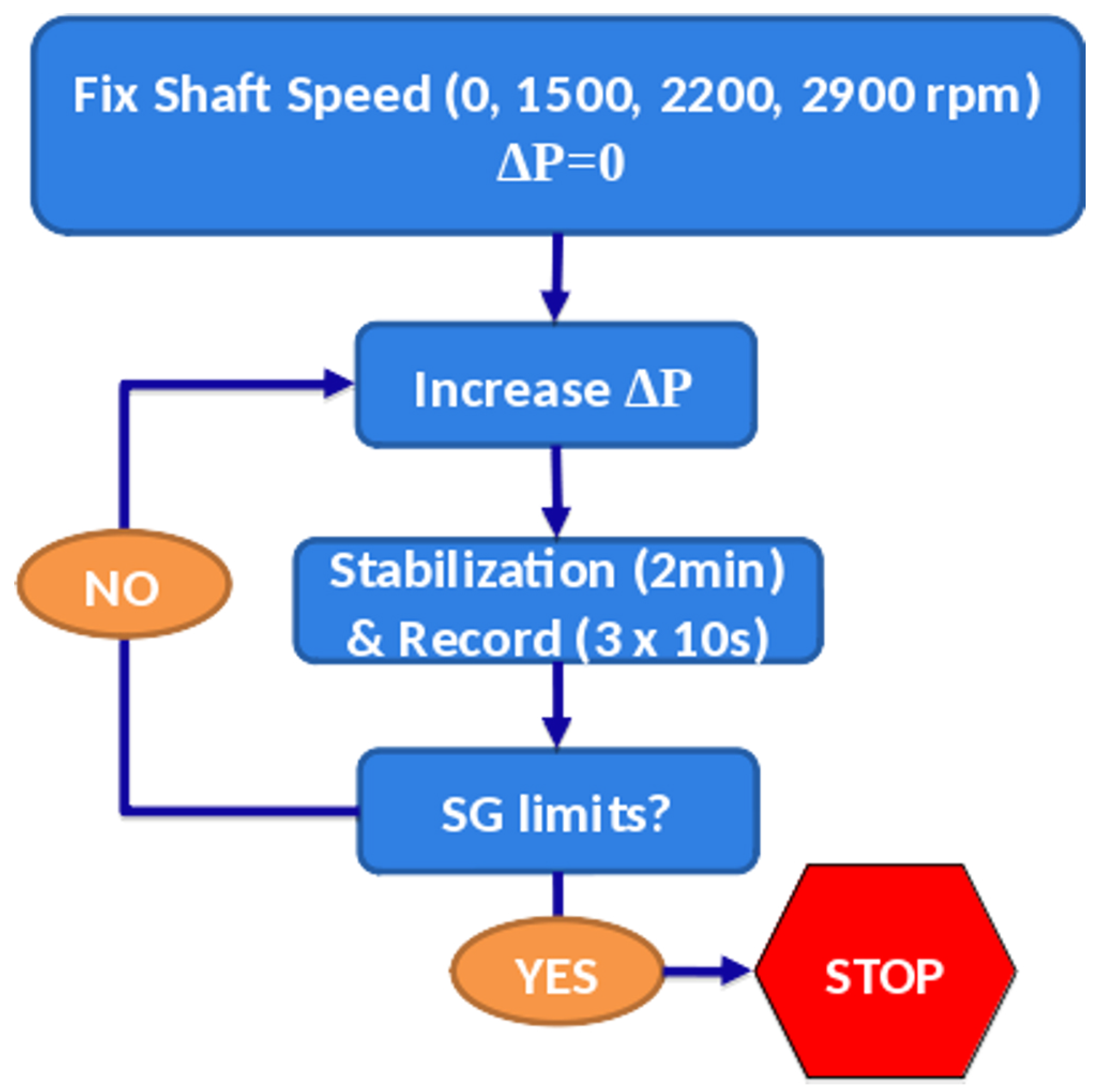
The most remarkable outcome from the experiments is that all of the specimens experimented flutter at every rotational speed tested. Depending on the seal specimen and rotational speed chosen, the minimum pressure drop required to initiate the instability was different. Once flutter appeared, the vibration amplitude could grow really fast as results plotted in Figure 13 show, underlining the importance of a good control system to allow an easy, fast and safe termination of the test.

Comparing results between the baseline and two-fin geometries (Figure 13 and Figure 14), two main differences can be found. First, the two-fin seal becomes more unstable at lower pressure ratios than the baseline specimen does, that is, it reaches its unstable region before; second, the vibration amplitudes rise more abruptly in the baseline case, implying a higher absolute aerodynamic damping level (this point is confirmed by CFD simulations, see Figure 15). Summarising, the two-fin seal reaches its unstable region first, but once we enter that region, the instability itself is less severe than that observed in the baseline configuration.

Both points can be easily related to the modal shapes and frequencies of both seals. Regarding the modal shape or torsion centre position, the baseline seal can be considered as a HPS seal, while the two-fin seal is an LPS seal (see Figure 9 and Figure 10). However, the two-fin seal behaves in the opposite sense as a combination of being inclined and having relatively high axial displacements when compared to the radial ones (note the radial position of the corresponding torsion centre in Figure 10). The Corral–Vega model for stepped seals [8] covers this fact. Thus, as both seals behave as HPS-supported seals, the one with the higher frequency will be the one closer to the unstable region, according to Abbot’s criteria. As it was mentioned before, Figure 8 shows that effectively, the two-fin seal is the one with higher modal frequencies.

Finally, regarding the absolute value of the damping itself, it should be taken into account that the baseline configuration has an additional cavity positioned further from the pivot point, thus producing higher unsteady pressure levels and work per cycle. In fact, in the two-fin seal specimen, the pivot point lies somewhere in between the two fins, splitting the inter-fin cavity into two regions that will produce works per cycle with the opposite sign, reducing its capability to produce high levels of aerodynamic damping.

Before showing the stability results from the CFD simulations, a couple of clarifications should be made. The first thing to consider is that our simulations do not include any mechanical damping and do not attempt to calculate any vibration amplitude. That kind of study is beyond the scope of this paper. The target of our analysis is to determine whether the seal is aerodynamically unstable when operating at a given condition. This is a necessary but not sufficient condition to have flutter, as mechanical friction could prevent vibration depending on the relative importance of both terms. In addition, when more than a single unstable nodal diameter coexists, the most unstable one (after considering the mechanical damping) tends to prevail. With that in mind, it is not a surprise that simulations predict a wider set of unstable nodal diameters than those detected by the experimental readings. The only thing that can be demanded to simulations of the kind presented here is that the experimentally measured nodal diameters are among the predicted set of unstable ones.

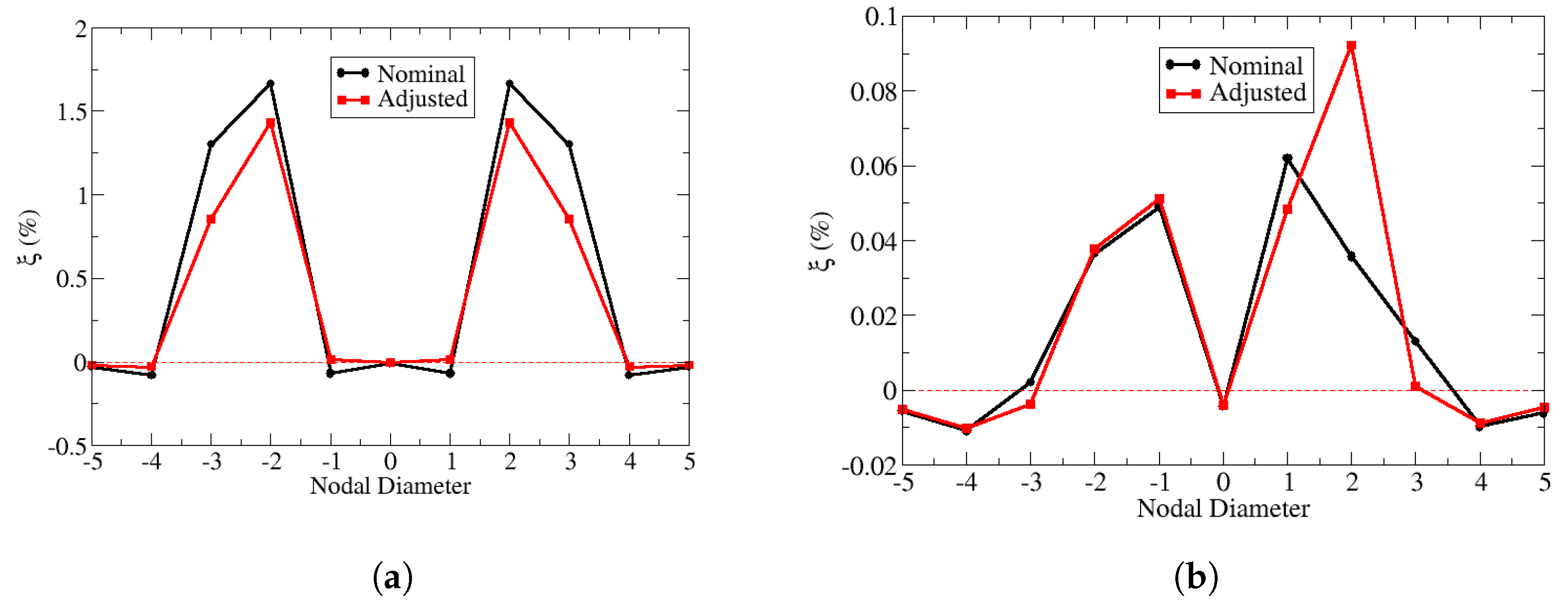
Figure 15 depicts the impact of the adjusted clearances on the aerodynamic damping both for the baseline and two-fin geometries. It is remarkable how the effect can modify the sign of the damping for some nodal diameters, that is, its stability. The influence of the fin gaps over the aerodynamic damping comes from both the steady and unsteady flow fields modification. Generally, equally closing the gaps tends to destabilise the seal. However, when the seal exhibits dissimilar clearances (as it happens in our adjusted gaps case and in real operation), the behaviour is complex and difficult to predict in advance [18].

Table 4. Flutter instabilities of the baseline configuration from simplified domain simulations. Results with nominal and adjusted gaps.

Ω (r.p.m.)	ΔP (MPa)	Experimental	CFD (Nominal)	CFD (Adjusted)
0	0.1674	ND ± 5	ND 0, ±1, ±4, ±5	ND 0, ±4, ±5
1500	0.1513	ND + 4, −5	ND 0, ±1, ±4, ±5	ND 0, −1, ±4, ±5
2200	0.1392	ND + 4, −5	ND 0, −1, ±4, ±5	ND 0, −1, ±4, ±5
2900	0.1251	ND + 4, −5	ND 0, −1, ±4, ±5	ND − 1, −4, ±5

and

Table 5. Flutter instabilities of the 2-fin configuration from simplified domain simulations. Results with nominal and adjusted gaps.

Ω (r.p.m.)	ΔP (MPa)	Experimental	CFD (Nominal)	CFD (Adjusted)
0	0.1059	ND ± 3	ND 0, ±4, ±5	ND 0, ±4, ±5
1500	0.0968	ND − 3	ND 0, ±4, ±5	ND 0, −3, ±4, ±5
2200	0.1037	ND − 4	ND 0, +3, ±4, ±5	ND 0, +3, ±4, ±5
2900	0.1081	ND − 3	ND 0, +3, ±4, ±5	ND 0, +3, ±4, ±5

summarise the results for all operating conditions. The first point to highlight is that both geometries have been predicted as unstable (negative aerodynamic damping) for all the shaft speeds, as it happened in the testing campaign. However, the predicted instabilities are only in moderate agreement with the experiments. Regarding the baseline geometry, the nominal gaps simulation correctly predicted all the instabilities; although, the adjustment procedure modifies the results reducing the list of unstable nodal diameters. Note that, for the 2900 rpm case, the simulations with adjusted gaps predict a stabilization of ND + 4, which was the one observed in the experiments. A deeper analysis indicates that ND + 4 (backwards wave) is operating in a region close to the stability limit. This region is really sensitive to details, with minor changes in the involved parameters producing big changes in damping values, both in sign and magnitude, and thus, it is hard to predict by the simulations. For instance, the uncertainties regarding the actual gap values in the experiments could explain the difference.

In contrast, the two-fin specimen simulations do not match the experimental measurements so well, failing to predict the 0 rpm case and not capturing the travelling wave sign in the 2900 rpm case. It should be mentioned that the instability at 1500 rpm (ND − 3) is well captured only after the gap-adjustment process takes place, even though the gap correction for the two-fin geometry was not too big. This fact emphasises the necessity to feed the simulations with the right gap values.

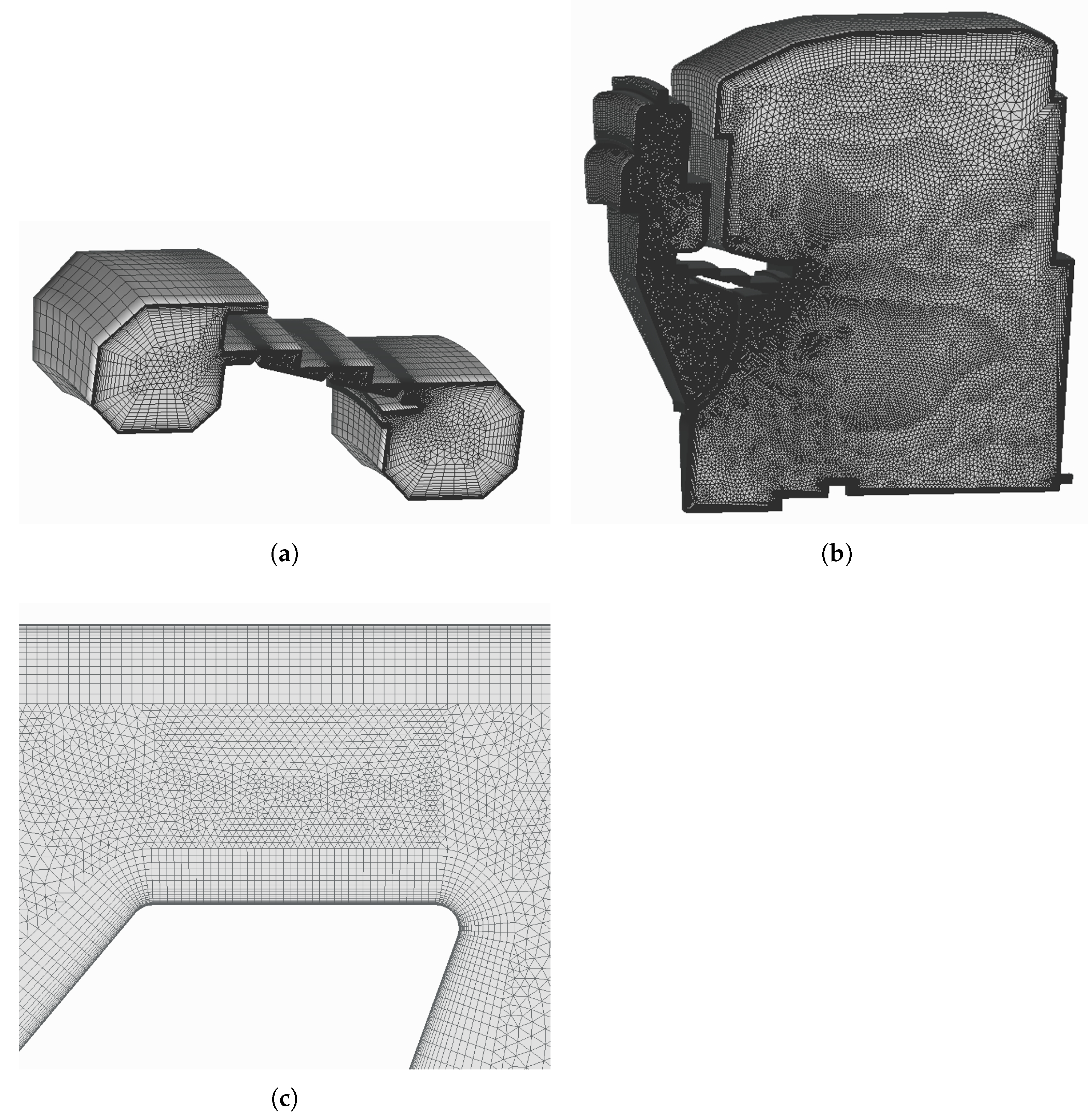
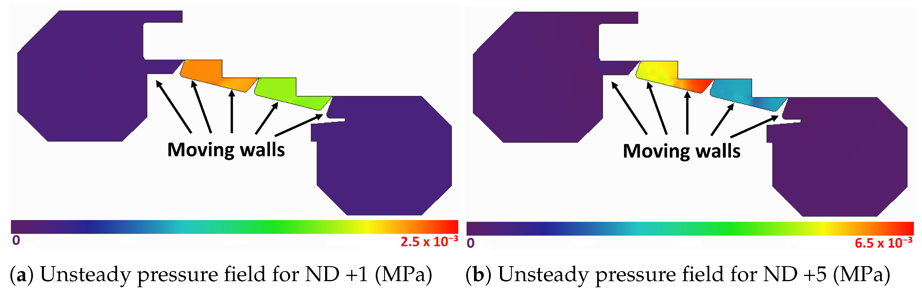
All the results shown so far correspond to the simulations performed with the simplified domain (see Figure 6). By simplifying the domain, we intend to reduce the computational cost, but at the same time, we are neglecting the effect of outer cavities in the overall stability of the seal. Although this is essentially true in most cases, as unsteady pressure plots in Figure 12 show, external cavities may play a non-negligible role regarding stability under certain circumstances. When vibration frequencies approach the natural frequencies of those cavities, a resonance occurs and noticeably unsteady pressure levels may appear. Moreover, that pressure will act over a wide seal surface, thus having the potential to become the dominant term of the problem. Keeping that in mind, additional simulations using the full domain have been run. This domain incorporates the whole seal structure along with the actual geometry of the external cavities (see Figure 6).

Before going on to comment on the stability changes observed in these additional simulations, it is worth mentioning that the steady state remains almost unaffected, and so previously shown results and discussion regarding the steady results still applies. Having said that, the first thing we observe in the unsteady linearised problem solutions is that CFD confirms that the seal vibration is exciting the outer cavities resonances for some nodal diameters, as Figure 16 shows. 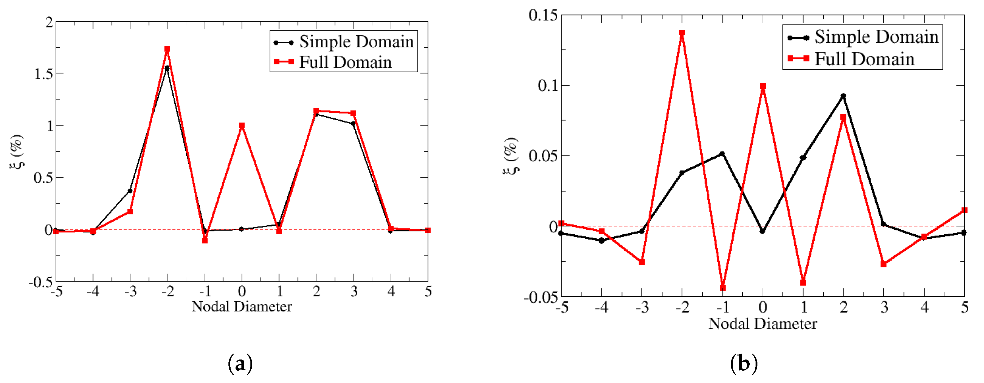Figure 17 gives a closer look at the effect, comparing the resulting aerodynamic damping curves with and without the external cavities contribution. It can be clearly seen that nodal diameter 0 is stabilised by the external cavity resonance in both configurations. For the baseline configuration, the effect is weak apart from the ND 0 resonance, as expected. In contrast, the same can not be said for the two-fin configuration. As mentioned before, the aerodynamic damping produced by this seal is low when compared to the baseline case. Therefore, it is easier for the external cavities to modify the seal stability, even when no external resonance is being excited.

Table 6. Flutter instabilities for the baseline configuration from full domain simulations with adjusted gaps.

Ω (r.p.m.)	ΔP (MPa)	Experimental	CFD (Adjusted Gaps)
0	0.1674	ND ±5	ND ±1, ±5
1500	0.1513	ND + 4, −5	ND ±1, −4, ±5
2200	0.1392	ND + 4, −5	ND −1, ±4, −5
2900	0.1251	ND + 4, −5	ND −1, −3, −4, −5

and

Table 7. Flutter instabilities for the 2-fin configuration from full domain simulations with adjusted gaps.

Ω (r.p.m.)	ΔP (MPa)	Experimental	CFD (Adjusted Gaps)
0	0.1059	ND ±3	ND ±1, ±3
1500	0.0968	ND − 3	ND ±1, ±3, ±4
2200	0.1037	ND − 4	ND ±1, ±3, −4
2900	0.1081	ND − 3	ND ±1, ±3, −4

summarise the stability results from the CFD simulations including the external cavities.

Regarding the agreement between simulations and experimental stability, we must highlight that the new results obtained for the two-fin geometry (shown in Table 7) perfectly match the experiments in all the operating points analysed. However, for the baseline configuration we obtain mixed results; while we are improving the matching in some aspects, (ND 4 is not predicted as unstable at 0 rpm or ND 5 instability is reduced to the forwards travelling wave at 2200 and 2900 rpm, in line with the tests) it seems we are over predicting the effect of external cavities over the ND 4 backwards travelling wave, which suffers a complete stabilization at 1500 rpm (see Figure 17a), in contrast with the experimental data. Here, the same comments as before apply. The ND + 4 is close to the stability limit (i.e., aerodynamic damping 0) and in an operating region really sensible to details. Therefore, it is hard to predict by the simulations.

Overall, we think the agreement between the detailed simulations (i.e., adjusted gaps and full domain) and experimental data is really good, only failing to predict the aforementioned travelling wave sign of ND 4 instability in the baseline configuration.

5. Conclusions

The stability of two realistic labyrinth seal geometries has been analysed with an FEM-CFD uncoupled linear methodology, and the results obtained have been compared with existing experimental data. The nature of the typical flow through labyrinth seals represented a challenge for the numerical code, both from the accuracy and convergence points of view. In addition, the uncertainties regarding actual gap values during testing complicated the modelling of the problem even more.

Despite that, the agreement between simulations and test data is considered reasonably good after applying the gaps adjustment process and including the external cavities, which proved to have a non-negligible impact on the seal stability, especially for the two-fin seal. Thus, we consider the validity of the proposed methodology is confirmed by the obtained results.

References

1. Lewis, D.; Platt, C.; Smith, E. Aeroelastic instability in F100 labyrinth air seals. J. Aircr. 1979, 16, 484–490. [Google Scholar] [CrossRef]
2. Ehrich, F. Aeroelastic Instability in Labyrinth Seals. J. Eng. Power 1968, 90, 369–374. [Google Scholar] [CrossRef]
3. Alford, J.S. Nature, causes, and prevention of labyrinth air seal failures. J. Aircr. 1975, 12, 313–318. [Google Scholar] [CrossRef]
4. Abbott, D.R. Advances in Labyrinth Seal Aeroelastic Instability Prediction and Prevention. J. Eng. Power 1981, 103, 308–312. [Google Scholar] [CrossRef]
5. di Mare, L.; Imregun, M.; Green, J.S.; Sayma, A.I. A Numerical Study of Labyrinth Seal Flutter. J. Tribol. 2010, 132, 022201. [Google Scholar] [CrossRef]
6. Miura, T.; Sakai, N. Numerical and Experimental Studies of Labyrinth Seal Aeroelastic Instability. J. Eng. Gas Turbines Power 2019, 141, 111005. [Google Scholar] [CrossRef]
7. Corral, R.; Vega, A. Conceptual Flutter Analysis of Labyrinth Seals Using Analytical Models. Part I: Theoretical Support. J. Turbomach. 2018, 140, 121006. [Google Scholar] [CrossRef]
8. Corral, R.; Vega, A.; Greco, M. Conceptual Flutter Analysis of Stepped Labyrinth Seals. J. Eng. Gas Turbines Power 2020, 142, 071001. [Google Scholar] [CrossRef]
9. Corral, R.; Greco, M.; Vega, A. Higher Order Conceptual Model for Labyrinth Seal Flutter. J. Turbomach. 2021, 143, 071006. [Google Scholar] [CrossRef]
10. Corral, R.; Greco, M. Experimental Validation of a Seal Flutter Model. J. Turbomach. 2023, 145, 121010. [Google Scholar] [CrossRef]
11. Corral, R.; Beloki, J.; Calza, P.; Elliott, R. Flutter Generation and Control Using Mistuning in a Turbine Rotating Rig. AIAA J. 2019, 57, 782–795. [Google Scholar] [CrossRef]
12. Corral, R.; Gallardo, J.M.; Vasco, C. Aeroelastic Stability of Welded-in-Pair Low Pressure Turbine Rotor Blades: A Comparative Study Using Linear Methods. J. Turbomach. 2004, 129, 72–83. [Google Scholar] [CrossRef]
13. Cordoba, O. FEM Considerations to Simulate Interlocked Bladed Disks With Lagrange Multipliers. In Proceedings of the Turbo Expo: Power for Land, Sea, and Air, London, UK, 22–26 June 2020; Paper GT2020-15140. Volume 10B, p. V10BT26A009. [Google Scholar] [CrossRef]
14. Corral, R.; Crespo, J.; Gisbert, F. Parallel Multigrid Unstructured Method for the Solution of the Navier–Stokes Equations. In Proceedings of the 42nd AIAA Aerospace Sciences Meeting and Exhibit, Reno, NV, USA, 5–8 January 2004. AIAA Paper 2004-0761. [Google Scholar] [CrossRef]
15. Gisbert, F.; Corral, R.; Pueblas, J. Computation of Turbomachinery Flows with a Parallel Unstructured Mesh Navier–Stokes equations Solver on GPUs. In Proceedings of the 21st AIAA Computational Fluid Dynamics Conference, San Diego, CA, USA, 24–27 June 2013. [Google Scholar] [CrossRef]
16. Tyacke, J.; Jefferson-Loveday, R.; Tucker, P. On LES Methods Applied to Seal Geometries. In Proceedings of the ASME Turbo Expo 2012: Turbine Technical Conference and Exposition, Copenhagen, Denmark, 11–15 June 2012; Volume 8, pp. 2053–2065. [Google Scholar] [CrossRef]
17. Wein, L.; Seume, J.; Schmierer, R.; Herbst, F. Large-Eddy-Simulation of Labyrinth Seal Flows. In Proceedings of the Global Power and Propulsion Society, Chania, Greece, 12–14 September 2022. [Google Scholar] [CrossRef]
18. Corral, R.; Greco, M.; Vega, A. Effective Clearance Furthermore, Differential Gapping Impact on Seal Flutter Modelling and Validation. In Proceedings of the ASME Turbo Expo 2021: Turbomachinery Technical Conference and Exposition, Virtual, 1–7 June 2021; Volume 9A. [Google Scholar] [CrossRef]
Figure 1. Test rig assembly (baseline geometry).
Ijtpp 09 00013 g001
Figure 2. Schematics of testing procedure.
Ijtpp 09 00013 g002
Figure 3. Geometries tested in the E-Break project.
Ijtpp 09 00013 g003
Figure 4. Uncoupled structural-fluid linearised methodology.
Ijtpp 09 00013 g004
Figure 5. FEM model mesh and boundary conditions.
Ijtpp 09 00013 g005
Figure 6. CFD domains and associated grids. (a) Computational mesh for the simplified domain. (b) Computational mesh for the complete domain. (c) Detail of the computational mesh in the fin-clearance region.
Ijtpp 09 00013 g006
Figure 7. Contour of static radial displacements (m) of the baseline geometry. Shaft speed of 0 rpm (left), 1500 rpm (centre) and 2900 rpm (right).
Ijtpp 09 00013 g007
Figure 8. Modal and acoustic frequencies at 1500 rpm.
Ijtpp 09 00013 g008
Figure 9. Contour plot of the modal displacement module for the baseline geometry and torsion centre position. ND 1 (left), ND 3 (centre) and ND 5 (right).
Ijtpp 09 00013 g009
Figure 10. Contour plot of the modal displacement module for the 2-fin geometry and torsion centre position. ND 1 (left), ND 3 (centre) and ND 5 (right).
Ijtpp 09 00013 g010
Figure 11. Steady solution from CFD. Baseline geometry operating at 2900 rpm, ΔP = 0.1251 (MPa). Arrows indicate the flow direction, from right to left. (a) Static pressure (MPa). (b) Mach number. (c) Detail of the left-most (last) fin clearance. Mach number.
Ijtpp 09 00013 g011
Figure 12. Unsteady pressure field (MPa) at inter-fin cavities for the baseline geometry, simplified domain and nominal (0.3 mm) gaps. Operating point: 1500 rpm, ΔP = 0.1513 MPa.
Ijtpp 09 00013 g012
Figure 13. Baseline geometry experimental SG readings (CTA Campaign).
Ijtpp 09 00013 g013
Figure 14. Two-fin geometry experimental SG readings (CTA Campaign).
Ijtpp 09 00013 g014
Figure 15. Fin clearances influence on critical aerodynamic damping ratio. (a) Baseline geometry operating at 0 rpm and ΔP = 0.1674 MPa. (b) Two-fin geometry operating at 1500 rpm and ΔP = 0.0968.
Ijtpp 09 00013 g015
Figure 16. Unsteady pressure in external cavities for ND 0 (MPa).
Ijtpp 09 00013 g016
Figure 17. Influence of external cavities in the critical aerodynamic damping ratio. Simulations with adjusted gaps. (a) Baseline geometry operating at 1500 rpm and ΔP = 0.1513 MPa. (b) Two-fin geometry operating at 1500 rpm and ΔP = 0.0968 MPa.
Ijtpp 09 00013 g017