Data-Driven Anomaly Detection Framework for Complex Degradation Monitoring of Aero-Engine

Abstract

Data analysis is an important part of aero engine health management. In order to complete accurate condition monitoring, it is necessary to establish more effective analysis tools. Therefore, an integrated algorithm library dedicated for engine anomaly detection is established, which is PyPEFD (Python Package for Engine Fault Detection). Different algorithms for baseline modeling, anomaly detection and trend analysis are presented and compared. In this paper, the simulation data are used to verify the function of the anomaly detection algorithms, successfully completing the detection of multiple faults and comparing the accuracy algorithm under different conditions.

1. Introduction

Predictive maintenance mainly addresses the reliability problem of the engine, ensuring that the aero-engine has the ability to operate normally under specified conditions. This is an important prerequisite for aircraft safety, because failures of safety-critical systems such as aircraft engines can cause significant economic disruptions and even major accidents with a potential loss of human lives. Therefore, the prediction of the engine failure is of great importance for maintaining the functionality of safety-critical systems, which puts forward higher requirements for engine performance status monitoring [1,2,3]. The trend within the aerospace maintenance industry is searching for new technologies, such as predictive maintenance systems based on health monitoring, to detect degradation earlier and proactively schedule maintenance activities in order to reduce the unscheduled maintenance events. Therefore, the prediction of the engines failure is of great importance for maintaining the functionality of safety-critical systems, which puts forward higher requirements for engine performance status monitoring [4].

Advanced sensor technology has led to the development of condition monitoring technologies. For industrial applications, the frontier issue of multi-modal data analysis should be the combination of applicable data mining methods [5]. Nowadays, data-driven techniques have been reported in the literature for health monitoring of gas turbine engines. Those algorithms can be divided into classification, clustering, regression, dimensionality reduction, etc. William R. et al. proposed a fault detection framework, combining Gaussian mixture model and Hidden Markov model to perform state determination of VSVA (variable stator vane actuator) system used in aero-engine [6]; Consumi et al. established a Bayesian inference method to execute turbojet engines gas path analysis [7]. The Cluster AD-Flight clustering model proposed by Li L uses the DBSCAN (Density-Based Spatial Clustering of Applications with Noise) algorithm for multi-dimensional clustering analysis to exclude abnormal flight from multiple nominal patterns in takeoff phase [8]. Regression-based methods are also widely used. These methods use regression models to fit multi-dimensional data, and then detect abnormalities based on the predictions of the regression models and the differences in data observations. Dewallef P et al. adapted Kalman filter model to deal with the performance monitoring and fault diagnosis problems based on several gas path measurements, including fuel flow, spool speed and the temperature of compressor blade and casing [9]; Seo D H et al. proposed a neural network framework fusing with support vector machine to monitor engine’s working state, and the framework has been applied to the on-design and off-design performance data of a turbo-shaft engine have been generated by the gas turbine simulation program (GSP) [10].

Another topic related to anomaly detection is the neighborhood-based method. It selects a distance or use a similarity measurement method to define a neighborhood, and calculates the distance or relative density between a sample point and its neighborhood as an anomaly score. In this field, Puranik et al. applied both k-nearest neighborhood (KNN) and local outlier factor (LOF) to conduct quantitative analysis of flight data outlier detection [11]. Another KNN method used for data anomaly detection is carried out by Manukyan A et al. aiming at detecting instantaneous abnormal points [12].

However, the development process of anomaly detection algorithm for engine’s data reflects several problems. First, very few public data sets to obtain. Algorithm development requires data sets, especially fault data for verification, while the real engine data is difficult to obtain due to confidentiality issues, and the number of faults contained is very rare. Moreover, engine data usually involves technical secrets and cannot be easily released [13]. Second, although there are many algorithms, only part of them is suitable for engine detection, that is, lacking an integrated detection algorithm library. The complete engine monitoring process includes baseline construction, anomaly detection and trend prediction, and this requires multiple algorithms’ cooperation. Lastly, too many applications of classic machine learning algorithms, and lack of some attempts to apply new algorithms in the field of artificial intelligence for engine condition monitoring [14].

This paper has been divided into five sections. Section 2 introduces the engine condition monitoring data and enumerates its particularity. Section 3 enlists the machine learning techniques in the developed algorithm toolbox for engine anomaly detection. Section 4 includes detailed description of the simulation data set of engine gas path faults and the comparison of the detection results using the various algorithm of the developed toolbox. Finally, Section 5 concludes the work.

2. Commercial Aircraft Engine Condition Monitoring

2.1. Engine Gas Path Analysis

The performance of aero-engines is referred to the carefully tuned interaction among each gas path component. The high-pressure compressor (HPC) and high-pressure turbine (HPT) is often referred to as the core engine, which is in charge of generating power that the LPT uses to transform into mechanical power for driving the fan. Typical sensors in aero-engine system include temperature sensors, speed sensors and pressure sensors located in different stations of engine. These raw sensor data contain control and feedback mechanisms; thus, simple analysis cannot obtain effective degradation information. Other condition parameters, such as Mach number, altitude and atmospheric temperature are included for further analysis. Figure 1 shows the online built-in sensor parameters of a typical modern turbofan engine, covering the main gas path components of the engine and important accessory systems (accessory systems such as lubricating oil and fuel control), etc. [15].

Gas path analysis (GPA) is a method that relates variations of measured engine performance parameters resulting from engine deterioration to the condition of its gas path components [16]. It is meaningful to the existing gas turbine diagnostic methods, which is wildly used for condition-based maintenance. In order to put these methods into practical applications, improving diagnostic accuracy has been the focal point for developing better GPA techniques [17,18,19].

Existing approaches can be grouped in two categories: physics-based methods and data-driven methods. The physics-based methods aim at describing the physics of failure mechanisms by mathematical modeling for the components and the systems under the study. Such methods are applicable where there is enough information about the internal parameters of the system and the failure mechanisms can be parameterized on that basis. Houman Hanachi et al. developed a robust physics-based performance indicator for aero-engine [20]. A comprehensive physics-based thermodynamic model for the gas path of a single shaft engine was developed in their work to accurately predict the cycle parameters based on limited actual operating data. Physical degradation processes are only well understood for critical or relatively simple components, and physics-based approaches are generally hindered by their limited ability to properly tune the parameters of models with high complexity or model incompleteness, which restricts the deployment in practical applications [21]. The alternative approach for health monitoring is the use of data-driven models [22]. These approaches use large amounts of data, preferably from various sources, and apply data analytics techniques such as machine learning and artificial neural networks to discover patterns and relations in the data sets. This means that in principle no knowledge on the system characteristics or failure behavior is required, which makes the approach popular and widely accessible [23].

2.2. Engine Condition Monitoring Data

A flight is divided into different flight phases, each phase has a different impact on the engine, which increases the difficulty of data monitoring. Currently, Quick Access Recorders (QAR) is widely adopted by airlines, providing full flight data continuously sampled at frequencies of 1 Hz and more, and enabling the researches of new methods in engine condition monitoring. All other functions such as exceedance tests, report generation, are based on, and controlled by the flight phase. For the flight phase diagram, see Figure 2. Flight phase is determined based on a state-transition machine, that means once a given flight phase is entered, it can only transmit to another flight phase under defined conditions. Therefore, the flight phase can be used as a performance tag to describe how the engine is currently operating. The flight phases that are mainly discussed in Figure 2 are shown in

Table 1. Flight phase.

Number	Code	Flight Phase
0	PRF	Pre-flight
1	ESR	Engine Start
2	TXO	Taxi Out
3	TKO	Takeoff
4	INC	Initial Climb
5	CLB	Climb
6	CRS	Cruise
7	DES	Descent
8	APP	Approach
9	FNA	Final Approach
10	GOA	Go Around
11	LAN	Landing
12	TAG	Touch and Go
13	TIN	Taxi In
14	ESP	Engine Stop

.

For cruise data acquisition, data points must be recorded under stable operating conditions, which is stabilized at cruise setting for at least 5-min before recording data. During recording, fan speed (N1) variation needs to be minimized, and stable airplane/engine conditions needs to be maintained. For takeoff data acquisition, monitoring data should be recorded at, or near, conditions when peak EGT typically occurs for the engine, that is, during full-rated or derated thrust takeoff, at any ambient temperature. These data points can effectively reduce the amount of data required for analysis, but provide very little information to reflect the variation in the performance state of the engine throughout the entire flight segment.

Actual analysis rarely analyzes the entire flight data, but extract certain operating points during takeoff and cruise for condition monitoring. However, the form of the condition monitoring data may lead to difficulties distinguishing between faults and random scatter. Depending on the faulty component and the severity of the fault, it may take multiple data points to detect [24], which may cause false alarms and missed alarms. Therefore, continuous monitoring of the entire flight segment should be performed to improve the fault detection rate.

3. Development of Engine Data Mining Toolbox

Existing approaches for engine data mining can be grouped in three categories: baseline construction, anomaly detection and trend prediction.

Baseline model is widely used in engine condition monitoring. Baseline model, i.e., the health indicator, is proposed to characterize the unobserved degradation state of the engine. Non-parametric modeling techniques, such as Multivariate State Estimation Technique (MSET) and Random Forest (RF), can be adopted to calculate the health indicator. Based on the developed baseline model, the delta value between the real value of and baseline value is monitored in real time to monitor the gas path component condition and to trigger a warning once some fault occurs.

Engine anomaly detection usually refers to detecting and locating the fault by analyzing the mechanical condition of the main engine mechanical damage, engine vibration, lubrication, transmission and fuel control systems, and comprehensively analyzing the performance condition parameters [25]. The detection method requires the ability to accurately isolate the fault, but also needs a quantitative assessment of the severity of the fault to provide input for the remaining life prediction and maintenance decision making. Several different anomaly detection algorithms are integrated in this module, covering functions such as outlier detection, trend anomaly detection and clustering.

Parameter trend prediction includes the prediction of the gas path performance and the remaining life of key components. In the trend prediction, the gradual performance deterioration is tracked to obtain the degradation state of each module before the fault, then the information is incorporated when isolating and assessment the fault to improve the health assessment results.

This article collects the algorithms applied for engine anomaly detection and integrates them into an algorithm library, including supervised and unsupervised algorithms.

Table 2. Algorithm Detail.

Type	Algorithm
Baseline Construction module	RF (Random Forest)
	MSET (Multiple State Estimation Technique)
	LSTM (Long Short-Term Memory)
Anomaly detection module	MD (Mahalanobis Distance)
	Iforest (Isolation Forest)
	XGBOD (Extreme Gradient Boosting Outlier Detection)
	MCD (Minimum Covariance Determinant)
	WFCS (Feature Weighted Fuzzy Compactness and Separation)
	GMM (Gaussian Mixture Model)
	DTW (Dynamic Time Warping)
	VAE (variational autoencoder)
Parameter trend prediction module	ARMA (Autoregressive–moving-average model)
	State Space Model

introduces different types of algorithms involved in the algorithm library. Due to the complicated forms of engine failure, the diversity of algorithms needs to be guaranteed in order to improve detection efficiency.

This paper mainly uses the following four anomaly detection methods.

• Isolation Forest, IF

Isolation forest is an unsupervised learning algorithm for anomaly detection that works on the principle of isolating anomalies [25]. Instead of trying to build a model of normal instances, it explicitly isolates anomalous points in the dataset. The main advantage of this approach is the possibility of exploiting sampling techniques to an extent that is not allowed to the profile-based methods, creating a very fast algorithm with a low memory demand. other algorithms for an efficient fault detection system.

2.

Extreme Gradient Boosting Outlier Detection, XGBOD

XGBOD is demonstrated for the enhanced detection of outliers from normal observations in various practical datasets. It combines the strengths of both supervised and unsupervised machine learning methods by creating a hybrid approach that exploits each of their individual performance capabilities in engine outlier detection. Compared to other semi-supervised outlier ensemble methods, XGBOD provides better predictive capabilities, eliminates the dependency of building balanced subsamples and averaging the results, and improves efficiency with more stable execution [26].

3.

Minimum Covariance Determinant, MCD

The minimum covariance determinant (MCD) method of Rousseeuw (1984) is a highly robust estimator of multivariate location and scatter [27], using the Mahalanobis distances as the outlier scores. Its objective is to find h observations (out of n) whose covariance matrix has the lowest determinant.

4.

One-class Support Vector Machine, OCSVM

Support Vector Machine (SVM) is a generalized linear classifier method for binary classification of data, which belongs to supervised learning. SVM is defined as a linear classifier with the maximum interval in the feature space, and its learning strategy is to maximize the interval, which is finally transformed into the solution of a quadratic programming problem. The difference between One-class Support Vector Machine (OCSVM) and support vector machine is that there is only one category of training data. When the test data is input into the model, the model will detect whether it is similar to the training data. For anomaly detection, the training data is health samples, and whether the test data is abnormal is determined by judging whether the test data is similar to the health data.

4. Case Study: Gas Path Fault Simulation

An application test case is conducted on a two spool, partially mixed, high bypass ratio turbofan, which is representative of the modern turbofan engines in civil aviation. The engine performance model consists of 10 health parameters to characterize the condition of five components and 7 performance measurements being representative of a measurement set of today’s civil turbofan are produced by the model. Figure 3 shows the process of the entire research case. The specific parameters are shown in Figure 4 and

Table 3. Parameter Detail.

Health Parameter	Gas Path Performance Measurement
Fan flow correction factor SW1 (%)	Outlet pressure of the fan P13 (bar)
Fan efficiency correction factor SE1 (%)	Outlet temperature of the fan T13 (C)
LPC flow correction factor SW2 (%)	Outlet temperature of the HPC T3 (C)
LPC efficiency correction factor SE2 (%)	Outlet pressure of the HPC P3 (bar)
HPC flow correction factor SW3 (%)	Low pressure rotor speed NL (rpm)
HPC efficiency correction factor SE3 (%)	High pressure rotor speed NH (rpm)
HPT flow correction factor SW4 (%)	Exhaust gas temperature T6 (C)
HPT efficiency correction factor SE4 (%)	Inlet pressure of HPC P2 (bar)
LPT flow correction factor SW5 (%)	Inlet temperature of HPC T2 (C)
LPT efficiency correction factor SE5 (%)

.

4.1. Simulation Process

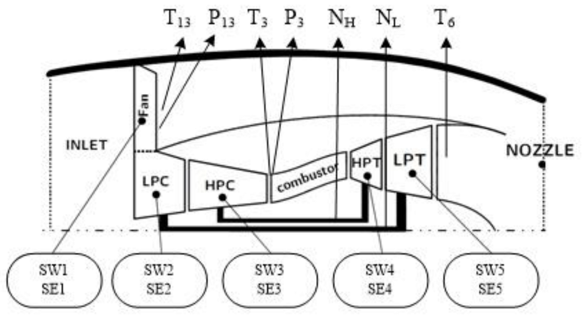
All simulation data are obtained using TurboFan Engine Simulator. By inputting a specific working condition, the simulation software can calculate the performance parameters under the condition.

First a fleet of engines is simulated. The system’s components will experience degradation due to wear and tear resulting from usage. It is most often a slow phenomenon, which is detected relative to past performance on the same engine. It is very difficult to detect an efficiency drop in absolute value, because each unit of the fleet has slightly different initial wear at the engine sub-component due to manufacturing and assembly tolerances, which leads to differences in the health parameters of each engine component in the fleet, such as efficiency and flow.

For the above reasons, each engine in the startup fleet can be distinguished based on the difference in the initial health parameters. Assuming that the deviation between the health parameters of a specific engine unit and the baseline value conform to a triangular distribution, the maximum and minimum deviation values of the parameters of each component are shown in

Table 4. Health Parameter Deviation.

Health Parameter	Minimum Deviation	Maximum Deviation
Fan flow correction factor SW1 (%)	−1	1
Fan efficiency correction factor SE1 (%)	−0.3	0.1
LPC flow correction factor SW2 (%)	−1	1
LPC efficiency correction factor SE2 (%)	−1	0.5
HPC flow correction factor SW3 (%)	−1	1
HPC efficiency correction factor SE3 (%)	−0.6	0.6
HPT flow correction factor SW4 (%)	−1.5	1.5
HPT efficiency correction factor SE4 (%)	−0.35	0.15
LPT flow correction factor SW5 (%)	−0.5	0.5
LPT efficiency correction factor SE5 (%)	−0.5	0.5

.

Based on the triangular distribution of the parameters, this paper adopts the Monte Carlo idea to randomly select values, and generates 100 sets of unit body health parameter deviation values, and uses this to distinguish each specific engine. Figure 5 shows the triangular distribution of Fan efficiency deviation.

After obtaining the fleet data, the next step is to simulate different take-off conditions for each individual engine. Each set of different takeoff conditions simulation represents a specific flight. The simulation method is the same as the fleet data. Assuming that the parameters of the take-off condition also conform to the triangular distribution, the maximum and minimum deviation values are shown in

Table 5. Condition Parameter Deviation.

Condition Parameters	Minimum Deviation	Maximum Deviation
Altitude (m)	−500	500
Mach number	0.24	0.26
Standard atmospheric temperature difference (C)	−20	20
Fuel flow (kg/s)	0.83	0.97

.

Each engine randomly generates 1000 sets of condition parameter values for flights simulation. After the simulation calculation is completed, the performance data of 100 engines is obtained, and 1000 flights are simulated for each engine. The gas path parameters calculated with the aid of the performance model do not contain noise, but in practice the sensor will inevitably introduce measurement noise. Therefore, a certain amount of Gaussian noise is added to the gas path parameters to simulate actual measurement noise.

4.2. Data Preprocessing and Fault Injection

The baseline model of engine can reflect the basic functional relationships of engine performance parameters in a healthy state. When the engine is in a healthy state, the performance parameter deviation value obtained by subtracting the baseline value from the actual measurement value should theoretically fluctuate around 0. The abnormal detection of the engine performance parameter can be realized by analyzing the deviation value sequence.

The performance measurement deltas ($\Delta Y$) of each parameter needs to be calculated to facilitate the detection of the algorithm. The formula is as follows:

$$\Delta Y=Y-Y_0$$

(1)

where Y represents the value of the parameter, and Y₀ the nominal value at a typical taking-off condition when the engine is at a clean and new condition. (That is, using the Random Forest algorithm for parameter regression).

The health parameter deviation is calculated as follows:

$$\Delta f=(f-f_0)\cdot 100\%$$

(2)

where f₀ = 1 meaning the engine is at a clean and new condition. The interrelation among the health parameters deviations and the measurements deltas is expressed through a multi variable regression model, which is obtained by linearizing of the engine performance model at a typical taking-off operating point.

In this paper, two kinds of baseline values Y₀ are calculated. One is to randomly select 400 sets of data from all health status data of the fleet to calculate a baseline value. The other is based on the first 400 health data of each engine, a total of 20 engines’ personalized baseline values was established separately.

Component faults are simulated by deviating of the corresponding health parameters from their nominal values, i.e., the flow and efficiency deviations of each module. To demonstrate the proposed information fusion mechanism, a typical set of fault scenarios has been examined, which covers different possible faults in all individual components (given in

Table 6. Failure modes.

Failure Modes	Changes in Health Parameters
Failure mode A	Fan flow rate drops by 1%, efficiency drops by 1.5%
Failure mode B	HPC flow rate drops by 1%, efficiency drops by 0.7%
Failure mode C	HPT flow rate drops by 1%, efficiency drops by 1%
Failure mode D	LPT flow rate drops by 1%, efficiency drops by 0.5%
Failure mode E	HPC efficiency decreased by 1.5%
Failure mode F	HPT efficiency decreased by 1.5%

).

For each fault case, a series of n = 400 measurement sets from the taking-off operating point has been recorded for following, including 20 fleet samples and 20 single engine samples. They were randomly selected from the fleet data without putting it back. The first 360 sets are health status data, and the last 40 sets are abnormal conditions (Inject according to the failure mode of Table 4).

4.3. Results Analysis and Comparison

In the detection, four binary classifiers, IForest, XGBOD, MCD, OCSVM (one class support vector machine), are chosen as detection algorithms. The algorithms will output two indicators to measure classification accuracy: AUC and Precision. AUC is the area under the ROC curve, its value is equivalent to the probability that a randomly chosen positive example is ranked higher than a randomly chosen negative example. As for precision, it is the probability of how many real positive examples are in the sample predicted to be positive.

This article compares the test results from the following three aspects:

• Comparison of anomaly detection effects between the fleet baseline model and a single personalized baseline model:

The deviation values obtained from the two baseline models are input into the isolation forest, MCD, XGBOD, OCSVM algorithm. The AUC value and accuracy rate of the abnormal detection of six abnormal modes is calculated by the algorithm model. Since each algorithm has been tested many times, the calculation result is the average of multiple tests. After detection, the comparison of AUC and precision is shown in the figure below.

It can be seen from Figure 6 and Figure 7 that only three faults (i.e., fault C, D and E) have relatively high detection accuracy. The remaining fault cases are misdiagnosed. Among the four anomaly detection algorithms, XGBOD is an ensemble learning algorithm, so the overall effect is the best. The overall anomaly detection effect of MCD and IForest is not much different. In abnormal modes A and F, IForest is better than MCD. In abnormal mode B, MCD is better than IForest. OCSVM has the worst anomaly detection effect overall.

2.

The influence of engine performance parameters on anomaly detection effect:

In the above, the deviation values of the nine performance parameters are all detected for abnormality. In the actual situation, the data collected by the sensor does not include the HPC inlet pressure and inlet temperature. Therefore, this section will compare the anomaly detection effects of the nine parameters and the seven parameters.

Table 7. Detection Results (AUC).

Failure Modes	IForest		XGBOD		MCD		OCSVM
	Nine PARAM	Seven PARAM	Nine PARAM	Seven PARAM	Nine PARAM	Seven PARAM	Nine PARAM	Seven PARAM
A	0.89	0.81	0.98	0.92	0.88	0.89	0.83	0.83
B	0.90	0.85	0.99	0.98	0.96	0.92	0.76	0.75
C	0.99	0.99	1.0	1.0	0.99	0.99	0.99	0.99
D	0.98	0.99	0.99	0.99	0.99	0.99	0.98	0.98
E	0.99	0.99	1.0	1.0	1.0	1.0	1.0	1.0
F	0.94	0.95	0.99	0.99	0.91	0.91	0.93	0.94

and

Table 8. Detection Results (precision).

Failure Modes	IForest		XGBOD		MCD		OCSVM
	Nine PARAM	Seven PARAM	Nine PARAM	Seven PARAM	Nine PARAM	Seven PARAM	Nine PARAM	Seven PARAM
A	0.49	0.36	0.78	0.71	0.51	0.53	0.41	0.41
B	0.48	0.43	0.90	0.79	0.74	0.57	0.20	0.19
C	0.94	0.90	0.99	0.99	0.93	0.96	0.98	0.98
D	0.85	0.83	0.98	0.97	0.92	0.94	0.86	0.86
E	0.97	0.98	1.0	1.0	1.0	1.0	1.0	1.0
F	0.66	0.72	0.92	0.91	0.59	0.62	0.73	0.73

show the results.

The failure modes not accurately identified were failure mode A and B. For the failure mode B, the HPC fault with a simultaneous reduction in efficiency and flow capacity, which may affect LPC component, resulting in an evident LPC efficiency decrease. Due to the limited on-board performance measurement set, the measurements between the LPC and HPC are insufficient to characterize all fault information, for which they share a similar measurement observation pattern due to the failure.

3.

The influence of different levels of noise on the detection effect:

Besides the on-board sensor measurements limitation, the measurement noise can also introduce uncertainty into the health parameters estimation. Especially when the fault magnitude is relatively smaller, the failure signature maybe masked in the measurement noise, causing wrong diagnostics conclusions. Two types of noise are used to process the data here. The amount of noise is shown in

Table 9. Noise Setting.

Gas Path Performance Parameter	Noise A	Noise B
Outlet pressure of the fan P13 (bar)	0.25%	0.5%
Outlet temperature of the fan T13 (C)	0.4%	0.8%
Inlet pressure of HPC P2 (bar)	0.25%	0.5%
Inlet temperature of HPC T2 (C)	0.4%	0.8%
Outlet temperature of the HPC T3 (C)	0.25%	0.5%
Outlet pressure of the HPC P3 (bar)	0.4%	0.8%
Exhaust gas temperature T6 (C)	0.4%	0.8%
Low pressure rotor speed NL (rpm)	0.05%	0.1%
High pressure rotor speed NH (rpm)	0.05%	0.1%

.

The test analysis for the above test results is given here. First, in the detection of different baseline model, the failure modes B, C, D, E and F show better effect with single engine baseline model. However, in the detection of failure mode A, the detection effect of the fleet baseline model is more accurate, which means that the failure mode A is less affected by the engine’s performance difference. The fan is the most exposed air path component of the engine. Compared to changes in internal flow and efficiency of components, changes in the external environment are more likely to affect the efficiency of the fan.

Second, most algorithms obtain better detection results when the input performance parameters are nine. However, the MCD algorithm performs even better when the input parameters are seven, which may be related to the internal calculation of the Mahalanobis distance. When the dimensionality of the data point increases, the calculated Mahalanobis distance will also increase. If the fault information can be reflected by only a few parameters, adding more parameter dimension may cover up the fault information which needs to be expressed by the value of distance, and it may lead to the misjudgment of the algorithm.

Third, the detection results of noise case are given in

Table 10. Detection Result of Different Noise.

Failure Modes	IForest		XGBOD		MCD		OCSVM
	Noise A	Noise B	Noise A	Noise B	Noise A	Noise B	Noise A	Noise B
A	0.49	0.42	0.78	0.72	0.51	0.56	0.41	0.31
B	0.48	0.48	0.89	0.73	0.74	0.59	0.20	0.37
C	0.94	0.73	0.99	0.99	0.93	0.71	0.98	0.92
D	0.85	0.75	0.98	0.97	0.92	0.83	0.86	0.85
E	0.97	0.94	1.0	1.0	1.0	0.99	1.0	1.00
F	0.65	0.49	0.92	0.80	0.59	0.33	0.73	0.66

. Indicator “Precision” is more obviously affected by noise, so it is selected as the observation target.

It can be observed that the detection ability of all algorithms decreases after the noise is doubled. Among them, the detection accuracy of failure modes C, D and F are significantly reduced, which are all turbine failure. This shows the flow and efficiency deviations of turbine component have less impact on the engine, which can be easily masked in the noise.

Based on the above results, the XGBOD algorithm has the highest detection accuracy. It makes good use of its advantages as an integrated algorithm, and performs well in the case of reduced parameters or increased noise. In contrast, the detection accuracy of IForest and OCSVM algorithms is not in a good level. Due to the lack of training data, the IForest failed to play its advantage in the detection of massive data. As for OCSVM, it is mainly good at single classification [28], and it does not perform well on two classification problems.

In terms of failure modes, failure mode E has the highest detection accuracy. This shows that the reduced efficiency of the high-pressure compressor will seriously affect the performance of the whole engine. On the other hand, the detection rate of each algorithm for failure mode A is relatively low. The reason may be that the selected parameters cannot well represent the characteristics of the failure, or the failure itself has a small impact on engine’s performance.

5. Conclusions

This paper presents a detailed review of an experimental data mining algorithm library for engine condition monitoring, which comprises different types of algorithms (baseline construction, anomaly detection, trend prediction). The algorithm library is validated on engine simulation data, which shows great effectiveness on detecting different types of failure.

The innovations of the algorithm library are listed below:

• This algorithm library is specifically established for engine condition monitoring;
• The simulation data set used in this article can be made public for verification by other anomaly detection algorithm developers;
• Compare the performance differences in anomaly detection algorithms in each condition to provide reference for actual engineering applications.

In the case study part of the paper, the performance data simulation of the engine fleet’s health status and abnormal conditions is carried out. The baseline models of the fleet and a single engine are established respectively, and the deviation value sequences obtained from different baseline models are compared for anomaly detection. This paper tested four anomaly detection algorithms: Isolated Forest, XGBOD, MCD, OCSVM. The conclusions are as follows:

• Different abnormal modes have different effects on engine performance parameters, leading to different detection results. The overall HPC and HPT abnormal detection results are the best;
• In the comparison of the four algorithms, the XGBOD anomaly detection based on the integrated idea is the most accurate and can detect most outliers;
• In terms of the deviation value sequences obtained by different baseline models, the individualized model is slightly better than the fleet model based on the fleet data in anomaly detection;
• The reduction in status monitoring parameters and increased noise will reduce the accuracy of detection.

The successful application of these algorithms proves the reliability and efficiency of the algorithm library. To further improve the performance of the algorithm library, different operating conditions still need to be investigated. Therefore, a potential future research direction is a validation on actual failure data, as well as the installation of new algorithms.