
Data Driven Modal Decomposition of the Wake behind an NREL-5MW Wind Turbine †


 and
and 
Abstract
:1. Introduction
2. Methodology
2.1. Proper Orthogonal Decomposition
2.2. Sparsity-Promoting Dynamic Mode Decomposition
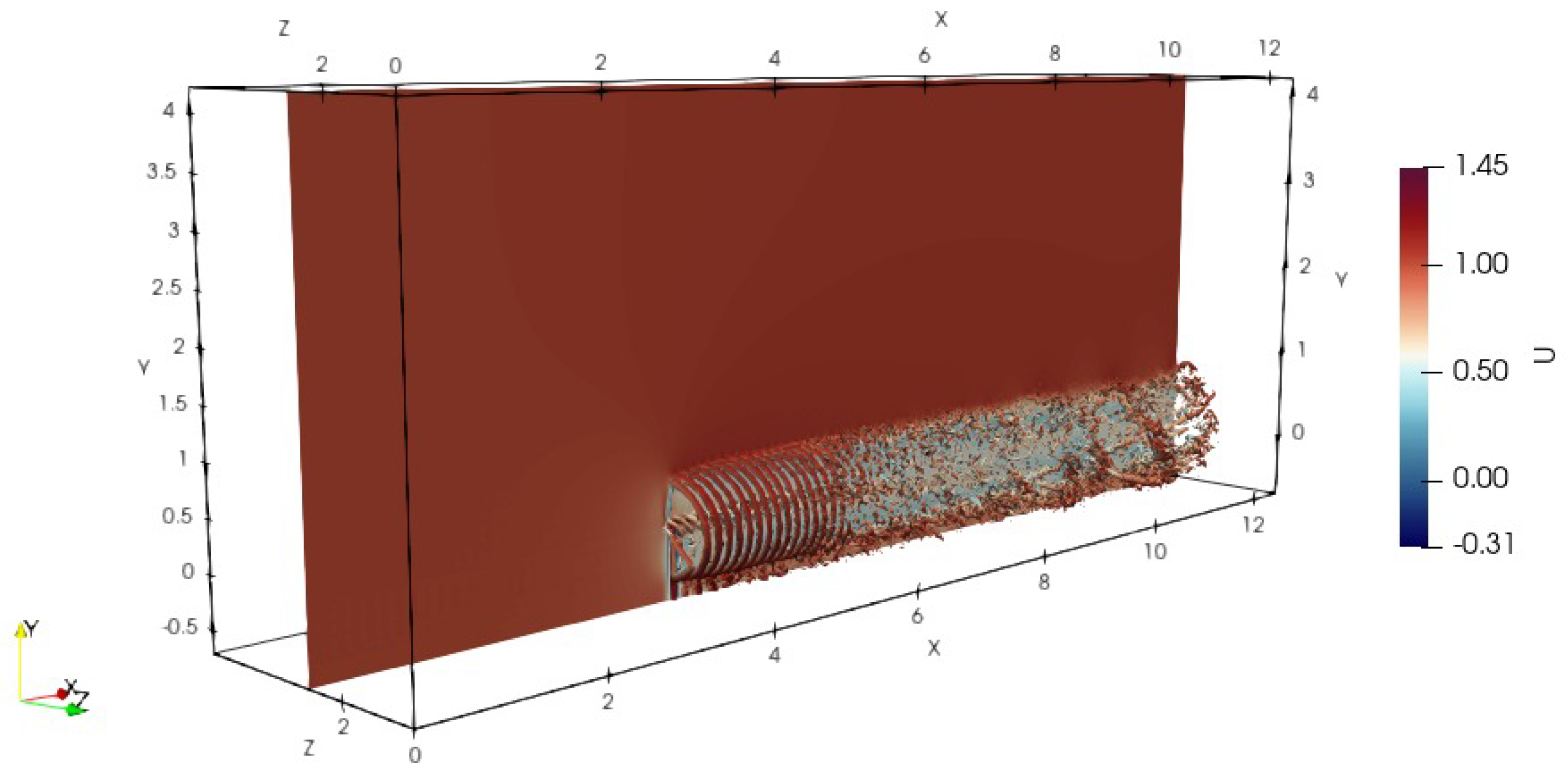
3. Simulation Setup
4. Modal Decomposition of the Wake
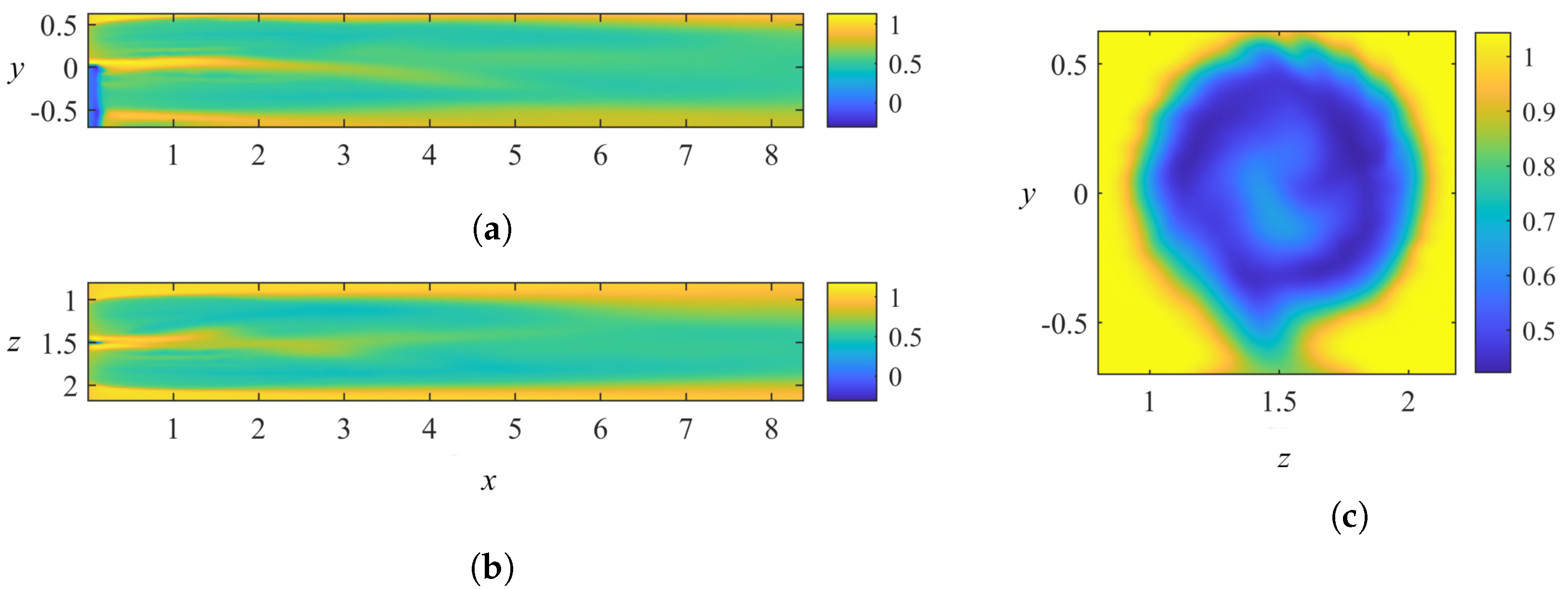
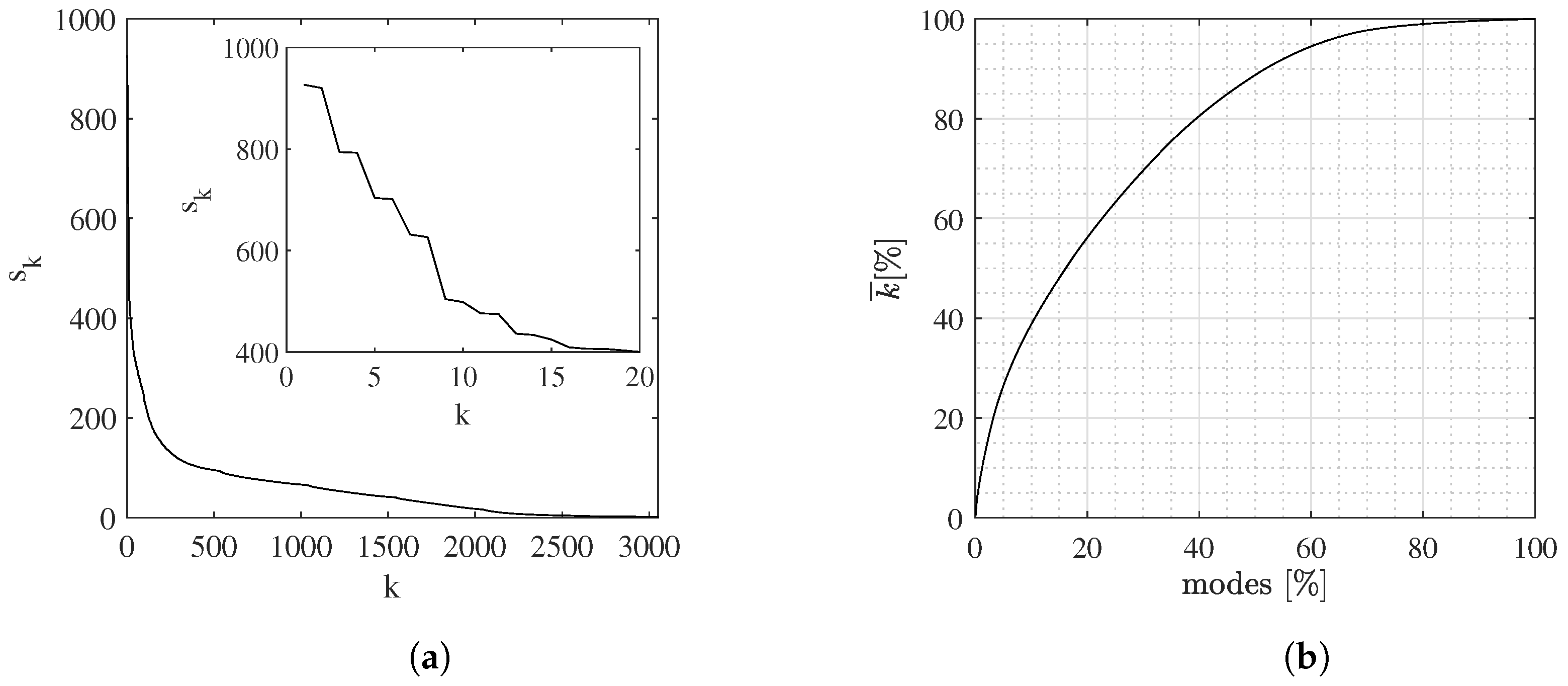
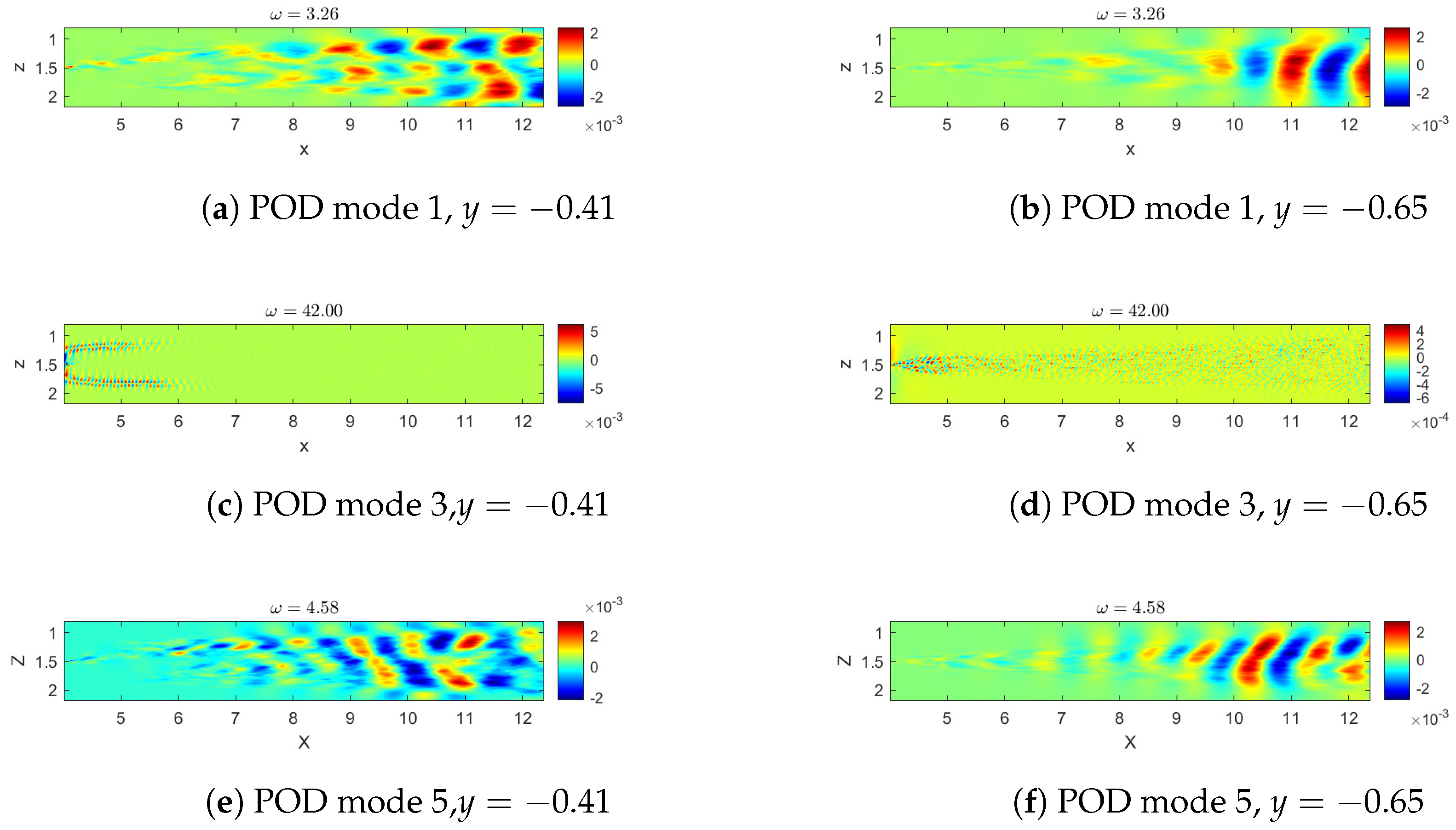
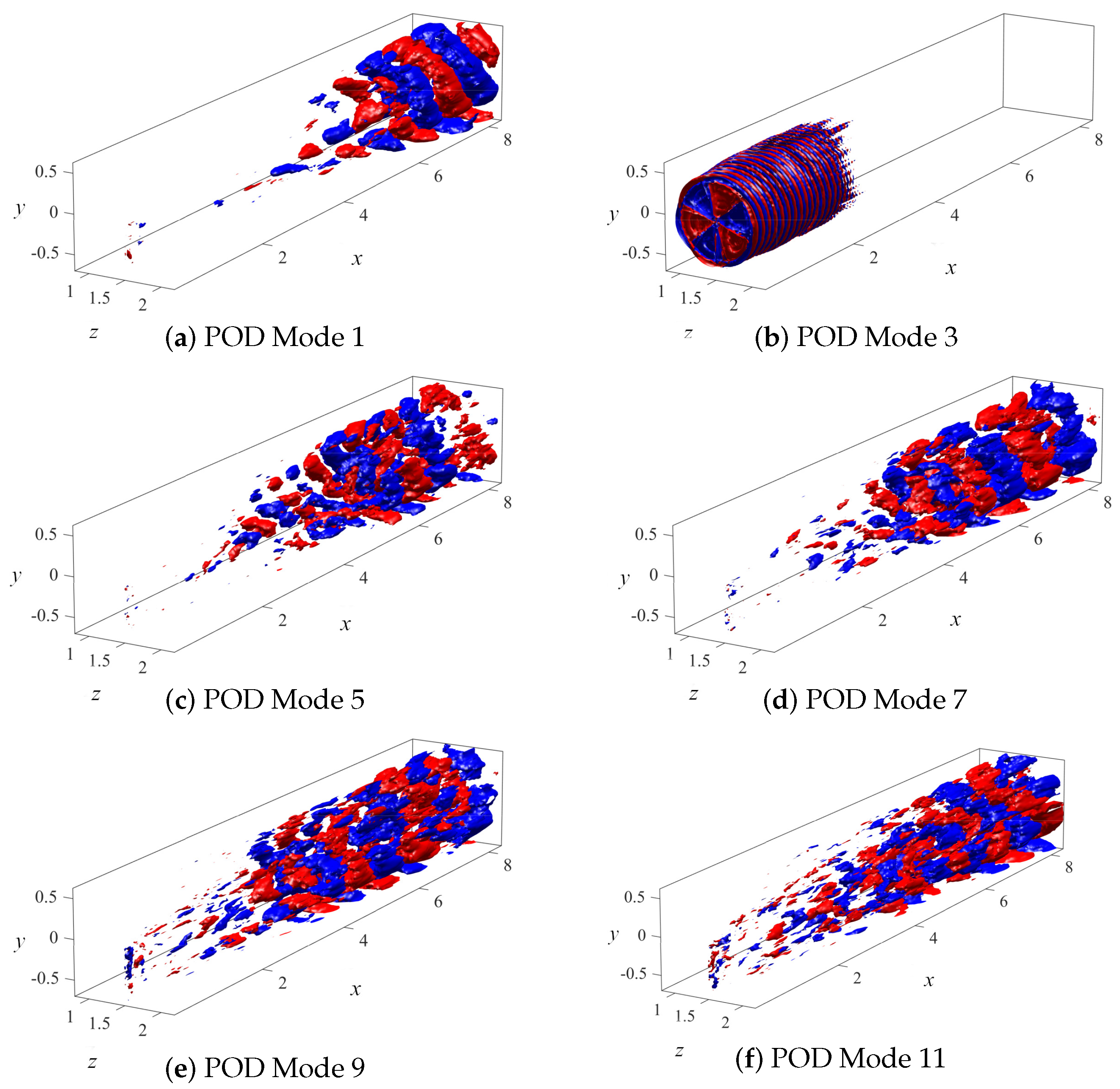
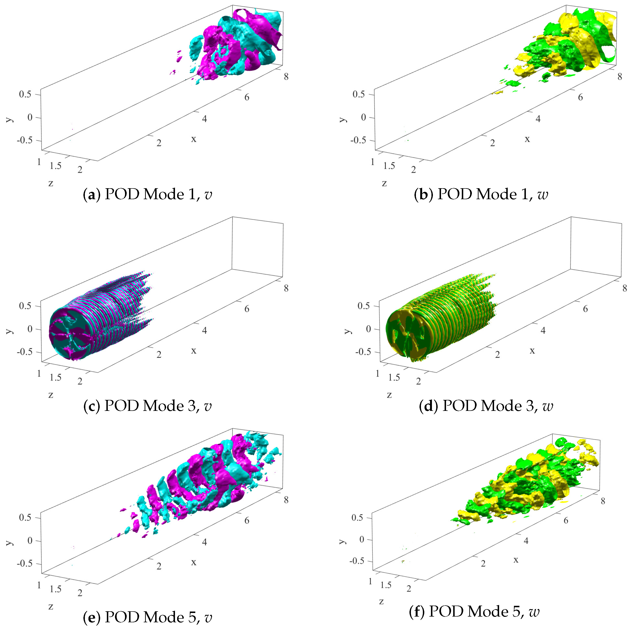
4.1. POD Results
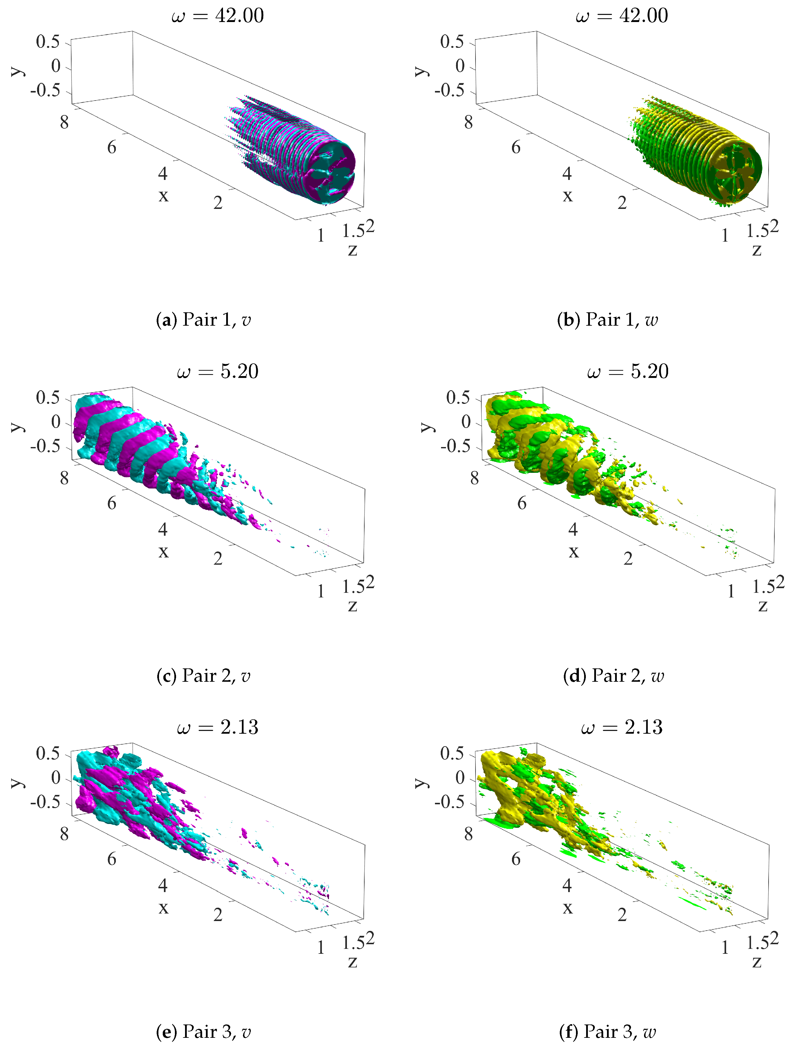
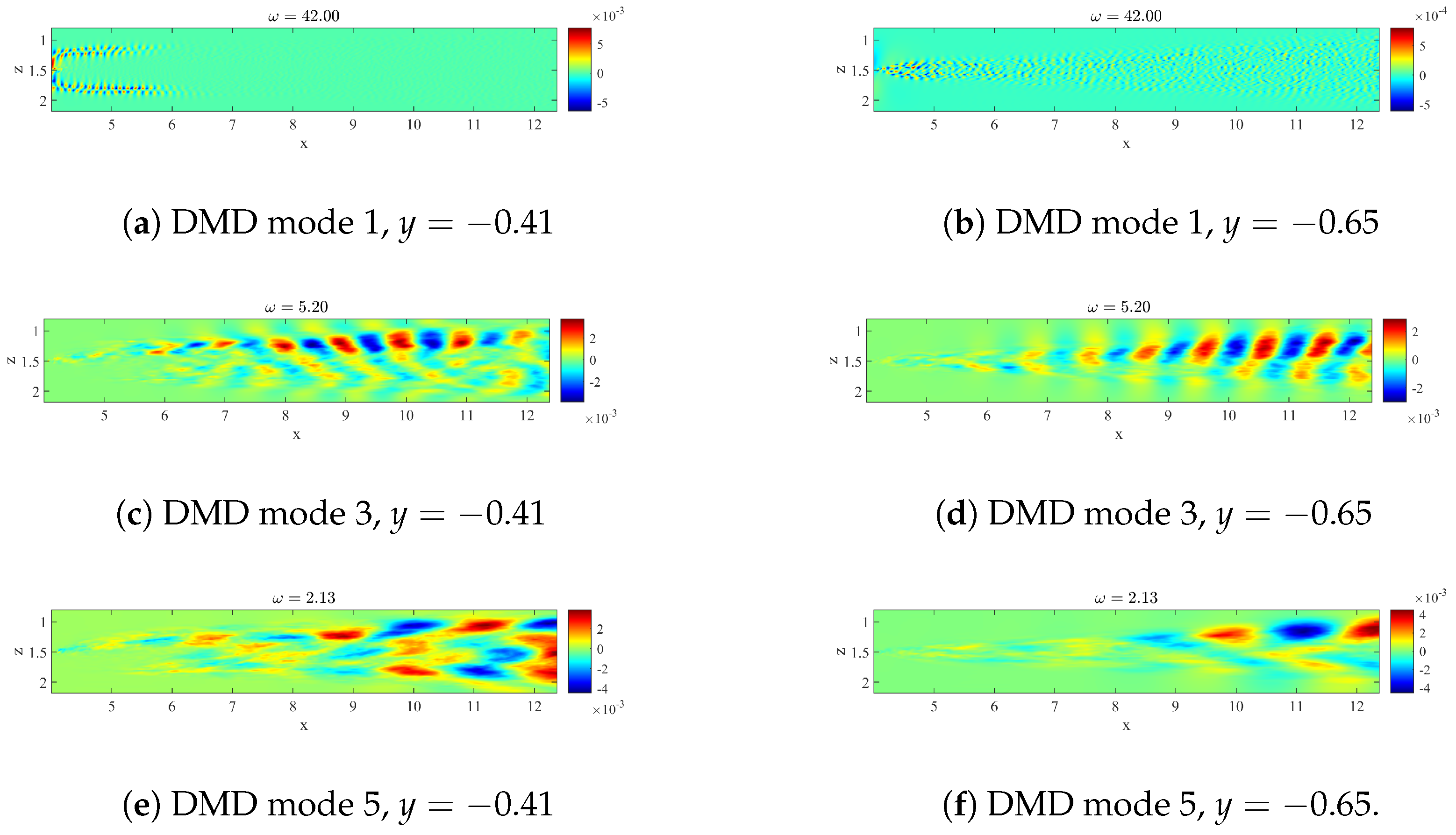
4.2. SP-DMD Results
5. Discussion
6. Conclusions
Author Contributions
Funding
Institutional Review Board Statement
Informed Consent Statement
Data Availability Statement
Conflicts of Interest
References
- Andersen, S.J.; Sørensen, J.N.; Mikkelsen, R. Simulation of the inherent turbulence and wake interaction inside an infinitely long row of wind turbines. J. Turbul. 2013, 14, 1–24. [Google Scholar] [CrossRef]
- Bastine, D.; Witha, B.; Wächter, M.; Peinke, J. Towards a simplified dynamicwake model using pod analysis. Energies 2015, 8, 895–920. [Google Scholar] [CrossRef] [Green Version]
- VerHulst, C.; Meneveau, C. Large eddy simulation study of the kinetic energy entrainment by energetic turbulent flow structures in large wind farms. Phys. Fluids 2014, 26, 025113. [Google Scholar] [CrossRef]
- Hamilton, N.; Tutkun, M.; Cal, R.B. Wind turbine boundary layer arrays for Cartesian and staggered configurations: Part II, low-dimensional representations via the proper orthogonal decomposition. Wind Energy 2015, 18, 297–315. [Google Scholar] [CrossRef]
- Hamilton, N.; Tutkun, M.; Cal, R.B. Anisotropic character of low-order turbulent flow descriptions through the proper orthogonal decomposition. Phys. Rev. Fluids 2017, 2, 014601. [Google Scholar] [CrossRef]
- Hamilton, N.; Viggiano, B.; Calaf, M.; Tutkun, M.; Cal, R.B. A generalized framework for reduced-order modeling of a wind turbine wake. Wind Energy 2018, 21, 373–390. [Google Scholar] [CrossRef]
- Fortes-Plaza, A.; Campagnolo, F.; Wang, J.; Wang, C.; Bottasso, C. A POD reduced-order model for wake steering control. J. Phys. Conf. Ser. 2018, 1037, 032014. [Google Scholar] [CrossRef]
- De Cillis, G.; Cherubini, S.; Semeraro, O.; Leonardi, S.; De Palma, P. POD-based analysis of a wind turbine wake under the influence of tower and nacelle. Wind Energy 2021, 24, 609–633. [Google Scholar] [CrossRef]
- Ilak, M.; Rowley, C.W. Modeling of transitional channel flow using balanced proper orthogonal decomposition. Phys. Fluids 2008, 20, 034103. [Google Scholar] [CrossRef] [Green Version]
- Schmid, P.J. Dynamic mode decomposition of numerical and experimental data. J. Fluid Mech. 2010, 656, 5–28. [Google Scholar] [CrossRef] [Green Version]
- Iungo, G.V.; Santoni-Ortiz, C.; Abkar, M.; Porté-Agel, F.; Rotea, M.A.; Leonardi, S. Data-driven reduced order model for prediction of wind turbine wakes. J. Phys. Conf. Ser. 2015, 625, 012009. [Google Scholar] [CrossRef]
- Le Clainche, S.; Lorente, L.S.; Vega, J.M. Wind predictions upstream wind turbines from a LiDAR database. Energies 2018, 11, 543. [Google Scholar] [CrossRef] [Green Version]
- Chen, K.K.; Tu, J.H.; Rowley, C.W. Variants of dynamic mode decomposition: Boundary condition, Koopman, and Fourier analyses. J. Nonlinear Sci. 2012, 22, 887–915. [Google Scholar] [CrossRef]
- Jovanović, M.R.; Schmid, P.J.; Nichols, J.W. Sparsity-promoting dynamic mode decomposition. Phys. Fluids 2014, 26, 024103. [Google Scholar] [CrossRef]
- Semeraro, O.; Bellani, G.; Lundell, F. Analysis of time-resolved PIV measurements of a confined turbulent jet using POD and Koopman modes. Exp. Fluids 2012, 53, 1203–1220. [Google Scholar] [CrossRef]
- Frederich, O.; Luchtenburg, D.M. Modal analysis of complex turbulent flow. In Seventh International Symposium on Turbulence and Shear Flow Phenomena; Begell House Digital Library: Danbury, CT, USA, 2011. [Google Scholar]
- Muld, T.W.; Efraimsson, G.; Henningson, D.S. Flow structures around a high-speed train extracted using Proper Orthogonal Decomposition and Dynamic Mode Decomposition. Comput. Fluids 2012, 57, 87–97. [Google Scholar] [CrossRef]
- Mendez, M.; Balabane, M.; Buchlin, J.M. Multi-scale proper orthogonal decomposition of complex fluid flows. J. Fluid Mech. 2019, 870, 988–1036. [Google Scholar] [CrossRef] [Green Version]
- Medici, D. Experimental Studies of Wind Turbine Wakes: Power Optimisation and Meandering. Ph.D. Thesis, Kungliga Tekniska Hogskolan (KTH), Stockholm, Sweden, 2005. [Google Scholar]
- Pope, S.; Pope, S.; Eccles, P.; Press, C.U. Turbulent Flows; Cambridge University Press: Cambridge, UK, 2000. [Google Scholar]
- Orlandi, P. Fluid Flow Phenomena: A Numerical Toolkit; Volume 55, Fluid Mechanics and Its Applications; Springer: Dordrecht, The Netherlands, 2000. [Google Scholar] [CrossRef]
- Sørensen, J.N.; Shen, W.Z. Computation of wind turbine wakes using combined Navier-Stokes/actuator-line Methodology. In Proceedings of the 1999 European Wind Energy Conference and Exhibition, Nice, France, 1–5 March 1999; pp. 156–159. [Google Scholar]
- Orlandi, P.; Leonardi, S. DNS of turbulent channel flows with two-and three-dimensional roughness. J. Turbul. 2006, 7, N73. [Google Scholar] [CrossRef]
- Orlanski, I. A simple boundary condition for unbounded hyperbolic flows. J. Comput. Phys. 1976, 21, 251–269. [Google Scholar] [CrossRef]


| -POD | -DMD | (std. DMD) | (SP-DMD) | |
|---|---|---|---|---|
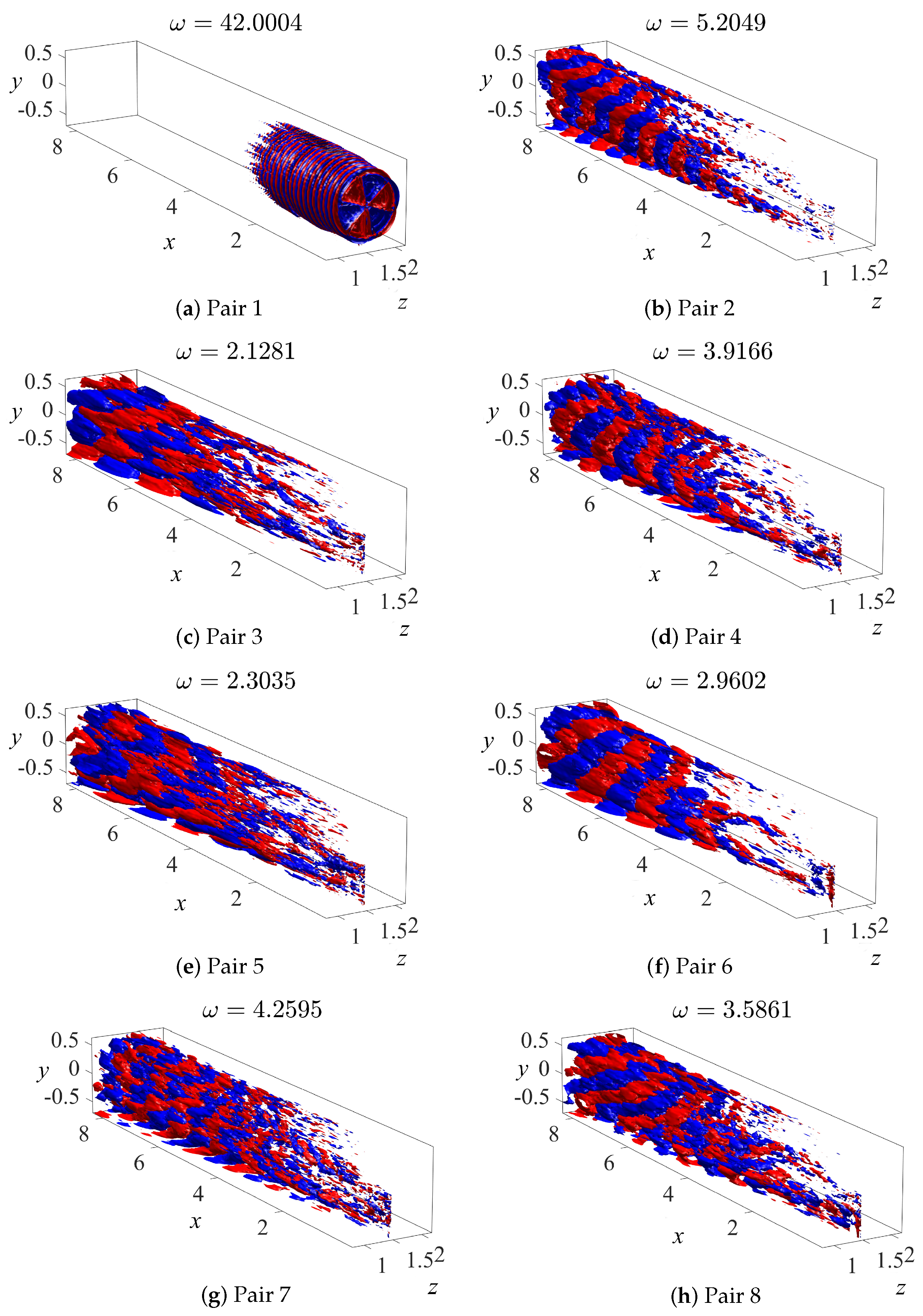
| Pair 1 | 3.26 | 42.0 | 14.34 | 14.86 |
| Pair 2 | 42.0 | 5.20 | 11.39 | 9.55 |
| Pair 3 | 4.58 | 2.13 | 8.54 | 8.53 |
| Pair 4 | 2.23 | 3.92 | 9.26 | 7.89 |
| Pair 5 | 2.44 | 2.30 | 7.50 | 7.80 |
| Pair 6 | 3.76 | 2.96 | 8.26 | 7.48 |
| Pair 7 | 2.64 | 4.25 | 6.39 | 6.02 |
| Pair 8 | 1.13 | 3.58 | 4.22 | 4.06 |
Publisher’s Note: MDPI stays neutral with regard to jurisdictional claims in published maps and institutional affiliations. |
© 2021 by the authors. Licensee MDPI, Basel, Switzerland. This article is an open access article distributed under the terms and conditions of the Creative Commons Attribution (CC BY-NC-ND) license (https://creativecommons.org/licenses/by-nc-nd/4.0/).
Share and Cite
Cherubini, S.; De Cillis, G.; Semeraro, O.; Leonardi, S.; De Palma, P. Data Driven Modal Decomposition of the Wake behind an NREL-5MW Wind Turbine. Int. J. Turbomach. Propuls. Power 2021, 6, 44. https://doi.org/10.3390/ijtpp6040044
Cherubini S, De Cillis G, Semeraro O, Leonardi S, De Palma P. Data Driven Modal Decomposition of the Wake behind an NREL-5MW Wind Turbine. International Journal of Turbomachinery, Propulsion and Power. 2021; 6(4):44. https://doi.org/10.3390/ijtpp6040044
Chicago/Turabian StyleCherubini, Stefania, Giovanni De Cillis, Onofrio Semeraro, Stefano Leonardi, and Pietro De Palma. 2021. "Data Driven Modal Decomposition of the Wake behind an NREL-5MW Wind Turbine" International Journal of Turbomachinery, Propulsion and Power 6, no. 4: 44. https://doi.org/10.3390/ijtpp6040044
APA StyleCherubini, S., De Cillis, G., Semeraro, O., Leonardi, S., & De Palma, P. (2021). Data Driven Modal Decomposition of the Wake behind an NREL-5MW Wind Turbine. International Journal of Turbomachinery, Propulsion and Power, 6(4), 44. https://doi.org/10.3390/ijtpp6040044