Article

Analysis of a Linear Model for Non-Synchronous Vibrations Near Stall †

by
Christoph Brandstetter
1,*,‡ and
Sina Stapelfeldt
2,‡
1
Ecole Centrale de Lyon, Universite de Lyon, CNRS, Universite Claude Bernard Lyon 1, INSA Lyon, LMFA, UMR 5509, F-69134 Ecully, France
2
Department of Mechanical Engineering, Imperial College London, London SW7 2AZ, UK
*
Author to whom correspondence should be addressed.
This paper is an extended version of our paper published in the Proceedings of the 14th European Turbomachinery Conference, Gdansk, Poland, 12–16 April 2021.
These authors contributed equally to this work.
Int. J. Turbomach. Propuls. Power 2021, 6(3), 26; https://doi.org/10.3390/ijtpp6030026
Submission received: 30 June 2021 / Revised: 6 July 2021 / Accepted: 6 July 2021 / Published: 9 July 2021

Abstract

:
Non-synchronous vibrations arising near the stall boundary of compressors are a recurring and potentially safety-critical problem in modern aero-engines. Recent numerical and experimental investigations have shown that these vibrations are caused by the lock-in of circumferentially convected aerodynamic disturbances and structural vibration modes, and that it is possible to predict unstable vibration modes using coupled linear models. This paper aims to further investigate non-synchronous vibrations by casting a reduced model for NSV in the frequency domain and analysing stability for a range of parameters. It is shown how, and why, under certain conditions linear models are able to capture a phenomenon, which has traditionally been associated with aerodynamic non-linearities. The formulation clearly highlights the differences between convective non-synchronous vibrations and flutter and identifies the modifications necessary to make quantitative predictions.

1. Introduction

The drive towards reduced engine weight and fuel burn has pushed compressors towards lighter designs with increased stage loading, leading to a rise of non-synchronous vibrations (NSV) near the stall boundary. The term ‘non-synchronous vibration’ generally encompasses any vibration at frequencies which are not integer multiples of the shaft frequency, i.e., frequencies not induced by engine-order excitations. This includes buffeting, rotating stall and self-excited vibrations (flutter). In recent literature, however, the term NSV has often been used to describe a subset of non-synchronous vibrations, where circumferentially propagating aerodynamic disturbances lock in with the rotor’s natural vibration modes, and this terminology is adapted in this Introduction.
Without extensive instrumentation or detailed numerical analysis, it is often impossible to distinguish between different types of non-integral vibrations. Throughout the history of turbomachines, controversies around vibrations near the stall boundary have been recognised [1]. It has been questioned whether vibrations caused by stall flutter [2], rotating stall [3], unstable/stable stall [4] and ‘NSV’ [5] have distinct root causes or are simply different terms for one phenomenon. This paper aims to demonstrate the differences between NSV and flutter by explaining the physical mechanisms responsible for NSV and comparing a reduced order model for its prediction against flutter models.
To outline the similarities between the two phenomena, we first review them. Flutter is a self-excited aeroelastic instability, where aerodynamic forces amplify the vibration. It often, but not exclusively, occurs at the stall boundary and its defining criteria are:
  • The aeroelastic system is linearly unstable.
  • The unsteady aerodynamic forces are generated by the blade vibration, i.e., the instability requires the participation of the structure.
Although the aerodynamics involved in flutter are often non-linear, linear theory is used to discriminate between stability and instability. For quantitative predictions of blade amplitudes and stresses during flutter, non-linearities must be taken into account. For a more detailed discussion of flutter the reader is referred to, for example, the work of Sisto [1], Carter and Kilpatrick [6], Corral [7] or Duquesne et al. [8].
Compared to flutter, NSV is less well defined and therefore warrants a summary of recent literature. One frequently cited study on NSV was published by Baumgartner et al. [9] and discusses the excitation of structural vibration modes by so-called ‘rotating instabilities’, aerodynamic disturbances which propagate around the circumference. The paper has received a lot of attention, but it delivers few physical explanations regarding the nature of these disturbances or the mechanisms by which fluid and structure couple. (In the authors’ opinion, the interpretation in this paper is misleading, and an interpretation of the measured data which is consistent with the latest understanding of NSV is possible [10]). Kielb et al. [5] provided a physical explanation of NSV in the front stages of a compressor rig. The vibrations resembled flutter but typical flutter parameters, such as reduced frequency, incidence angle and Mach number, were uncharacteristically high, and the frequency of vibration measured differed from the in-vacuo structural frequency. Subsequent studies indicated that the source of vibration was an aerodynamic instability which locked in with a rotor vibration mode. The conceptual understanding of this study has underpinned many subsequent studies, and, in the majority of these, vibrations occurred close to stall and have been associated with stall precursors (but not with rotating stall). Vo et al. [11] and later Vo [12], for example, reported non-synchronous vibrations after stall criteria, such as leading edge spillage and trailing edge back-flow, were met and short length-scale pre-stall disturbances, known as spikes, developed. Brandstetter et al. [13] used experiments on a transonic research compressor to show how a circumferentially propagating vortical disturbance locked in with rotor vibrations in the first torsional eigenmode. The vortical disturbance which existed before onset of vibration also resembled stall precursors previously identified as ‘radial vortices’ [14,15,16]. A subsequent numerical study by Stapelfeldt and Brandstetter [17] investigated the influence of various parameters on the lock-in phenomenon and made it possible to qualitatively and quantitatively relate the circumferentially convected vortical disturbance to the aerodynamic forcing and resulting blade deflections. In this work, we propose the term ‘convective NSV’ to differentiate this particular type of non-synchronous vibration from others, such as flutter or vibrations driven by acoustic resonances or vortex shedding. Using the knowledge gathered during the last 20 years, the characteristics of convective NSV can be summarised as follows:
  • It occurs near the stall boundary but before rotating stall cells form.
  • Prior to convective NSV, frequency spectra of unsteady pressure contain broadband frequencies, which result from multi-wave number disturbances propagating at approximately 50% of the rotor speed in the direction opposing rotation (in the rotor frame of reference).
  • At the onset of vibration, the aerodynamic disturbance locks in with the structural vibration and the broadband spectrum changes to a coherent aerodynamic disturbance with a distinct frequency peak.
Two important criteria must be fulfilled for it to occur:
  • The mean aerodynamics must promote the circumferential convection of vorticity, i.e., the blade must react to small changes in incidence by shedding vorticity, while the passage must be blocked close to the casing to allow the circumferential transport.
  • The blade vibration must be able to modulate the propagation velocity of the aerodynamic disturbance to create a coherent disturbance in resonance with the vibration pattern.
Following the description of the phenomenon in [17], we present a semi-analytical model based on forced single-degree of freedom oscillators to predict unstable vibration modes. The aerodynamic forcing term in this model is linearly dependent on the blade-deflection amplitude, although non-linearities are observed for high blade vibration amplitudes. At first sight, the phenomenon could be mistaken as flutter, satisfying both of the characteristic criteria listed above. This and the similarities in experimental signatures of flutter and NSV renewed doubt on the distinction between the two. The aim of the current paper is to further analyse the reduced order model in order to clearly illustrate why flutter and convective NSV are two different phenomena.

2. Review of NSV Model

The model presented by Stapelfeldt and Brandstetter [
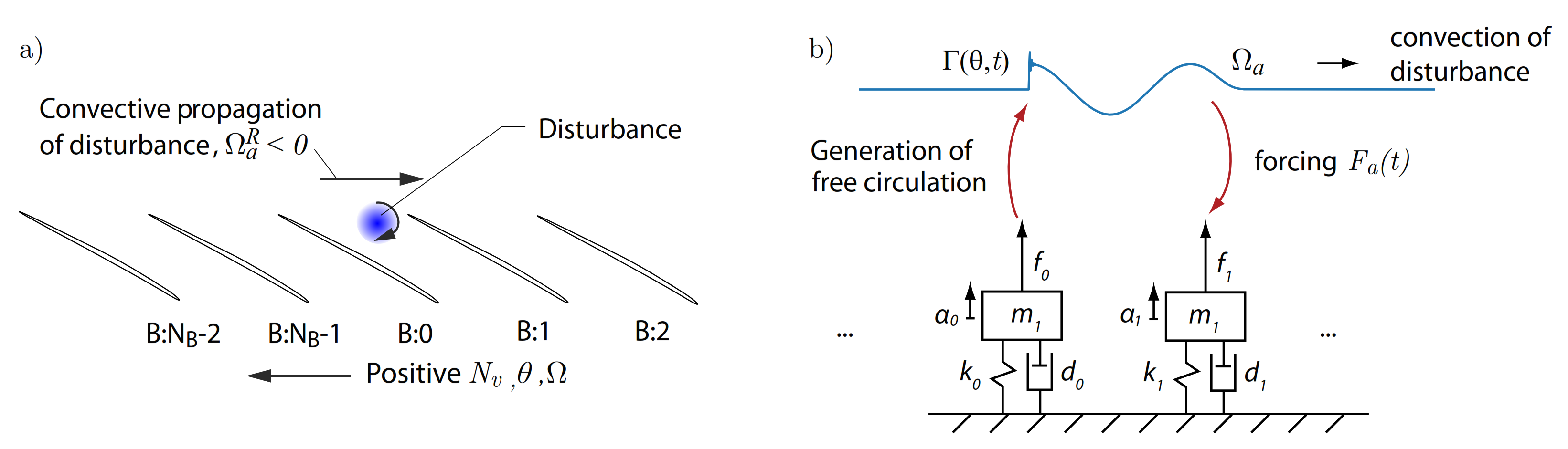
17] uses single-degree of freedom mass oscillators to represent blades on a rigid disk. In its simplest form, the individual blades are tuned and structurally uncoupled but aerodynamically coupled by a forcing term. In the case of convective NSV, the forcing is caused by a circumferentially propagating vortical disturbance. This is schematically shown in Figure 1.
It has been demonstrated that the behaviour of the 3D rotor blades undergoing torsional motion can be adequately modelled in a quasi-2D analysis, considering the twist of a spanwise section. In this case, the modal force can be approximated by the moment induced by the unsteady lift and the modal displacement q can be replaced with twist of the blade α ( α q ). If the changes in the location of the centre of pressure are negligible, the simplified equation of motion for the system becomes:
α ¨ ( t ) + D α ˙ ( t ) + K α ( t ) = c 1 L ( t )
where c 1 is a constant of proportionality between the 2D unsteady lift, L , and 3D mass-normalised modal force. D and K are the diagonal damping and stiffness matrices. respectively. As this is describing a twist motion, the modal force is a moment, but, to align with convention, we refer to it as modal force. Since the aerodynamic disturbance can be quantified in terms of convected vorticity, the modal force term on the right-hand side can be further specified. It can be considered as a superposition of the force induced directly by the blade oscillation and that caused by a circumferentially propagating vortical disturbance, which is also referred to as the aerodynamic disturbance in the following. Assuming that apparent mass effects are negligible and that the twist velocity is small compared to the inlet velocity, we can use the model of Theodorsen [18] to approximate the unsteady lift due to blade twist and the Kutta–Joukowski theorem to approximate the force induced by a travelling disturbance. This results in the following equation of motion [17]:
α ¨ ( t ) + D α ˙ ( t ) + K α ( t ) = 1 2 c 1 ρ v 2 c L ˜ α α ( t ) force due to vibration + c 1 ρ v L ˜ Γ Γ ( t ) force due to convected disturbance
where ρ is the density, v is the relative inlet velocity and c is the blade chord. The coefficient L ˜ α models the unsteady aerodynamic response of the blade. Similar to Theodorsen’s function, it is a function of the reduced frequency k and operating point, but, for simplicity, we assume a constant operating point and tuned system to drop these dependencies. In the second term on the right-hand side, L ˜ Γ is a complex constant accounting for the unsteady effects induced by the vortical disturbance Γ ( t ) . It models the change in amplitude and phase relative to the quasi-steady force.
The lift coefficient L ˜ Γ is a function of reduced frequency and blade deflection amplitude but is assumed to be constant here, since the reduced frequency is kept constant and the blade deflections are assumed to be small ( α < 2 ). The convection of circulation around the circumference, Γ ( t ) , couples the different rotor blades aerodynamically. Equation (2) clearly shows that the right-hand side of the equation of motion for the NSV problem comprises two terms: the first one models the forces induced by vibration, F v , and the second one those induced by a circumferentially travelling aerodynamic disturbance, F a :
α ¨ ( t ) + D α ˙ ( t ) + K α ( t ) = F v ( t ) + F a ( t )
At first sight, Equation (3) resembles a forced response problem, where the excitation forces F a can be linearly superimposed with the vibration forces F v . In the absence of any vibration-independent aerodynamic unsteadiness ( F a = 0 ), Equation (3) describes the flutter case. In the case of NSV, experimental measurements and simulations indicate that the aerodynamic disturbance is modified by the blade vibration [13]. Furthermore, in the computational model used to study NSV, the aerodynamic disturbance is generated by the oscillating blades ( Γ α ˙ ), such that both terms on the right-hand side depend on the blade vibration:
α ¨ ( t ) + D α ˙ ( t ) + K α ( t ) = F v ( α ( t ) ) + F a ( α ˙ ( t ) )
From Equation (4) alone, it is impossible to distinguish between NSV and flutter. In the following, we further analyse the nature of the aerodynamic forcing term F a to demonstrate that there are some key differences between the two phenomena.

3. Frequency Domain Description

In the model shown above, the aerodynamic forcing results only from the blade vibration and is linearly dependent on the blade vibration amplitude. Under some assumptions, it is possible to recast it into the frequency domain and predict stability using eigenvalue analysis.

3.1. Derivation of Influence Coefficients

To cast the system into the frequency domain, we derive an expression for the aerodynamic influence coefficients (AICs) based on the assumptions of vibrating blades and circumferentially convected aerodynamic disturbances. AICs are coefficients describing the forcing (amplitude and phase) generated by an oscillating blade on other blades in the assembly. They are normally used to determine the aerodynamic damping in all nodal diameters from a single vibrating blade, in experiments as well as simulations. Detailed explanations can be found in, for example, the work of Crawley [19].
To derive the AICs, we assume that the rotor blades are vibrating at an angular frequency ω v in the rotor frame of reference, in nodal diameter N v , such that the structural inter-blade phase-angle is given by σ v = 2 π N v / N B . The aerodynamic disturbance has circumferential propagation speed Ω a R in the rotor frame of reference. The sign convention is such that a positive circumferential direction is in the direction of rotation and therefore Ω a R < 0 , as illustrated in Figure 1. The aerodynamic disturbance is being emitted at frequency ω a in the rotor frame of reference. This could be, for example, vorticity being shed from one blade as a result of an aerodynamic instability, but it could also be due to vibration in a structural eigenfrequency ω v . Since it is difficult to induce sufficiently small variations to cause local vortex shedding in numerical simulations, the CFD simulations used to calibrate the model in [17] relied on vibration as a disturbance trigger. We therefore consider the special case where the aerodynamic disturbance is originating from the vibrating blade and ω a = ω v . Since the disturbance is generated by the blade vibration, the distinction between F v and F a is not clear (see Equation (4)). We now demonstrate why it is nevertheless necessary by deriving an expression of aerodynamic forcing on a single blade in an assembly of N B blades. For this, it is helpful to distinguish between the situation before lock-in and after lock-in.

3.1.1. Before Lock-In

To distinguish between F v and F a , we consider that it takes a finite time, namely:
T = 2 π N B Ω a R
for a disturbance emitted from a given blade at the beginning of blade vibration at t = 0 to travel one pitch. Any force experienced by the trailing blade before this is defined as F v , and the difference between the total force and the force due to blade vibration is the force due to the aerodynamic disturbance F a .
F ( t ) = F v ( t ) for t < T F v ( t ) + F a ( t ) for t T
The force due to the aerodynamic disturbance is a superposition of the forces F a , n caused by N preceding blades. Note that N here is the number of blades that have an influence on a given blade, which is not necessarily equal to N B . The force becomes:
F ( t ) = F ˜ v e i ω v R t for t < T F ˜ v e i ω v R t + n = 0 N 1 F a , n ( t ) for T < t < N T
with n counting against the direction of disturbance propagation. As defined above, in the case analysed here, the forces are periodic with frequency ω v :
F a , n = F ˜ a , n e i ω v t
We can now derive an expression for F a ( t ) in terms of the force experienced by a blade due to the oscillation of its predecessors and inter-blade phase angles.
The aerodynamic inter blade phase angle, i.e., the phase lag of the disturbance between two subsequent blades is given by:
σ a = ω v T = 2 π ω v N B Ω a R
The blades are not necessarily vibrating in phase but before lock-in the vibration can be random without a fixed inter-blade phase angle. We therefore define the vibration of individual blades through the inter-blade phase angle σ v , n :
α 0 = α ^ e i ω v t , α n = α ^ e i ω v t + σ v , n
where α ^ is the vibration amplitude, which is assumed to be constant between blades. The aerodynamic disturbance attenuates while travelling around the circumference as vorticity is not convected purely circumferentially but also axially out of the domain. Assuming an exponential decay of the disturbance, the forcing amplitude generated by the n th preceding blade is modelled as F ˜ a , n = F ˜ a * e n r a , where F ˜ a * is the complex constant representing the force caused by an immediately preceding blade. The expression for F a ( t ) becomes:
F a ( t ) = n = 0 N 1 F ˜ a * e n r a e i ( ω v t + σ v , n n σ a )
= n = 0 N 1 F ˜ a * e n r a e i ( σ v , n n σ a ) e i ω v t
It is now possible to compare this to the flutter case, where F v ( t ) = F ˜ v e i ω v R t . To do this, we set the number of preceding blades to infinity, consistent with a periodic state, and we assume vibration at a fixed inter-blade phase angle given by:
σ v , n = n 2 π N v N B = n σ v
Equation (12) then becomes:
F a ( t ) = F ˜ a * e i ω v t n = 0 e n r a e i n ( σ v + σ a ) = F ˜ a * e i ω v t 1 e r a e i ( σ v + σ a ) 1 2 e r a cos ( σ v + σ a ) + e 2 r a
where the equality k = 0 p k e i k x = [ 1 p e i x ] / [ 1 2 p cos x + p 2 ] is used. The sum of the inter-blade phase angles expressed in terms of nodal diameters and frequencies is:
σ v + σ a = 2 π N v + ω v / Ω a R N B
Two differences between convective NSV and flutter become apparent in Equations (12) and (14). There are two distinct time scales in the case of NSV: the vibration time scale and the aerodynamic, or convective, time scale, n σ a = n ω v / ( N B Ω a R ) 
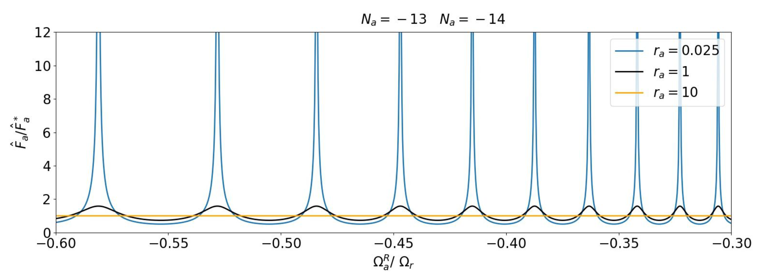
. If the convective time scale is not an integer multiple of the vibration period, the phase-lag between the aerodynamic disturbance and vibration modulates the forcing, creating a beating signal. The amplitude of this depends on the decay coefficient r a . For a given r a , the amplification in time of the force generated by the aerodynamic disturbance, which we measure here as an amplitude ratio F ^ a / F ^ a * , reaches a maximum if the frequency is in resonance with the vibration frequency, i.e., ω v R = N a Ω a R , as in a forced response function. This is shown in Figure 2, for different decay coefficients, where the amplification for a fixed vibration frequency and range of propagation speeds Ω a R was computed. However, unlike classical forced response, the aerodynamic excitation in this scenario depends on the vibration amplitude.
The other difference results from the decay coefficient r a . The value of r a determines how many blades are influenced by the vibration of a given blade. For low values of r a , it is possible that an aerodynamic disturbance originating from one blade travels around the entire circumference and returns to the original blade.

3.1.2. After Lock-In

The numerical studies in [17] showed how lock-in of the disturbance and a vibration pattern is achieved through a phase-modulation of the disturbance when it is interacting with an oscillating blade and the establishment of a nodal diameter pattern such that the phase-speed of the aerodynamic disturbance matches that of the structure. In this case, the resonance condition
ω v R = N a Ω a R where N a = { 1 , 2 , , n }
is fulfilled, i.e., an integer number of aerodynamic wave lengths fits into the circumference. Substituting Equation (16) into Equation (15), we then see that:
σ v + σ a = 2 π N v N a N B = 2 π m where m = { 1 , 2 , , n }
such that Equation (14) simplifies to:
F a ( t ) = F ˜ a * e i ω v t 1 1 e r a
Considering a case where the disturbance rapidly decays over the circumference, i.e., r a , recovers the expression for flutter:
lim r a F a ( t ) = F ˜ a * e i ω v t
In the case of r a 0 , the aerodynamic forcing amplitude diverges even in the absence of a coupled fluid–structure instability.
The above analysis examines the relationship between NSV and flutter. Equation (18) shows how, even after lock-in, when it is impossible to distinguish unsteadiness resulting from aerodynamics from that of vibration, the physics governing the system are different. In the case of NSV, the attenuation of a circumferentially propagating disturbance is low, while it is high in the case of flutter. In other words, in the case of NSV, an aerodynamic instability exists, which does not require participation of the structure. This is not the case for flutter.
To further illustrate the difference between NSV and flutter, it is useful to compare the above description to an aerodynamic influence coefficient (AIC) formulation which can then be used to analyse the stability of the system.

3.2. Comparison to Classical AIC Approach

When the number of preceding blades considered in the summation is less than the number of blades in the circumference N N B 1 , which is a valid choice for rapid decay of the aerodynamic disturbance, Equation (12) becomes:
F a ( t ) = n = 0 N 1 F ˜ a * e n r a e i [ ω v t n ( σ v + σ a ) ]
Noting that the amplitude of the force is proportional to the blade modal velocity, because vorticity is being generated by the blade oscillation [17], and including the forces resulting from vibration on the vibrating blade itself, F v ( t ) , this can be rewritten to resemble a classical aerodynamic influence coefficient formulation. In this case, the equation of motion for a given blade and inter-blade phase angle, σ v , becomes:
α ¨ + 2 ζ v ω v α ˙ + ω v 2 α = C ˜ v α + n = 0 N 1 C ˜ a , n σ v α ˙ n
where the first term on the right-hand side represents the aerodynamic influence of the blade on itself and the sum contains the contribution of all other blades. The solution for the modal displacement is assumed to be a complex exponential,
α = α ^ e λ t where λ = ω v ζ ± i ω v ω 2 ω v 2 ζ 2
such that the solution to the eigenvalue problem will give the aeroelastic frequency, ω , and aerodynamic damping, ζ . The blade influence coefficients C ˜ a , n σ v and C ˜ v relate to the aerodynamic force coefficient F ˜ a * as follows:
C ˜ a , n σ v = F ˜ a * ω v α ^ e n r a e i n ( σ v + σ a ) = C a * ˜ e n r a e i n ( σ v + σ a ) C ˜ v = F ˜ v α ^
In other words, the influence coefficient as derived from AIC simulations automatically incorporates the phase-lag and decay. It is normally obtained using CFD simulations without any knowledge of the physical mechanisms causing the aerodynamic coupling between blades. (Note that, in the typical AIC analysis, the vibration inter-blade phase angle σ v would not feature in the aerodynamic influence from Blade n to Blade 0 (as only one blade is vibrating). Instead, the complex blade-individual influence coefficient is transferred into the travelling wave space by a Fourier transform).
The comparison to the classical AIC approach clearly shows that, in a locked-in state and for a sufficiently high decay of the disturbance around the circumference, the problem is equivalent to flutter and can be analysed using aerodynamic influence coefficients. The problem in the case of NSV is how these influence coefficients are defined. Without sufficient decay, the aerodynamic disturbance would traverse the entire circumference and the coefficients would be time dependent (on the number of revolutions of the disturbance). In this case, they are impossible to obtain using CFD simulations because the AIC paradigm is that the influence decays to zero with distance from the oscillating blade. This is illustrated with examples in the following section.

4. Rotor Stability Analysis

To illustrate the use of the model, it is here applied to a transonic rotor exhibiting non-synchronous vibrations near stall in the first torsional mode. The case and experimental procedure is described in detail in [13] but is briefly reviewed here.

4.1. Test Case

The test case is a 1.5 stage research compressor representative of modern high-pressure compressor front stages. The rotor operating map is shown in Figure 3. In the experiments, high vibration amplitudes in the 1T/8ND mode were measured when the compressor was throttled from the last point shown on the map. The CFD simulations used to calibrate the model were performed using the in-house Reynolds-averaged Navier–Stokes solver AU3D. Details about the calibration process are given in the next section. Steady state simulations were performed on single-passage mixing plane models, while unsteady simulations were performed on a five-passage model of the rotor only, with the centre blade vibrating as illustrated in Figure 1. Details regarding the CFD simulations can be found in [17].
As seen in Figure 3, the steady state CFD simulations of the 1.5 stages did not reach the near-stall operating point but with simulations of the isolated rotor at increased back-pressure the stall mass flow was reached. On this rotor-only characteristic, two operating points are labelled. OP1 presents the point of maximum pressure rise in the rotor and OP2 presents the last point for which convergence in the steady simulation could be reached. Using unsteady simulations, the operating point shifts as indicated in the picture.
A validation of the CFD is shown in Figure 3, where the flow field measured at the near stall operating point is compared to CFD simulations at OP1 and OP2. The flow field at OP2 matches that of the experiment well. As a result of the tip leakage flow, the passage is almost completely blocked by low velocity fluid downstream of the shock. At this operating point, a vortical disturbance is transported predominantly in the circumferential direction. It was previously shown that this is the main contributor to forcing on the blades during NSV. In the formulation above, this corresponds to a low decay coefficient r a . At the higher mass flow operating point (OP1), the majority of the vorticity is convected axially out of the passage and r a takes a high value.

Validation of Frequency Model

The frequency domain model is now applied to the transonic rotor for the two operating points of interest. The coefficients, listed in Table 1, were previously calibrated using reduced-domain CFD simulations at OP1 and OP2, where a central blade (Blade 0) was oscillated in the torsional mode and the resulting forces on the other blades were recorded (see Figure 1). The force coefficients F ˜ a * and F ˜ v are determined from the time histories of modal forces on Blade 1 and the oscillating Blade 0, respectively, while the decay rate was found by comparing forcing amplitudes on all five blades in the domain.
Due to the low decay rate of the aerodynamic disturbance, a periodic solution does not exist at the NSV operating point (OP2), and the force coefficients are time dependent. The present analysis uses rounded values following calibration during the first few cycles of blade vibration.
Figure 4a shows the aerodynamic damping curves at the two operating points. While OP1 is stable, OP2 shows significant negative aerodynamic damping in nodal diameter N v = 8 . The associated shift in frequency of the aeroelastic system relative to the in-vacuo frequency ω v is shown in Figure 4b. This shift in frequency shows how the fluid–structure coupling modifies the phase-speed of the aerodynamic disturbance. At the unstable nodal diameter, the aerodynamic disturbance and structural vibration are close to resonance and the shift in frequency is minimal. For N v = 7 , on the other hand, the frequency shifts by 3%. This lock-in effect was also seen in the experiment and numerical simulations [13,17]. The results at OP1 (stable) and OP2 (instability at N v = 8) are in agreement with the experimental measurements and validate the frequency domain model.

4.2. Application to Cases from Literature

To test the general applicability of the model and these results, we applied it to a number of cases from the literature, as listed in Table 2. The forcing coefficients F ˜ v and F ˜ a * were not changed from the calibrated values (Table 1), but the non-dimensional vibration frequency ω v / Ω r and propagation speed Ω a R / Ω r were adjusted for each case, based on information from the literature. Using these settings, the model was able to correctly predict the unstable nodal diameter for all the cases in Table 2. This indicates that the critical (unstable) nodal diameter for a case can be correctly predicted knowing only the number of blades, frequency of vibration and propagation velocity. The former two are known, while the latter can be approximated from the swirl velocity in the leading edge plane. The model predicts the resonance condition, and as such the critical nodal diameter can also be identified using simple algebra. The interesting outcome of this experiment is that the same set of values for the coefficients F ˜ a * and F ˜ v gives good results for all cases. This implies that either all cases and their force coefficients are comparable or the amplitude and phase of the coefficients plays a minor role. The latter would imply that it is not necessary to recalibrate coefficients to assess the stability of a compressor at different operating points. The sensitivity to the coefficients is therefore studied in the following section.

5. Parametric Investigation

The influence of the decay rate, rotational speed and force coefficients on the stability of the system is now analysed. The baseline parameters are listed in Table 1, where the values are representative of those determined at OP1 and OP2.

5.1. Influence of Decay Rate

The effect of the decay rate r a on aerodynamic damping is shown above in Figure 4. The only difference between OP1 an OP2 in this analysis is the decay rate, which is another indicator that the key difference between NSV and flutter lies in the propagation behaviour of the aerodynamic disturbance. Further sensitivity studies are not shown here because a variation in r a is equivalent to including more blades in the influence coefficient sum, which is known to change the shape of the aerodynamic damping curve (Figure 4a) by adding higher harmonics as the number of blades in increased.

5.2. Influence of Propagation Speed

We continue by studying the influence of propagation speed of the aerodynamic disturbance Ω a R / Ω r = Ω a N R on aerodynamic damping. The speed was varied between 0.2 and 0.8 Ω R because this range of speeds is associated with NSV in the literature.
Figure 5 plots the least damped nodal diameter against propagation speed. It therefore shows which nodal diameter would be responding when the swirl velocity is changed, reproducing the familiar ‘stair case’ plots seen during acceleration manoeuvres or re-scheduling of inlet guide vanes (e.g., [22,23]). The size of the markers in Figure 5 corresponds to the magnitude of aerodynamic damping. To explain the trends seen here, the aerodynamic damping curves for four selected values close to the measured propagation speed are plotted in Figure 5b. At the operating speed corresponding to OP2 ( Ω a N R = 0.44 ), we see large negative aerodamping at N v = 8, indicating that the aerodynamic disturbance is in resonance with the vibration mode. When the relative speed is increased sightly to Ω a N R = 0.42 , N v = 8 is marginally unstable. A slightly lower speed ( Ω a N R = 0.46 ) still shows instability at N v = 8 but a reduced magnitude compared to the OP2 operating point.
From the results in Figure 4 and Figure 5, it is clear that fluid–structure lock-in is possible because the aerodynamic wave number and (to a smaller extent) the phase speed of the disturbance are parameters that are determined by the coupled system, such that the phase-speed of the disturbances matches that of the structure.

5.3. Influence of Amplitude and Phase of Aerodynamic Coefficients

The two aerodynamic force coefficients, F ˜ v and F ˜ a * , are taken as constants in the model. However, their magnitude and phase in reality depend on not only the geometry and operating point but also the reduced frequency. To test the sensitivity of the system’s stability on these coefficients, the phase and amplitude are varied independently. Figure 6 shows the effect of the magnitude of the force coefficients on aerodynamic damping. A change in the blade influence on itself, F ˜ v , simply shifts the damping curve, with a larger amplitude resulting in a higher mean aerodynamic damping. This is consistent with flutter in turbomachinery and shows that the blade’s influence on itself is stabilising. A change in the amplitude of the aerodynamic disturbance alters the shape of the curve, showing a larger variation between nodal diameters, N v . This is also consistent with flutter. This behaviour is much more noticeable at OP1 than at OP2. While at OP1 the mean damping is comparable to its variation, damping at OP2 is dominated by the contribution from the aerodynamic disturbance and damping values are an order of magnitude larger than at OP1.
The phase of the vibration-associated coefficient F ˜ v has a similar effect as its amplitude and influences the mean aerodynamic damping as expected (see Figure 7). The phase of the force induced by the aerodynamic disturbance F ˜ a * has a significant effect at OP1. A small shift in the response of the blade results in a shift of minimum aerodynamic damping to another nodal diameter. At OP2, the shift in phase reduces the magnitude of negative damping but does not change the nodal diameter of the instability.

6. Discussion

The analysis and application showed that the linear model developed for convective NSV can predict the correct vibration mode, and that the results depend significantly on the disturbance attenuation over the circumference, which is determined by the blockage in the tip region and therefore depends on the operating point. The model as developed above relies on a number of assumptions, namely:
  • The forcing due to multiple disturbances can be linearly superposed.
  • The amplitude of the aerodynamic disturbance and therefore the forcing coefficient, F ˜ a , 0 , depend linearly on vibration amplitude.
  • The forcing coefficient F ˜ a , 0 does not change with blade oscillation phase.
  • All blades are aerodynamically and structurally identical.
While the last one is valid for a tuned bladed disk or blisk, the first three need to be improved to allow quantitative predictions of the vibration amplitudes. Parameter studies [17] have shown that the forcing coefficient behaves non-linearly at high vibration amplitudes and varies with phase. Similarly, the disturbance becomes saturated, which makes it possible for the compressor to operate aerodynamically stable at the NSV operating point.

7. Conclusions

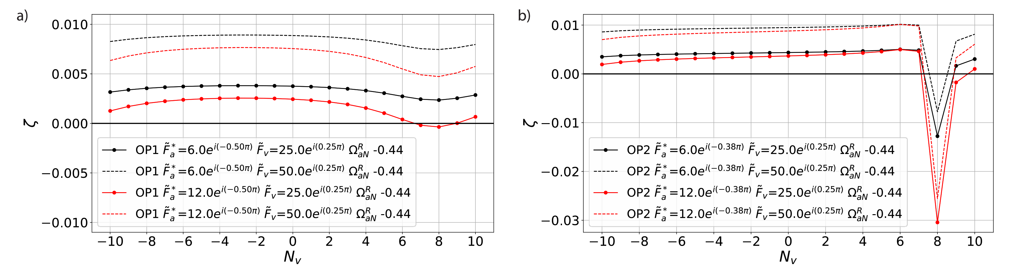
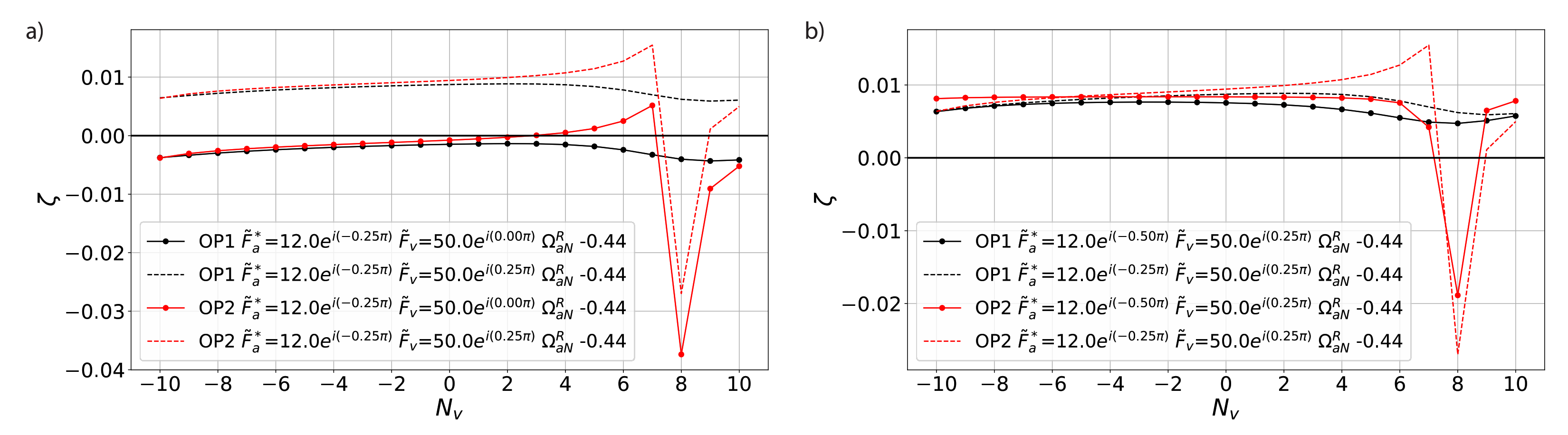
This paper derives aerodynamic influence coefficients for compressor non-synchronous vibrations near the stall boundary, which are caused by the circumferential propagation of a vorticity disturbance. The influence coefficients are used in a linear frequency-domain model to predict the stability of the aeroelastic system. Unlike classical AICs, the present influence coefficients are derived from physical principles and are functions of the system’s structural and aerodynamic properties. This makes it possible to study the sensitivity of NSV to parameters such as propagation speed and circumferential decay rate of the disturbance. It is shown that the model correctly predicts the experimentally measured unstable nodal diameters when calibrated with unsteady CFD simulations.
The results and comparison of the AIC formulation to that for flutter demonstrate that the phenomenon described is distinct from flutter. In the case of convective NSV, the system becomes unstable because an aerodynamic disturbance propagates circumferentially with little attenuation. The result is an instability which locks-in with the structural vibration frequency. In reality, the aerodynamic and aeroelastic behaviour becomes non-linear at large amplitudes, limiting aerodynamic disturbance and blade oscillation amplitudes. The modifications necessary to model this non-linearity are identified in this paper.

Author Contributions

C.B. and S.S.: Conceptualization, methodology, investigation and writing. Both authors have read and agreed to the published version of the manuscript.

Funding

The presented research was supported through Clean Sky 2 Joint Undertaking (JU), project CATANA under grant agreement N°864719. The JU receives support from the European Union’s Horizon 2020 research and innovation programme and the Clean Sky 2 JU members other than the Union. This publication reflects only the author’s view and the JU is not responsible for any use that may be made of the information it contains. The authors thank EPSRC for the support under the Prosperity Partnership Grant “Cornerstone: Mechanical Engineering Science to Enable Aero Propulsion Futures”, Grant Ref: EP/R004951/1.

Data Availability Statement

Not applicable.

Acknowledgments

We would like to thank Roque Corral of Universidad Politécnica de Madrid, Bob Kielb and Ken Hall of Duke University, and Xavier Ottavy of Ecole Centrale de Lyon for interesting discussions which inspired this work.

Conflicts of Interest

The authors declare no conflict of interest.

References

  1. Sisto, F. Introduction and Overview, AGARD Manual on Aeroelasticity in Axial-Flow Turbomachines. Volume 1. Unsteady Turbomachinery Aerodynamics; Technical Report; Advisory Group for Aerospace Research and Development: Neuilly-sur-Seine, France, 1987. [Google Scholar]
  2. Sisto, F. Stall-flutter in cascades. J. Aeronaut. Sci. 1953, 20, 598–604. [Google Scholar] [CrossRef]
  3. Emmons, H. Compressor surge and stall propagation. Trans. ASME 1955, 77, 455–467. [Google Scholar]
  4. Armstrong, E.; Stevenson, R. Some practical aspects of compressor blade vibration. Aeronaut. J. 1960, 64, 117–130. [Google Scholar] [CrossRef]
  5. Kielb, R.E.; Barter, J.W.; Thomas, J.P.; Hall, K.C. Blade Excitation by Aerodynamic Instabilities: A Compressor Blade Study. In Proceedings of the ASME Turbo Expo 2003, Atlanta, GA, USA, 16–19 June 2003; pp. 399–406. [Google Scholar]
  6. Carter, A.; Kilpatrick, D. Self-excited vibration of axial-flow compressor blades. Proc. Inst. Mech. Eng. 1957, 171, 245–281. [Google Scholar] [CrossRef]
  7. Corral, R. Bladed Disks: Flutter. VKI-LS Struct. Des. Aircr. Engines 2012, 6, RTO-EN-VT-207. Available online: https://www.sto.nato.int/publications/STO%20Educational%20Notes/RTO-EN-AVT-207/EN-AVT-207-06.pdf (accessed on 2 July 2021).
  8. Duquesne, P.; Rendu, Q.; Aubert, S.; Ferrand, P. Choke flutter instability sources tracking with linearized calculations. Int. J. Numer. Methods Heat Fluid Flow 2019, 30, 4155–4166. [Google Scholar] [CrossRef]
  9. Baumgartner, M.; Kameier, F.; Hourmouziadis, J. Non-engine order blade vibration in a high pressure compressor. In Proceedings of the Twelfth International Symposium on Airbreathing Engines, Melbourne, Australia, 10–15 September 1995. [Google Scholar]
  10. Brandstetter, C.; Ottavy, X.; Stapelfeldt, S. Interpretation of stall precursor signatures. J. Turbomach 2021. [Google Scholar] [CrossRef]
  11. Vo, H.D.; Tan, C.S.; Greitzer, E.M. Criteria for Spike Initiated Rotating Stall. J. Turbomach. 2008, 130, 11023–11029. [Google Scholar] [CrossRef]
  12. Vo, H.D. Role of tip clearance flow in rotating instabilities and nonsynchronous vibrations. J. Propul. Power 2010, 26, 556–561. [Google Scholar] [CrossRef]
  13. Brandstetter, C.; Juengst, M.; Schiffer, H.P. Measurements of Radial Vortices, Spill Forward, and Vortex Breakdown in a Transonic Compressor. J. Turbomach. 2018, 140, 061004. [Google Scholar] [CrossRef]
  14. Inoue, M.; Kuroumaru, M.; Tanino, T.; Furukawa, M. Propagation of Multiple Short-Length-Scale Stall Cells in an Axial Compressor Rotor. J. Turbomach. 2000, 122, 45–54. [Google Scholar] [CrossRef]
  15. Young, A.; Day, I.; Pullan, G. Stall Warning by Blade Pressure Signature Analysis. J. Turbomach. 2013, 135, 11033. [Google Scholar] [CrossRef]
  16. Pullan, G.; Young, A.M.; Day, I.J.; Greitzer, E.M.; Spakovszky, Z.S. Origins and Structure of Spike-Type Rotating Stall. J. Turbomach. 2015, 137, 51007–51011. [Google Scholar] [CrossRef]
  17. Stapelfeldt, S.; Brandstetter, C. Non-synchronous vibration in axial compressors: Lock-in mechanism and semi-analytical model. J. Sound Vib. 2020, 488, 115649. [Google Scholar] [CrossRef]
  18. Theodorsen, T. General Theory of Aerodynamic Instability and the Mechanism of Flutter; NACA Technical Report 496; National Aeronautics and Space Administration: Washington, DC, USA, 1949. [Google Scholar]
  19. Crawley, E. Aeroelastic formulation for tuned and mistuned rotors. In AGARD Manual on Aeroelasticity in Axial-Flow Turbomachines; Structural Dynamics and Aeroelasticity, AGARDograph No. 298; AGARD: Neuilly sur Seine, France, 1988; Volume 2, Available online: https://www.sto.nato.int/publications/AGARD/AGARD-AG-298-VOL-2/AGARD-AG-298-Vol-2.pdf (accessed on 2 July 2021).
  20. Kameier, F.; Neise, W. Rotating Blade Flow Instability as a Source of Noise in Axial Turbomachines. J. Sound Vib. 1997, 203, 833–853. [Google Scholar] [CrossRef]
  21. Rodrigues, M.; Soulat, L.; Paoletti, B.; Ottavy, X.; Brandstetter, C. Aerodynamic investigation of a composite low-speed fan for UHBR application. In Proceedings of the ASME Turbo Expo 2020: Turbomachinery Technical Conference and Exposition, London, UK, 22–26 June 2020. [Google Scholar]
  22. Franke, D.; Jüngst, M.; Möller, D.; Schiffer, H.P.; Giersch, T. Influence of Pre-swirl, Rotor Speed and Blade Count on Aeroelastic Coupling Mechanisms during Stall Inception of a Transonic Compressor. In Proceedings of the ASME Turbo Expo 2020: Turbomachinery Technical Conference and Exposition, London, UK, 22–26 June 2020. [Google Scholar]
  23. Dodds, J.; Vahdati, M. Rotating Stall Observations in a High Speed Compressor—Part I: Experimental Study. J. Turbomach. 2015, 137, 51002–51010. [Google Scholar] [CrossRef]
Figure 1. (a) Sketch of rotor indicating blade numbering and sign convention and propagation of disturbance and (b) schematic of the model.
Ijtpp 06 00026 g001
Figure 2. Amplification of disturbance for different decay coefficients.
Ijtpp 06 00026 g002
Figure 3. Constant-speed characteristic and flow field at 92% span.
Ijtpp 06 00026 g003
Figure 4. Aerodynamic damping (a) and aeroelastic frequency ratio (b) versus nodal diameter for the experimentally tested operating points.
Ijtpp 06 00026 g004
Figure 5. (a) Critical (unstable) nodal diameter as function of propagation speed. Symbol size proportional to amplitude of ζ . (b) Damping coefficient for variation of propagation speed.
Ijtpp 06 00026 g005
Figure 6. (a) OP1 and (b) OP2, variation of amplitude F ˜ a * and F ˜ v .
Ijtpp 06 00026 g006
Figure 7. (a) Variation of phase of F ˜ v and (b) variation of phase of F ˜ a * .
Ijtpp 06 00026 g007
Table 1. Coefficients and parameters used to represent OP1 and OP2.
OP1OP2
Decay rate, r a 1.0 0.075
Propagation speed, Ω a N R = Ω a R / Ω r R 0.44 0.44
Force coefficient F ˜ a * = C ˜ a * α ^ 12 e i ( 0.50 π ) 12 e i ( 0.375 π )
Force coefficient F ˜ v = C ˜ v α ^ 50 e i ( 0.25 π ) 50 e i ( 0.25 π )
Number of blades N B 2121
Vibration frequency ω v R / Ω r 5.81 5.81
Table 2. Cases from the literature successfully captured by the model, listing model inputs (number of blades, propagation speed and vibration frequency), experimentally measured nodal diameter N v , e x p and nodal diameter predicted by the reduced order model N v , m o d e l .
N B Ω a R / Ω r ω v / Ω r σ v , exp N v , exp N v , model
Baumgartner et al. [9]27 0.36 7.56 80 66
Kameier and Neise [20]24 0.6 22.2 165 1111
Brandstetter et al. [13]21 0.44 5.8 137 88
Rodrigues et al. [21]16 0.42 5.46 67.5 33
Publisher’s Note: MDPI stays neutral with regard to jurisdictional claims in published maps and institutional affiliations.

