Numerical Prediction of the Aerodynamics and Acoustics of a Tip Leakage Flow Using Large-Eddy Simulation ^†

Abstract

A Large-Eddy Simulation of the tip leakage flow of a single airfoil is carried out. The configuration consists of a non-rotating, isolated airfoil between two horizontal plates with a gap of 10 mm between the tip of the airfoil and the lower plate. The Mach number of the incoming flow is 0.2, and the Reynolds number based on the chord is 9.3 × 10${}^5$. The objective of the present study is to investigate the best way to compute both the aerodynamics and acoustics of the tip leakage flow. In particular, the importance of the inflow conditions on the prediction of the tip leakage vortex and the airfoil loading is underlined. On the other hand, the complex structure of the tip leakage vortex and its convection along the airfoil was recovered due to the use of a mesh adaptation based on the dissipation of the kinetic energy. Finally, the ability of the wall law to model the flow in the tip leakage flow region was proven in terms of wall pressure fluctuations and acoustics in the far-field.

1. Introduction

Due to strong environmental constraints regarding the noise emitted by aircraft, the bypass ratio of modern turbofan engines has tended to increase. This ratio is associated with a reduction of the fan rotation speed, the exhaust jet speed, and possibly the nacelle length. When looking at the noise sources of an engine at the approach regime, the fan stage is one of the major contributors. In this context, the understanding and prediction of secondary noise sources, such as the tip clearance noise in the fan stage, is required.

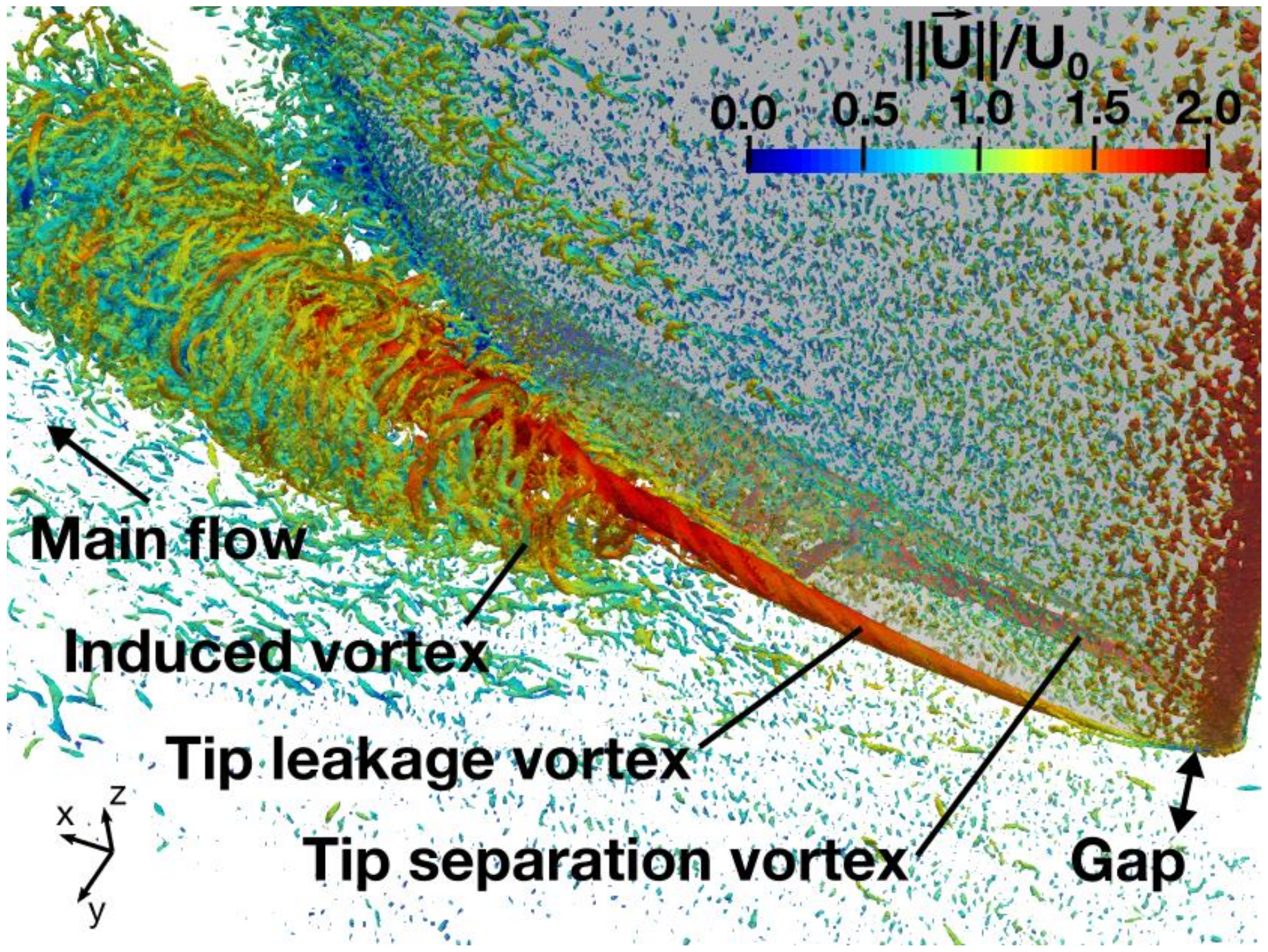
In the fan stage of turbofan engines, a gap between the tip of fan blades and the casing wall is present. As a consequence, a highly three-dimensional unsteady secondary flow develops. The tip leakage flow goes from the pressure side to the suction side of the blade. When the tip leakage flow leaves the gap, it interacts with the primary flow and rolls up to form the tip leakage vortex. The aerodynamic phenomena are mainly controlled by the blade tip loading, gap height, blade tip thickness, stagger angle, and Reynolds and Mach numbers. The consequences of a too strong gap are a drop in the aerodynamic fan performance and an increase in radiated far field noise [1].

This increase of the radiated noise from axial fans was first observed experimentally when the height of the gap increased [2]. Then, source mechanisms responsible for tip clearance noise generation were investigated. First, Kameier and Neise [3] identified a component of the tip clearance noise called the rotating instability. This mechanism consists of coherent vortical structures coming from the tip clearance that interact with the fan blades, causing periodic fluctuations of the blade loading, and thus inducing tonal noise in the far field. Yet, as these vortices have a range of tangential velocities, broadband humps are observed instead of sharp tonal peaks. This mechanism appears at off-design conditions, close to the rotating stall, and the structure of the tip clearance flow region is completely changed. Secondly, Fukano et al. [4] studied the tip clearance self noise. The periodic velocity fluctuations generated by the wandering of the tip leakage vortex produce tonal noise. Simultaneously, a broadband noise due to the enhancement of stochastic velocity fluctuations in the blade passage is generated. Previous observations were more detailed in the experiment of Jacob et al. [5]. Indeed, the authors described the vortical structures generated by the tip leakage flow and observed that they were scattered as sound by the edges of the tip trailing-edge corner, acting as dipole sources. Moreover, they described the jet-like leakage flow as another component of the tip clearance noise with the characteristic of a quadrupole noise source.

Various numerical studies were performed to investigate the tip clearance noise. An Unsteady Reynolds-Averaged Navier-Stokes (URANS) simulation of a rotor was achieved by März et al. [6] to confirm the experimentally-observed phenomena of rotating instability and to interrogate the physical mechanism behind it. Then, Zhu et al. [7] used unsteady aeroacoustic predictions with the Lattice Boltzmann Method (LBM) to shed more light on this noise generation mechanism. Moreover, Boudet et al. [8] achieved a Zonal Large-Eddy Simulation (ZLES) of a fan rotor where the region of interest at the tip was simulated with full Large Eddy Simulation (LES), and the hub and midspan regions were simulated with Reynolds-Averaged Navier–Stokes (RANS). This allowed them to identify a tip leakage vortex that was wandering and producing tonal noise. An isolated fixed airfoil with a gap designed to study the tip clearance noise self noise is considered in this paper. ZLES [9], LES [10], and LBM [11] approaches were achieved on this configuration.

The isolated non-rotating airfoil is mounted in an open-jet wind-tunnel facility. This experimental environment is tough to reproduce numerically due to the strong interaction between the jet and the airfoil. Indeed, when testing a lifting airfoil, the main stream is deflected by the equivalent lateral momentum injection, which reduces the effective angle of attack. The flow around an airfoil when installed in a free-jet wind tunnel significantly deviates from that of the same airfoil placed in a uniform stream. A solution to compute the airfoil in an uniform flow is to modify the angle of attack to retrieve the proper airfoil loading. Although the integrated lift can be adjusted in this way, the precise distribution of pressure coefficient is not perfectly recovered. As proposed by Moreau et al. [12], one way is to impose a more realistic inlet boundary condition from a precursor RANS calculation. The other way is to account for the full experiment set-up.

The objective of the present study is to investigate the best way to compute both the aerodynamics and acoustics of the tip leakage flow in order to transfer the methodology to real turbomachinery configurations. To do so, we simulated the same experimental set-up using two different computational domains, including modelling the inflow conditions, with a predictive LES approach. The use of a wall model, synthetic-turbulence injection and adaptive mesh refinement are also considered.

The paper starts with a description of the experimental set-up. Then, the numerical set for each configuration is detailed in the second section. In the third section, LES results for the two different computational domain approaches are compared and discussed. Next, the effect of mesh refinement on the prediction of the tip leakage vortex is shown. Finally, the ability of the wall law to model the boundary layer in the gap region is analysed, as well as its impact on the acoustic radiation. Concluding remarks and perspectives are also given in the last section.

2. Experimental Set-Up

The numerical study is based on the isolated non-rotating airfoil experiment conducted by Jacob et al. [13]. Indeed, the advantage is that the tip clearance noise contribution to the far field noise is more easily isolated than in a rotating turbomachinery configuration. A sketch of the experimental set-up is shown in Figure 1. A fixed single airfoil is mounted between two flat plates with a tunable gap between the lower plate and the airfoil tip. Air is coming from a rectangular nozzle. To ensure a uniform flow, the isolated airfoil is placed into the potential core of the rectangular freejet.

The airfoil is a NACA 5510 of chord c = 200 mm. The geometrical angle of attack is $\beta$ = 16.5${}^{\circ }$. The gap height is s = 10 mm. The mean flow velocity at the exit nozzle is U${}_0$ = 70 m/s, corresponding to a Mach number Ma = 0.20 and a Reynolds number based on the chord Re = U${}_0$.c/$\nu$ = $9.3\times {10}^5$. One chord upstream of the airfoil, the boundary layer thickness on the plate is 6.2 mm. The experiment was carried out under ambient pressure p${}_a$ = 97,700 Pa and ambient temperature T${}_a$ = 290 K.

The coordinate system $(O,\overrightarrow{x},\overrightarrow{y},\overrightarrow{z})$ used in this study is depicted in Figure 1. The origin, defined at the trailing edge-tip corner, is more appropriate to study the tip leakage vortex. The $\overrightarrow{x}$ axis is in the streamwise direction. The $\overrightarrow{y}$ axis is in the cross-stream direction, from pressure side to suction side. The $\overrightarrow{z}$ axis is in the spanwise direction, from the lower to the upper plate.

3. Numerical Settings

The simulations performed in this study are based on the LES methodology developed at CERFACS [14,15]. LES are performed using AVBP, an explicit, unstructured, massively parallel solver [16] which solves the compressible Navier–Stokes equations. The package pyhip [17] to handle unstructured computational grids and their associated datasets is used in combination with the antares [18] pre-postprocessing library. In this paper, each LES is performed using the same following set-up. The convective fluxes are computed using the Two-Step Taylor-Galerkin C (TTGC) finite element scheme [19]. This scheme is third-order accurate in time and space. The viscous fluxes are computed using the $2\Delta$ diffusion operator from Colin [20]. Finally, the closure of the LES equations is done using the SIGMA subgrid scale model from Nicoud et al. [21]. Regarding the boundary condition, each simulation shares the wall modelling approach and the outlet boundary modelling: a wall law [22] is applied on each wall, and a characteristic boundary condition (NSCBC) based on static pressure is applied at outlet [23]. The inlet boundary conditions are detailed below.

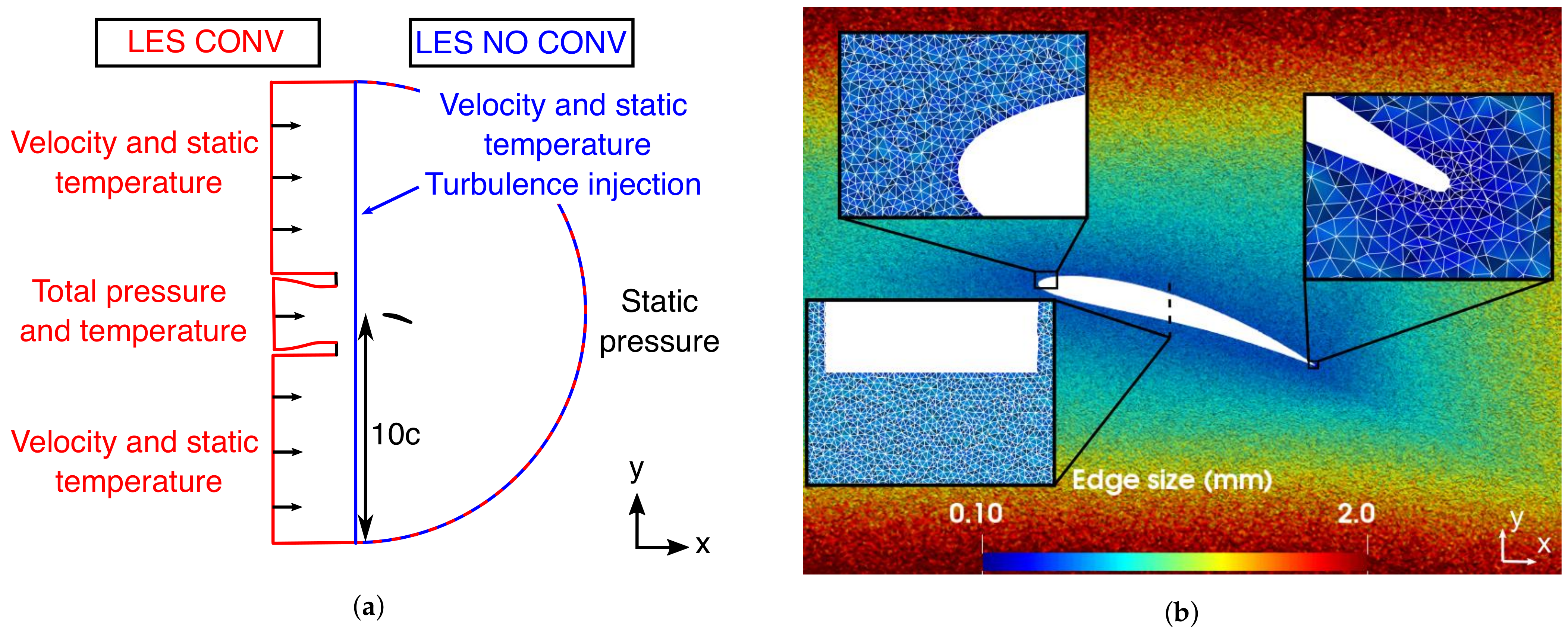
In order to define the best approach to correctly predict the airfoil flow-field, tip-leakage vortex, and associated acoustics, we chose to compare the full experimental set-up, including the convergent of the open-jet (see Figure 1) with a case where the inlet condition is imposed from a RANS simulation that included a convergent. The computational domains and the boundary conditions are summed up in Figure 2a. The simulation, including the convergent, is referred to as ’LES CONV’. In this case, the total pressure and temperature are imposed at the inlet of the convergent using a dedicated NSCBC [24]. On either side of the nozzle, a colinear flow of 1% of the jet velocity U${}_0$ (0.7 m/s) is imposed. No synthetic turbulence is injected in this case at inlet.

In the second LES (referred to as ’LES NO CONV’), in order to save CPU time, the inlet is placed one chord upstream the airfoil leading edge (the blue line in Figure 2a). The mean velocity field and static temperature are specified from a RANS computation [25]. A fully non-reflecting inlet boundary condition is used to inject three-dimensional turbulence while still being non-reflecting for outgoing acoustic waves [26]. The injected synthetic turbulence that is required to trigger the mixing layers is based on Kraichan’s method [27]. The turbulence spectrum has a Passot-Pouquet expression [28]. The Root-Mean-Square (RMS) velocity of the injected turbulent field is the one from the RANS simulation, and its most energetic turbulent length scale L${}_e$ is 6.3 mm. The latter is computed using a property of the Passot-Pouquet spectrum (L${}_e$=$\sqrt{2\pi }$L${}_t$) and the measured integral length scale L${}_t$ (2.5 mm).

In each case, the edge size of the mesh around the airfoil is unchanged as depicted with close-ups in Figure 2b. The mesh sizes at the wall of the lower plate and the airfoil are $\Delta x^{+}$ = $\Delta y^{+}$ = $\Delta z^{+}$< 100 in wall units. 20 elements are used to discretise the gap. The total number of tetrahedrons of is $229\times {10}^6$ for the case without convergent, whereas it is $252\times {10}^6$ with it. The fixed time-step is 3.5 × 10${}^{-5}$ c/U${}_0$ corresponding to a CFL number of 0.82. In each case, a computational time of $T_{ini}=7c/U_0$ is required to leave the transient state. The convergence is monitored with pressure probes in the incoming flow, in the tip leakage vortex and on the airfoil. A total of 4096 processors during 70 h were used to acquire statistics over $T_{sim}=14c/U_0$. For the same simulated time, the computational cost is increased by 20% when adding the convergent. All calculations were performed on the Joliot–Curie supercomputer in production in CEA’s Very Large Computing Centre (TGCC).

Table 1. Simulation parameters, time and cost of the two computational domain approaches.

	LES NO CONV	LES CONV
Mesh size	$229\times {10}^6$	$252\times {10}^6$
Wall resolution $\Delta x^{+}$ = $\Delta y^{+}$ = $\Delta z^{+}$	100	100
Wall model	yes	yes
Convective scheme	TTGC	TTGC
Subgrid scale model	SIGMA	SIGMA
$\Delta$t c/U${}_0$	3.5 × 10${}^{-5}$	3.5 × 10${}^{-5}$
T${}_{sim}$ c/U${}_0$	14	14
CPU time	70 h	84 h

summarizes the simulation parameters as well as the simulation time and cost. In the following, probe data were sampled at 0.01 ms leading to a LES cut-off frequency of 50 kHz. Welch’s method was used to compute Power Spectral Density (PSD) using 10 Hanning windows with an overlap of 50%. Instantaneous quantities on the airfoil surfaces are dumped every 0.025 ms leading to a cut-off frequency of 20 kHz.

4. Effects of Inflow Conditions

4.1. Instantaneous Flow

In order to have a global view of the flow field in the zone of interest, Figure 3 shows instantaneous iso-surfaces of Q criterion (Q = 3.0 × 10${}^2$ (U${}_0$/c)${}^2$) coloured by the velocity magnitude in the tip leakage flow region for the LES CONV case. As the instantaneous flow looks very similar in the LES NO CONV case, it is not shown here. The airfoil is seen from the suction side. Three vortices are identified. The tip separation vortex in the gap is generated by the separation of the tip leakage flow from the airfoil tip. The tip leakage vortex developing from the airfoil leading edge is the major one. Next to it, an induced vortex is generated by the important circulation of the tip leakage vortex. The last two vortices are contra-rotating to each other.

Figure 4 shows the instantaneous vorticity and dilatation fields in both cases at z/c = 0.1. Large differences are observed between the two approaches. First, in the vorticity field, while the tip leakage vortex (x/c >−0.5, 0 < y/c < 0.5) and the airfoil wake are similar between the two cases, the mixing layers starting from y/c = −1.0 and 1.3 are different. Indeed, considering the full experimental setup with the convergent seems to lead to a more natural growth of the jet mixing layers (Figure 4a) than with the ’LES NO CONV’ case in Figure 4b.

Secondly, when considering the acoustic field represented by the dilation field, the case without the nozzle is polluted by a strong numerical spurious noise coming from the inlet. The two sources seem to be located on the jet mixing layers and generated by the interaction of the injected turbulence and the non-constant inflow condition imposed (mean and turbulent velocity fields from RANS).

4.2. Mean Flow

The mean velocity magnitude is presented in Figure 5. The two mixing layers developed from the convergent exit section of LES CONV (Figure 5a) and from the inlet of LES NO CONV (Figure 5b) are observed as well as their deviation. Indeed, when the rectangular jet reaches the airfoil leading edge at x/c = −1, it is deflected about 8${}^{\circ }$ by the circulation generated by the airfoil. Lobes of velocity around the airfoil interact with the mixing layers at x/c = −0.5, y/c = ±1 in both cases.

However, the mixing layer development and tip leakage vortex signature differ. Indeed, as mentioned before, the mixing layers exhibit a larger growth with the add of the convergent (Figure 5a), whereas their thickness in the LES NO CONV case (Figure 5b) seems to remain constant. Regarding the tip leakage vortex flow region, a deficit of velocity magnitude is observed at y/c = 0.25, from x/c = 0 in both cases. This corresponds to the trajectory of the tip leakage vortex. Whereas the structure of the tip leakage vortex looks similar with and without the convergent, the deficit of velocity magnitude is amplified without the convergent.

The pressure coefficients on the airfoil presented in Figure 6 are similar in both cases to the measured ones (in circles) at midspan (Figure 6a) and at the tip (Figure 6b). The LES without the convergent is a blue solid line, whereas the LES with the convergent is in red. The following definition of pressure coefficient is used:

$$C_p=\frac{p-p_0}{0.5{\rho }_0{U}_0^2}$$

(1)

At midspan (Figure 6a), the LES without the convergent globally matches the experiment. The operating point of the simulation is then validated. A slight deviation is observed on the suction side, close to the leading edge (upper line for x/(c.$cos(\beta$)) <−0.8). The prediction in this region is improved by adding the convergent, while the rest of the airfoil surface exhibits the same level of pressure between the two cases.

At the tip (Figure 6b), the measured airfoil loading is globally reduced compared to the one at midspan. Indeed, the tip leakage flow from the pressure side to the suction side partially balances the pressure difference. Again, the two computed cases are able to properly predict the pressure distribution at tip which is a key point of validation. Indeed, the airfoil tip loading is one of the main parameters that control the tip leakage flow. For −0.5 < x/(c.$cos(\beta$)) <−0.2 on the suction side, a difference in the level of pressure was observed between the two LES. Unfortunately, no measurement was performed in this area. Further explanations will be given to understand the difference.

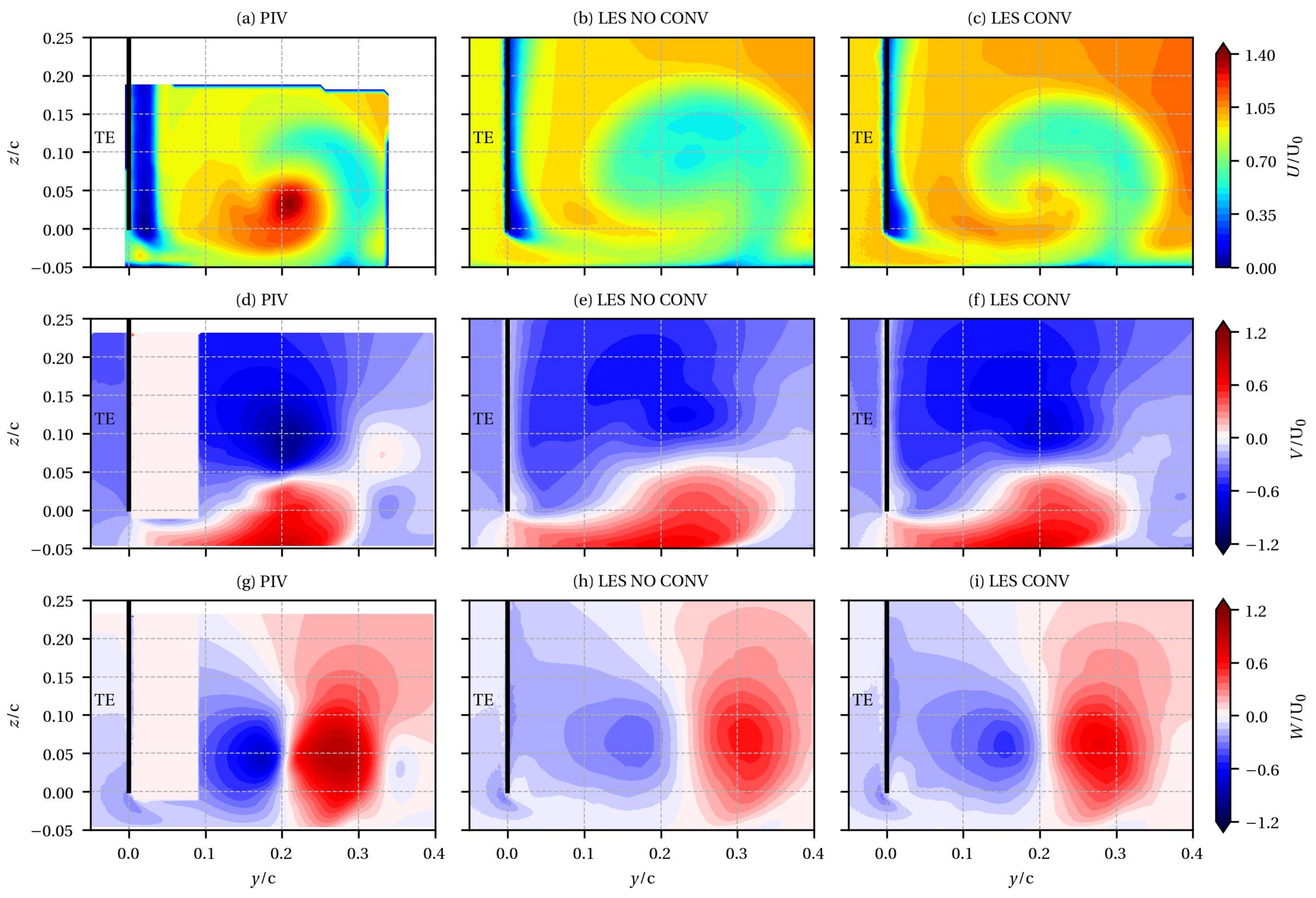
5. Tip Leakage Vortex Trajectory

Figure 7 shows the streamwise U, horizontal V and vertical W mean velocity components of the tip leakage vortex at the airfoil trailing edge (x/c = 0.01), from top to bottom, respectively. LES with and without the convergent are compared with 3D Particle Image Velocimetry (PIV) performed by Jacob et al. [13]. Since the tip leakage vortex is roughly aligned with the $\mathit{x}$ axis, the considered plane is almost perpendicular to the trajectory of the tip leakage vortex. The flow is viewed from downstream. The velocity components are normalised by the reference mean velocity U${}_0$. The airfoil trailing edge is plotted in a black solid line at y/c = 0. The white rectangle (0.0 < y/c < 0.1) in Figure 7d,g defines the airfoil projected surface as seen from the camera; however, it has no physical meaning in terms of velocity since the signal in this region is disrupted by light reflections [13].

When looking at the mean axial velocity component U of the tip leakage vortex from the PIV data (Figure 7a), two distinct regions are identified. First, a strong acceleration region with a maximum of 1.4U${}_0$ is measured at y/c = 0.22 and z/c = 0.04. This position corresponds to the centre of the tip leakage vortex. Secondly, a low velocity region surrounding the zone of acceleration extends from the plate until z/c = 0.15. The latter is generated by the detachment of the plate boundary layer by the tip leakage flow.

In both cases, LES predicts a topology that is different from the experiment but tends to recover the two regions. We observed that the LES with convergent captures better the acceleration, meaning that the incoming flow is more realistic. Nevertheless, the velocity magnitudes are lower than the measured ones. Indeed, in the LES NO CONV, the longitudinal velocity component at the centre of the tip leakage vortex is underestimated by $50\%$ compared with experiment. When adding the convergent, the difference is about $21\%$. This underprediction is attributed to the mesh resolution and will be discussed later.

Looking at the PIV measurements in Figure 7d,g, a region of positive V is observed for z/c < 0.05, whereas a region of negative V is shown for z/c > 0.05. For the vertical mean component W, two regions are also identified: positive W for y/c > 0.2 and negative W for y/c < 0.2. This clearly shows the roll up of the tip leakage vortex. The same kind of flow topology is noticeable around y/c = 0.35 but with a smaller spatial extension and opposite signs compared to the tip leakage vortex. This flow topology indicates an induced vortex. In addition, for the horizontal component V, the extension of the region in red in the gap (z/c < 0) brings out the tip leakage flow that feeds the vortex.

The LES without the convergent, in Figure 7e,h, correctly reproduces the topology of the tip leakage flow region but diffusion is noted. Indeed, a lower velocity magnitude is observed, and the tip leakage vortex is much more spatially spread out compared to the PIV. This is even more pronounced for the vertical component W. The LES with convergent in Figure 7f,i also reproduces the topology of the tip leakage vortex with an improvement on the position of the vortex. On the PIV data, the y position of the tip leakage vortex, which is identified by the sudden change of sign on W, is y/c = 0.2. While the LES without the convergent predicts the vortex at y/c = 0.23, adding the convergent allows obtaining the correct y position of the vortex. A slight improvement is also observed on the z position.

In order to quantify more precisely the tip leakage vortex trajectory, a vortex identification method developed by Graftieux et al. [29] was applied. This method is based on the function ${\mathsf{\Gamma }}_1$ derived from the velocity field. This function is able to characterise the locations of the large-scale vortex centres, by considering only the topology of the velocity field and not its magnitude.

The function ${\mathsf{\Gamma }}_1$ is defined as

$${\mathsf{\Gamma }}_1\left(P\right)={\displaystyle \frac{1}{S}}{\int }_{M\in S}{\displaystyle \frac{\left(\mathbf{PM}\wedge {\mathbf{U}}_{\mathbf{M}}\right)·\mathbf{n}}{\Vert \mathbf{PM}\Vert ·\Vert {\mathbf{U}}_{\mathbf{M}}\Vert }}dS$$

(2)

where S is a surface surrounding P, M lies in S, and $\mathbf{n}$ is the unit vector normal to S. ${\mathbf{U}}_{\mathbf{M}}$ is the velocity vector at M, and $\mathbf{PM}$ is the distance vector between P and M. ${\mathsf{\Gamma }}_1$ is dimensionless and ${\mathsf{\Gamma }}_1\in [-1,1]$. ${\mathsf{\Gamma }}_1$ may be interpreted as the normalized angular momentum of the velocity field. The sign of ${\mathsf{\Gamma }}_1$ defines the rotation sign of the vortex. ${\mathsf{\Gamma }}_1>1$ is for clockwise rotation, whereas ${\mathsf{\Gamma }}_1<1$ is for counterclockwise rotation. The centre of the vortex is defined as the maximum of $\mid {\mathsf{\Gamma }}_1\mid$ with a pragmatic threshold value at 0.9 for validity. The integration over the surface S plays the role of a spatial filter.

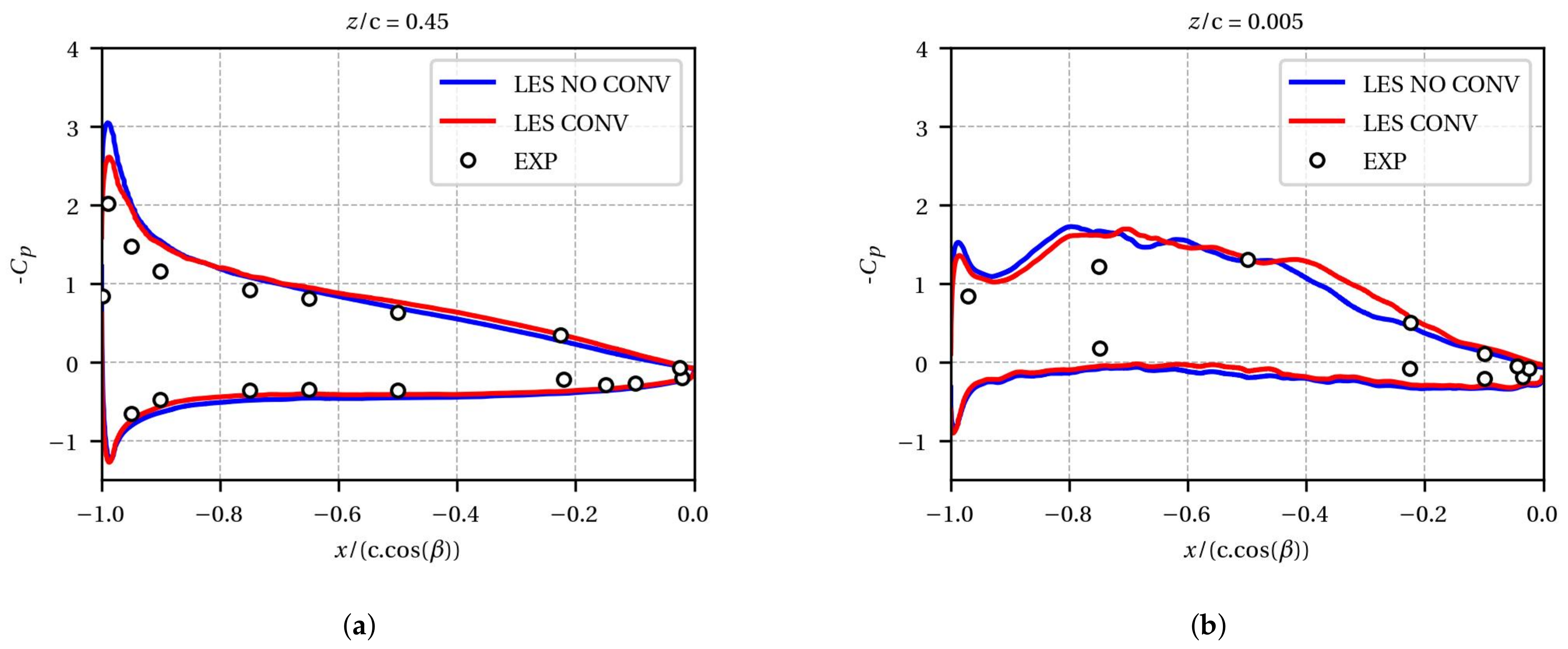
Using the previous algorithm at different spatial positions in the streamwise direction on $yOz$ planes allowed us to identify the vortex centre. The resulting trajectory projected on planes $xOy$ (Figure 8a) and $xOz$ (Figure 8b) is displayed in Figure 8 for the experiment and each LES. The airfoil is in grey. We observed that, if the correct inflow conditions were taken into account, as in the LES CONV, the experimental trajectory was well retrieved.

As explained by Storer et al. [30], the vortices at tip have an influence on the pressure on the airfoil surface. The modification of the trajectory of the tip leakage vortex observed in Figure 8 explains the difference on the pressure coefficient in Figure 6b. With the convergent, the tip leakage vortex is closer to the airfoil, as shown in Figure 8a. Therefore, the pressure on the airfoil surface is lower compared to the case without the convergent.

6. Tip Leakage Vortex Convection

In the previous section, the mean trajectory of the tip leakage vortex was improved in the LES with the convergent (Figure 8). However, the longitudinal velocity acceleration of the tip leakage vortex, that is to say the convection of the vortex, remains an issue (Figure 7).

To improve the prediction of the LES, a mesh adaptation based on the dissipation of the kinetic energy was performed. Following the approach sets up by Daviller et al. [31], a static h-refinement strategy was used to refine precisely the tip leakage vortex region. From the previous LES CONV simulation, the time-average dissipation field $\overline{\tilde{\mathsf{\Phi }}}$ is used to build a metric. The quantity of interest $\overline{\tilde{\mathsf{\Phi }}}$ is defined as:

$$\overline{\tilde{\mathsf{\Phi }}}=\overline{\left(\mu +{\mu }_t\right){\left(\frac{\partial {\tilde{u}}_i}{\partial x_j}+\frac{\partial {\tilde{u}}_j}{\partial x_i}\right)}^2}$$

(3)

with $\mu$ as the kinematic viscosity and ${\mu }_t$ as the local turbulent viscosity computed by the LES subgrid scale model. The operators $\widetilde{.}$ and $\overline{.}$ represent the LES filtered variables and the time-average, respectively. A normalization is first performed with the minimum and maximum values of $\overline{\tilde{\mathsf{\Phi }}}$:

$${\mathsf{\Phi }}^{*}={\left[1-\left({\displaystyle \frac{\overline{\tilde{\mathsf{\Phi }}}-{\overline{\tilde{\mathsf{\Phi }}}}_{\min }}{{\overline{\tilde{\mathsf{\Phi }}}}_{\max }-{\overline{\tilde{\mathsf{\Phi }}}}_{\min }}}\right)\right]}^{\alpha }$$

(4)

Then, the metric range is defined using the $ϵ$ parameter:

$$\mathrm{metric}={\mathsf{\Phi }}^{*}(1-ϵ)+ϵ$$

(5)

Using the pyhip [17] tool, 38 × 10${}^6$ tetrahedrons are added to the initial mesh, and the minimal edge size is divided by a factor of 1.12. The magnification factor is set to $\alpha$ = 100, and the minimum of the metric field to $ϵ$ = 0.7. The spatial extension of the adaptation is limited to $z_{max}$/c = 0.5 spanwise and to $x_{max}$/c = 1.25 streamwise.

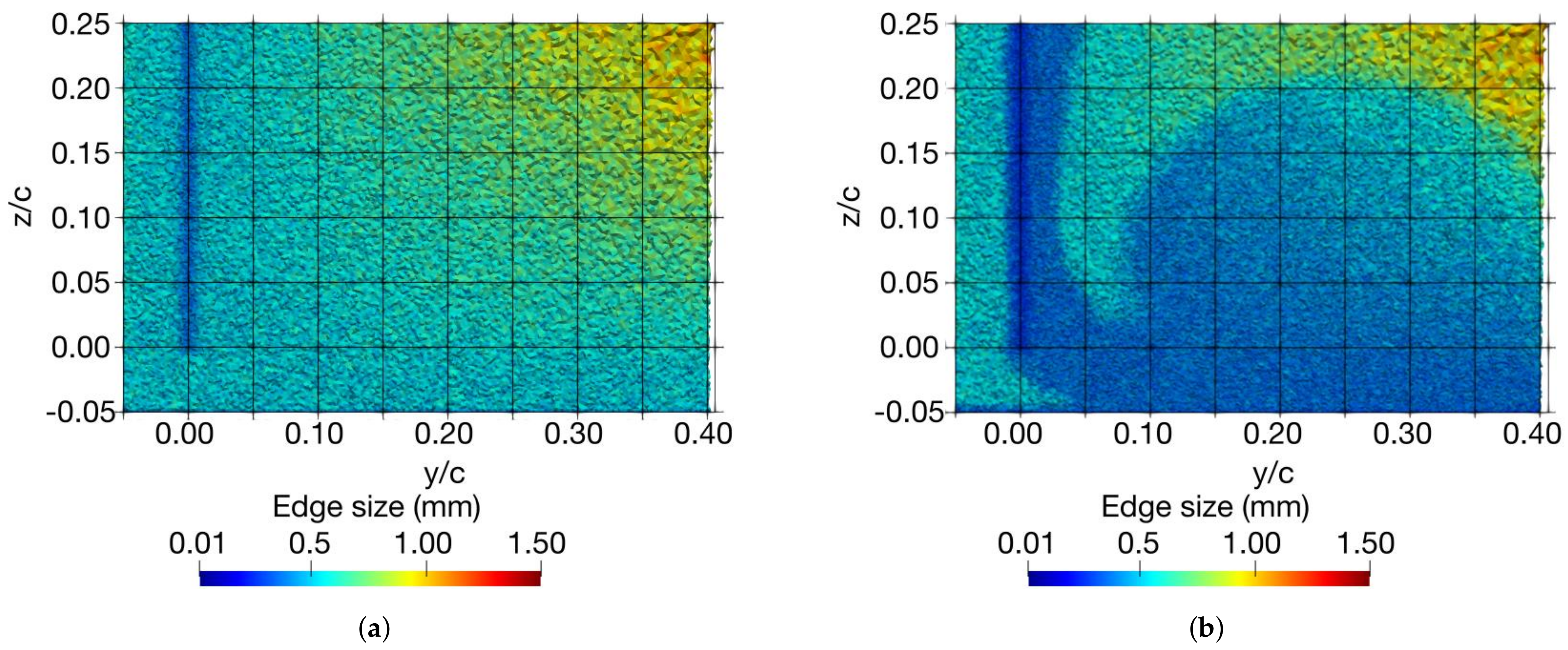
The adapted mesh at z/c = 0.1 is shown in Figure 9. The mesh was refined in the zones of interest, that is to say the tip leakage vortex, the wake, and around the airfoil surface. For the same simulated time, the computational cost was increased by 25%. The edge size of the mesh before and after adaptation at the airfoil trailing edge is, respectively, presented in Figure 10a,b.

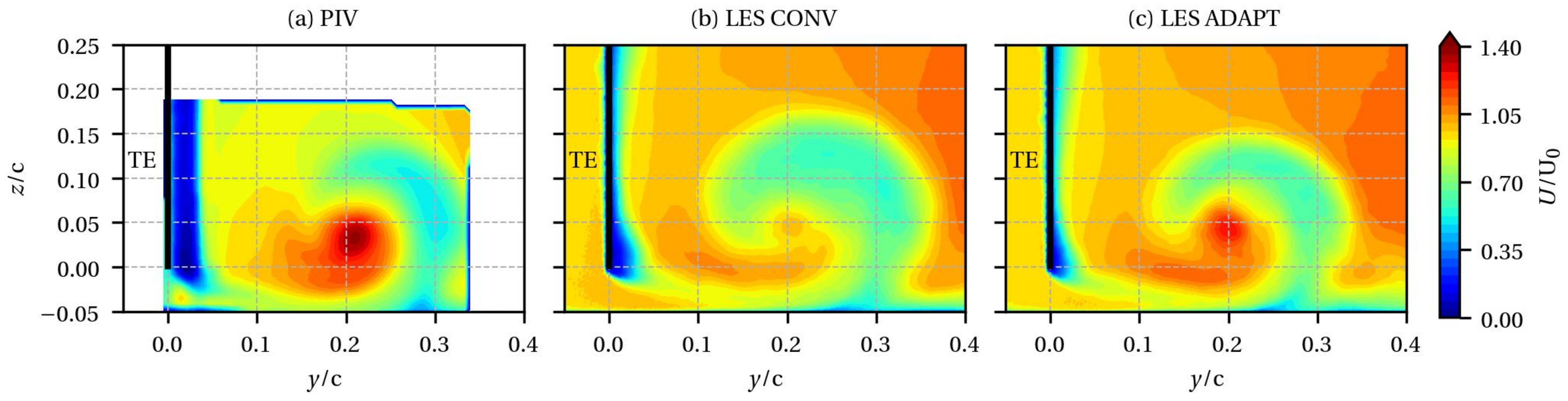
Figure 11 compares the mean axial velocity U between PIV, LES CONV, and LES ADAPT of the tip leakage vortex at the airfoil trailing edge (x/c = 0.01). With the proper mesh refinement, LES ADAPT is able to better retrieve the topology measured by the PIV. Indeed, the two velocity regions and even the position of the maximum of U are captured with less than $15\%$ of the error as PIV.

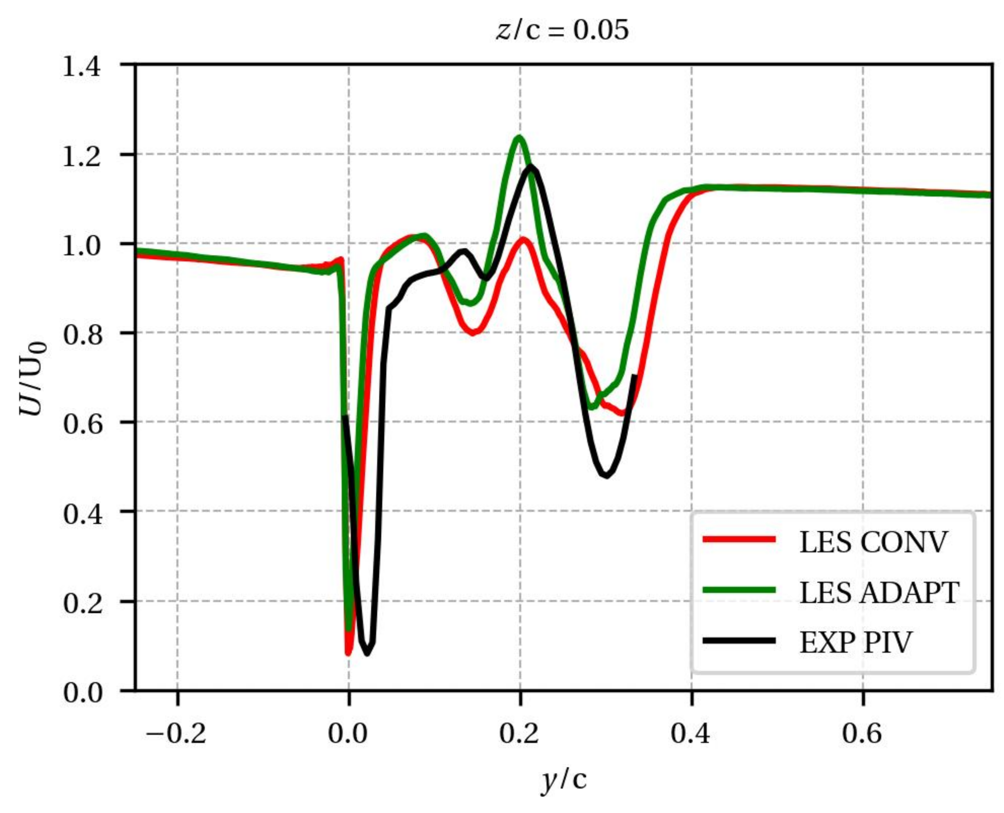
To deepen the analysis, 1D velocity profiles are plotted at z/c = 0.05 in Figure 12. Using the mesh adaptation, the predicted velocity profile is clearly improved. Indeed, whereas the deficit of velocity caused by the airfoil wake is retrieved by both LES around y/c = 0 with the correct amplitude, some discrepancies are observed in the tip leakage vortex zone, which extends from y/c = 0.17 to 0.35. Indeed, the LES with mesh adaptation in green is able to recover the amplitude of the maximum U at y/c = 0.2. Mesh adaptation allows to recover the complex structure of the tip leakage vortex and especially the acceleration of the longitudinal velocity component.

7. Spectral Signature of the Tip Leakage Flow

Regarding the high Reynolds number that characterises the flow in a real turbomachinery configuration, a wall law is required for the computational cost issue. Therefore, the capability of the wall law to predict the aerodynamics and acoustics of the tip leakage flow of the isolated airfoil is studied in this section. The wall-modelled LES performed in this paper is compared to two previous wall-resolved LES from Boudet et al. [9] and Koch et al. [10]. These two LES are achieved at an angle of attack of 15${}^{\circ }$, whereas the current LES is at 16.5${}^{\circ }$. Figure 6 shows that the wall law is able to reproduce the mean pressure distribution on the airfoil surface, especially in the tip region.

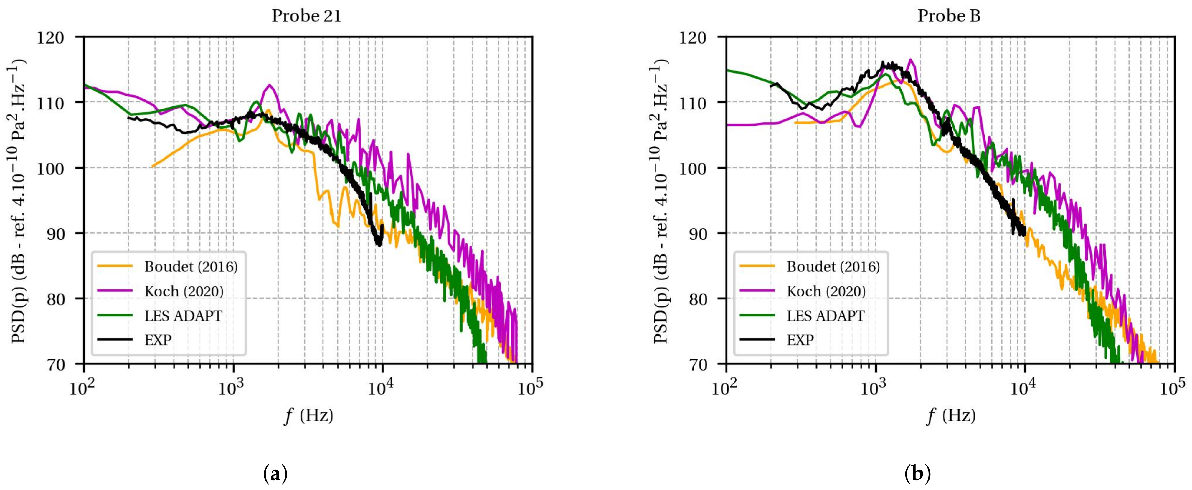
Figure 13 presents the PSD of the wall pressure fluctuations on the airfoil surface. For clarity, only results from LES ADAPT are shown. Two positions at 77.5% of chord were considered. Probe 21 (Figure 13a) is located on the airfoil suction side, 1.5-mm away from the tip, whereas probe B (Figure 13b) is on the airfoil tip, on the camber line. Since wall pressure spectra of the LES from Koch et al. are not available at 77.5%, the spectra at 75% are used in Figure 13. The three LES are compared to the measurements extracted from Jacob et al. [5]. The experimental cut-off frequency was 22 kHz; however, data were only available until 10 kHz.

For probe 21, the LES exhibits a good agreement with the experiment regarding both shape and level. The spectrum is even in better agreement than the two wall-resolved cases. The LES from Koch et al. (magenta) that was also performed with AVBP exhibits the same shape than the current LES with a shift in frequency.

On probe B, the hump around 1.3 kHz characterises the pressure fluctuations induced by the detachment of the tip leakage flow on the airfoil pressure side-tip corner. A broadband hump is observed instead of a tonal peak because of the intermittency of the phenomenon [32]. The LES is able to well retrieve the hump at 1.3 kHz. For frequencies higher than 6 kHz, a slight overprediction is observed from the experiment. The LES from Koch et al. is again showing the same trend. The ZLES from Boudet et al. remarkably predicted the wall pressure fluctuations even at high frequencies. Figure 13 shows the capacity of the wall law to predict the wall pressure fluctuations on the airfoil surface in the tip region.

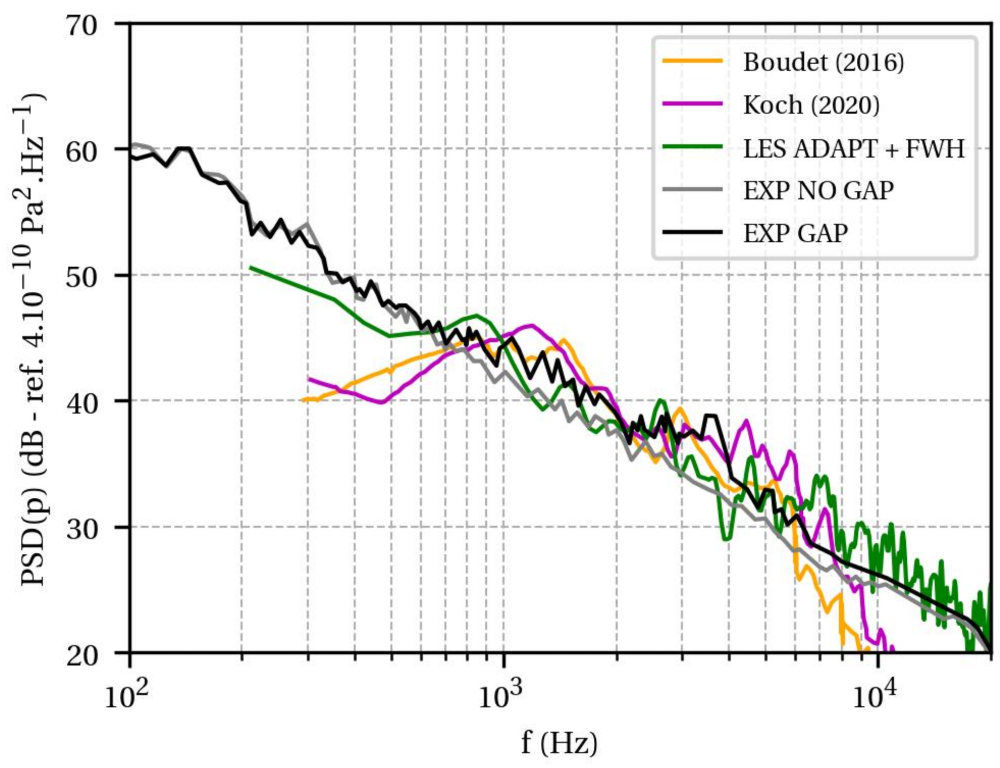
Figure 14 presents the PSD of the acoustic pressure in the far-field. The microphone was placed 2-m away from the airfoil suction side, forming an angle of 90${}^{\circ }$ with the airfoil chord. The acoustic propagation in the far-field was ensured using the solid Ffowcs–Williams and Hawkings’ analogy (FWH). This means that only the dipole sources are taken into account to estimate the sound; the aforementioned quadrupoles associated with the tip-gap jet are ignored. The python library antares [18] is used following the advanced time formulation of Casalino [33].

The microphone recorded the noise emitted by the airfoil in no-gap (grey) and 10-mm-gap (black) configurations. It allowed us to identify a frequency range of the tip clearance noise from 0.7 to 7 kHz. The wall-resolved LES in orange and magenta are able to retrieve the noise level in this range. The wall-modelled LES in green is able to predict the noise level on an even wider range of frequencies. Whereas the acoustic spectra from the two wall-resolved LES drop for frequencies higher than 7 kHz, the LES presented in this paper manages to predict the proper noise level.

It may be explained by the size of the LES domain. Indeed, Boudet et al. performed a ZLES with a LES zone reduced to the tip region and Koch et al. achieved a LES on a modified geometry with a reduced span. In both cases, the pressure fluctuations on the airfoil surface are not computed over the full span. This comparison demonstrates also the capacity of the wall law to model the tip leakage flow for the purpose of acoustic prediction.

8. Conclusions

With the aim of improving existing prediction models or to model new noise sources features of the tip clearance noise, a LES of an isolated airfoil with a gap was performed. Two computational domains with the same experimental set-up were considered, including modelling the inflow conditions. We observed that the LES with a modelling of the inflow conditions (i.e., without the convergent of the open-jet wind-tunnel facility) allows to obtain correct results in terms of airfoil loading and mean tip leakage vortex. However, some deviations were observed when compared to the measurements. In particular, the mean axial velocity of the tip leakage vortex was underestimated, and its mean trajectory was farther away from the airfoil. On the other hand, taking into account the full experimental set-up in the computational domain allowed us to correct these differences and better match the experiment. This improvement is explained by a more realistic development of the jet, which has a non-negligible interaction with the flow around the airfoil.

Moreover, we demonstrated that the use of a mesh adaptation was necessary in order to recover the complex structure of the tip leakage vortex and especially the acceleration of the longitudinal velocity component. Finally, the present wall-modelled LES methodology allowed us to accurately predict the wall pressure fluctuations on the airfoil surface and the acoustic spectrum in the far-field. In particular, the frequency range of the tip clearance noise was correctly captured.

Resorting to the LES is essential for the intended future acoustic applications, such as Ultra-High Bypass Ratio turbofan engine, the details of which are beyond the scope of the present paper. Indeed, explicit wall-pressure statistics requiring the simulation of the turbulence are generally used as input data in the sound prediction models. The wall-modelled LES strategy developed in this paper was designed to address this issue on more realistic rotating configurations.