Near-Wall Flow in Turbomachinery Cascades—Results of a German Collaborative Project

Abstract

This article provides a summarizing account of the results obtained in the current collaborative work of four research institutes concerning near-wall flow in turbomachinery. Specific questions regarding the influences of boundary layer development on blades and endwalls as well as loss mechanisms due to secondary flow are investigated. These address skewness, periodical distortion, wake interaction and heat transfer, among others. Several test rigs with modifiable configurations are used for the experimental investigations including an axial low speed compressor, an axial high-speed wind tunnel, and an axial low-speed turbine. Approved stationary and time resolving measurements techniques are applied in combination with custom hot-film sensor-arrays. The experiments are complemented by URANS simulations, and one group focusses on turbulence-resolving simulations to elucidate the specific impact of rotation. Juxtaposing and interlacing their results the four groups provide a broad picture of the underlying phenomena, ranging from compressors to turbines, from isothermal to non-adiabatic, and from incompressible to compressible flows.

1. Introduction

Present goals in the development of turbomachines for flight propulsion are oriented towards a further increase of pressure ratio and efficiency with a simultaneous reduction of the number of blades and stages of compressor and turbine [1]. For stationary gas turbines used to generate electric power, challenging demands on flexibility and operation under partial load result from the volatile availability of renewable energies [2]. These requirements on both types of systems lead to high aerodynamic loads on the blade rows and to an increase in losses due to secondary flows [3]. The latter occur mainly in regions close to sidewalls and have been the focus of scientific investigations for many years [4,5,6,7,8,9,10]. Still, however, understanding is incomplete but is required for increasing efficiency in order to meet economic and ecologic concerns.

While in current design processes the flow is mostly considered in its temporal average [11], the real flow in axial compressors and turbines is strongly unsteady, with turbulence and periodic contributions resulting from the aerodynamic interaction of the blade rows moving relative to each other [12,13,14,15]. It exhibits high complexity due to the inner and outer sidewalls and the effects generated by rotation. In fact, the near-wall flow is characterized by the wall boundary layer, blade boundary layers and the interaction of several secondary flow phenomena, such as radial gap vortex, horseshoe vortex and channel vortices, all of them being periodically unsteady in a flow field which is partly transitional and turbulent on top [16]. The cited effects occur in both, axial compressors as well as axial turbines, but differ considerably according to design features and aerodynamic blade or stage load, so that the different secondary flow phenomena have different characteristics. The intensity of the aerodynamic interaction between the blade rows qualitatively and quantitatively depends on a number of geometric and aerodynamic parameters, such as axial gap width, wake width, velocity deficit of the wake, Strouhal number, flow coefficient, etc. In numerous studies these effects have been investigated with linear cascades [17,18], and disregard of heat transfer in the case of turbines. On the opposite side, there are many studies on machines of realistic or close-to realistic complexity, with measurements usually complicated by practical aspects [19,20].

On this background four groups at three German universities have joined forces in a government-funded collaborative project aiming at the detailed investigation of the flow in the near-wall area of turbomachinery. In particular, the joined effort is dedicated to fill the gap between the two antipodes, linear isothermal cascade and complex machine with heat transfer. On the one hand, it addresses aspects of heat transfer at the sidewall during transient inflow, which have not been investigated in linear cascades so far. On the other hand, the connection between stationary linear and rotating ring cascades is investigated. The relevant aspects are the fanned blades in the ring cascade, the radial pressure gradient, the Coriolis forces and the jumps in the circumferential speed between rotor and stator generating strongly twisted sidewall boundary layers at the entry into the blade rows. The overarching goal is to investigate to which extent studies in linear cascades can provide information about the near-wall flows in the machine and how, if necessary, the data from linear cascades must be interpreted to obtain such information. This gradual increase in complexity allows to decompose the respective influences, which in the machine can only be considered as a whole, interacting with each other. To the knowledge of the authors, detailed investigations of this kind have not been available, so far.

The present paper was conceived to provide the community with a timely, condensed synopsis over the recent results achieved in this collaboration, highlighting the larger picture and, if necessary, referring to separate publications for details and side studies. To this end, the paper is structured in line with the project structure featuring four sub-projects A to D.

Sub-project A deals with skewness and periodic distortion of the sidewall boundary layer in an axial compressor cascade. Experimental investigations inside a low speed axial research compressor are performed with several configurations including rotating and fixed hub walls. Numerical studies using a URANS-code complement the experimental findings. Sub-project B employs highly accurate turbulence-resolving simulations, DNS and LES, to perform well-controlled numerical experiments based on a compressor rotor profile under the same or similar conditions as investigated experimentally in sub-project A. These investigations focus on the stepwise increase in complexity between the linear grid and the full rotating grid, addressing the impact of fanned geometry compared to linear geometry, relative motion of the sidewall, Coriolis forces, etc. An issue not discussed in the present paper is the work performed on improving the simulation methodology. While the first two sub-projects are concerned with compressor profiles sub-project C and D are oriented towards turbines. Sub-project C is conducting experimental investigations of a T106 low pressure turbine profile in a high-speed cascade wind tunnel and complements these with URANS simulations. A major focus is put on unsteady inflow conditions which impact both the inlet endwall boundary layer and the blade loading. These issues are important to clarify because of their particular influence on the heat transfer at the sidewalls. Sub-project D employs a specifically modified T106 profile suitable for the low speed turbine configuration on site. Experimental and numerical studies with wake generators are conducted to study the unsteady behavior of the boundary layers developing on the low pressure turbine stator blades as well as their effect on the secondary flow patterns under the influence of unperturbed and periodically perturbed inflow. For this purpose, high-resolution time resolving measurement techniques including hot-film probes are used.

The long-term goal of this research is to enhance the physical understanding of the transient near-wall flow effects for compressor and turbine, thus providing action points to reduce the secondary losses resulting from the aerodynamic interactions in the near-wall flow below the current state of the art, so as to improve upon present efficiencies and environmental impact.

2. Sub-Project A—Periodically Transient Near-Wall Flow within Rotating Compressor Cascades

2.1. Scope of Sub-Project A

Within sub-project A experimental investigations on different setups of a low speed research compressor are performed to achieve steps of abstraction between a linear cascade and an axial compressor. This allows for a separate analysis of different forces and effects corresponding to the rotating system, where the main considered features are the Coriolis- and centrifugal forces, the flow channel curvature, the incoming boundary layer (BL) and its skewness as well as the relative motion (RM) between the blade tip and its corresponding endwall. Furthermore, the influence of an incoming periodic distortion on the development of the tip leakage vortex (TLV) in a compressor rotor, as well as on the global parameters of flow turning, losses and total pressure rise is investigated with varying tip clearances.

The presented results give an overview of the findings from recent and current work. Thereby focusing on the effect of varying wall motion in the vicinity of a stator row and the periodic distorted inflow to a rotor row on the secondary flow in either passage. The former allows to examine the influence of a skewed inflow boundary layer, a relative motion between the stator vane tips, and the underlying hub endwall or the combination of these two on the tip leakage vortex originating from the stator vanes with hub gap.

2.2. Experimental Setup

2.2.1. Test Facility

The investigations are conducted using the Low Speed Research Compressor (LSRC) operated by the Chair of Turbomachinery and Flight Propulsion at the Technische Universität Dresden. The 4.5 stages, including an inlet guide vane (IGV) and four repeating stages, of this axial compressor are built vertically with a downward facing air flow, see Figure 1. The studied blading is derived from a middle stage of a high pressure jet engine compressor and the main characteristics are given in

Table 1. Reference setup specifications of the LSRC.

Test Rig		Operating Point
Shroud diameter	1500 mm	Rotational speed at DP	1000 rpm
Hub to tip ratio	0.84	Mass flow $\dot{\mathrm{m}}$ at DP	25.35 kg/s
Rotor R1		Stator S1
No. of blades	63	No. of vanes	83
Chord length	110 mm	Chord length	89 mm
Solidity, MS	1.597	Solidity, MS	1.709
Reynolds number at entry, MS	$6.5\cdot {10}^5$	Reynolds number at entry, MS	$3.7\cdot {10}^5$
Mach number at entry, MS	0.25	Mach number at entry, MS	0.18
Flow coefficient φ, MS 1	0.651	Diffusion factor, MS	0.37
Loading coefficient $\left(\frac{\Delta h_t}{u^2}\right)$, MS 1	0.489

¹: at 10% higher mass flow than DP due to the discarded IGV in test setup (b).

. For further information on the LSRC please refer to Boos et al. [21] and Künzelmann et al. [22].

To evaluate the effects of varying motion of the wall and incoming periodic distortions two major setups are observed, shown in Figure 1. For the first configuration (a) the object of investigations is the stator of stage 1 (hereinafter referred to as stator 1). An adjusted IGV with 83 vanes produces the proper inflow conditions and allows direct periodicity for the later numerical computations. The blades of stage 1 are dismounted from the rotor disk, which can be set to the design rotational speed inducing a skew of the sidewall boundary layer. Replacing the rotor disk with a stationary band consisting of 12 circumferentially divided segments allows investigations with stationary sidewalls and thus suppressed inlet BL skew to stator 1 (S1). In addition to the change of the hub endwall upstream of S1, the shroud ring of the stator can be replaced by a rotating hub ring allowing a relative motion between hub and stator vanes. For the latter case, the stationary ring over the rotor hub cannot be used due to constructive restrictions, thus three different cases can be investigated experimentally, see

Table 2. Configurations of varying wall speed for test setup (a).

Configuration	Rotor R1 Hub Wall	Stator S1 Hub Wall
Un-skewed, w/o RM	Stationary	Stationary
Skewed, w/o RM	Rotating	Stationary
Skewed, with RM	Rotating	Rotating

.

Comparing these configurations allows to evaluate the influence of a skewed inflow BL, which is associated with the movement of the hub wall at the rotor of stage 1 (hereinafter referred to as rotor 1), and the relative motion between the vane tip and the adjacent wall, which is induced by not using shrouded stator vanes. These investigations are carried out with different stator hub clearances. For stationary hub endwall the no clearance (s/C = 0.0%) and three gap sizes with clearance heights (s) normalized by chord length (C) of s/C = 2.0%, s/C = 5.4% and s/C = 6.7% are realized, while a few non-clearance vanes supported the shroud ring. With rotating hub endwall only non-zero clearances are tested. Leakage flow through axial gaps in the hub is considered negligible due to a minor pressure difference between the rotor drum and the flow channel, as well as small gaps of under 1 mm. Downstream of S1 all blades and vanes are dismounted except of stage 4, which is used to drive the flow.

For test setup (b) only rotor 1 (R1) is bladed. Two tip gap sizes of s/C = 1.36% and s/C = 4.55% are observed which allows to evaluate the influence of incoming periodic distortions in dependence upon the tip clearance size. Either installing or discarding a wake generator (WG) produces the distorted, from here on unsteady, or the not distorted, from here on steady, inflow. The WG consists of 83 circumferentially arranged circular bars with a diameter of D_b = 2 mm. They are mounted 65.6% C upstream of the R1 leading edge (LE). This approach allows the analysis of the effect of an isolated wake disregarding the complex secondary flow field of a stator row. Furthermore, it enables a more direct comparison to linear cascade investigations where an analog setup was examined, cf. Krug et al. [23]. Due to the discarded IGV, the mass-flow rate is adjusted to ensure the same rotor entry incidences as for the design point (DP) resulting in an adjusted design point at 10% higher mass-flow. All rotor data shown here correspond to this operating point. As this paper gives a short overview of the work done, only the nominal tip clearance cases, s/C = 2.0% for the stator and s/C = 1.36% for the rotor, will be presented here.

2.2.2. Measurement Techniques

The flow field can be captured in several measuring planes (MP) perpendicular to the machine axis, see Figure 1, using various probes. For the presented results only two MP are of interest. The first one is MP4 which is located 26.8% C_ax,R1 downstream of the trailing edge (TE) of R1, and at once located 16.3% C_ax,S1 upstream of the LE of S1. The second one, MP5, is positioned 21% C_ax,S1 downstream of the TE of S1. At both positions the measuring probes can be traversed radially and rotated around their axis. All stator rows are rotated simultaneously around the machine axis to alter the relative position between probe and stator vanes in pitchwise direction. Five-Hole-Probes (FHP) with spherical heads of a diameter of 2 mm are used to capture the steady flow field. Balancing the pressures in the two lateral holes via probe rotation allowed to measure the magnitude and direction of the velocity in absolute frame of reference with an accuracy of $\Delta \mathrm{v}=\pm 0.3 \mathrm{m}/\mathrm{s}$ and $\Delta \mathsf{\alpha }=\pm 0.26°$, respectively. The unsteady flow field is acquired using a fast measuring pressure probe (FMP), designed and manufactured at the chair of Turbomachinery and Flight Propulsion in Dresden. This one-hole-probe is equipped with a piezoresistive pressure sensor, see also Lange et al. [24]. Measurements with the FMP are performed at three different angles ($\Delta \mathsf{\alpha }=30°$) virtually creating a three-hole-probe. In the presented results the unsteady flow field data is analyzed by either looking at the time or ensemble average.

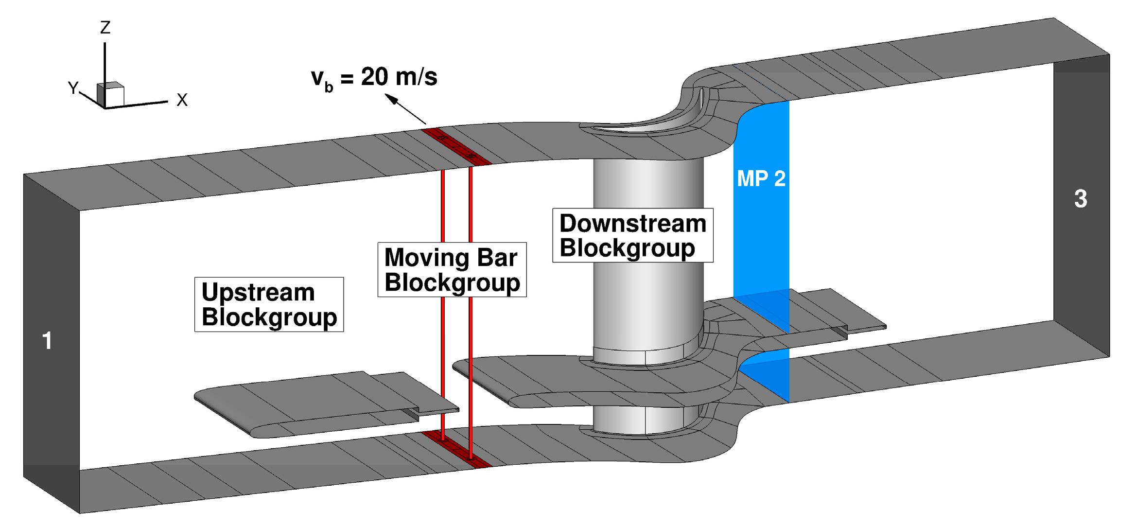
2.3. Numerical Setup

The commercial flow solver FINE^TM/Turbo by NUMECA is applied to calculate the three-dimensional RANS equations for the investigated stator cases. Analog to the experiments the combination of IGV and S1 is simulated in a single passage with periodic boundary conditions. The upstream generated wake is passed-through the domain using a perfect connection interface (Full Non Matching Frozen Rotor). The Explicit Algebraic Reynolds Stress Model (EARSM) is exploited to close the system of equations, which was found to deliver the best agreement with experimental results compared with other RANS turbulence models available in the flow solver for the LSRC, see also Lange et al. [24].

The domain is discretized applying a block-structured mesh with O4H-topology around the vanes, OH-topology in the tip gap and H-topology in the remaining parts. A preceding sensitivity study ensured a minimized spatial discretization error. Herein, especially the number of cells in streamwise direction within the empty duct between IGV and S1 was found to have a noticeable effect on the sustaining of the wake, see also Busse et al. [25]. As the BL is of particular interest, it is resolved, leading to dimensionless wall distances y⁺ of around 1. In spanwise direction the average density of grid nodes in the tip gap is held constant at a ratio of 22 cells per 1% of gap size normalized by channel height (s/H). The number of cells in the remaining flow channel is adjusted analogously resulting in final meshes with $1.0\cdot {10}^7$ up to $1.5\cdot {10}^7$ grid points.

2.4. Current Investigations and Results

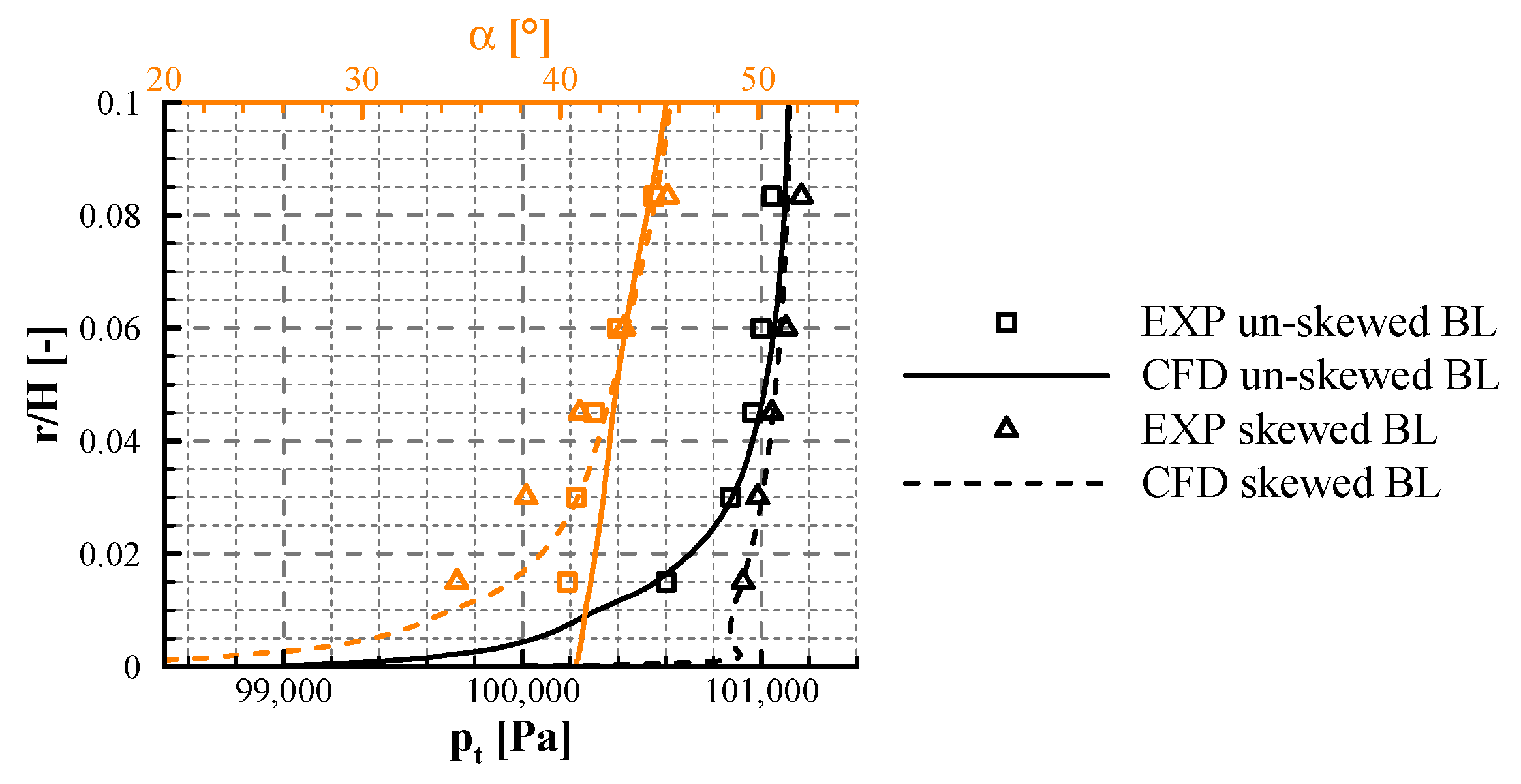
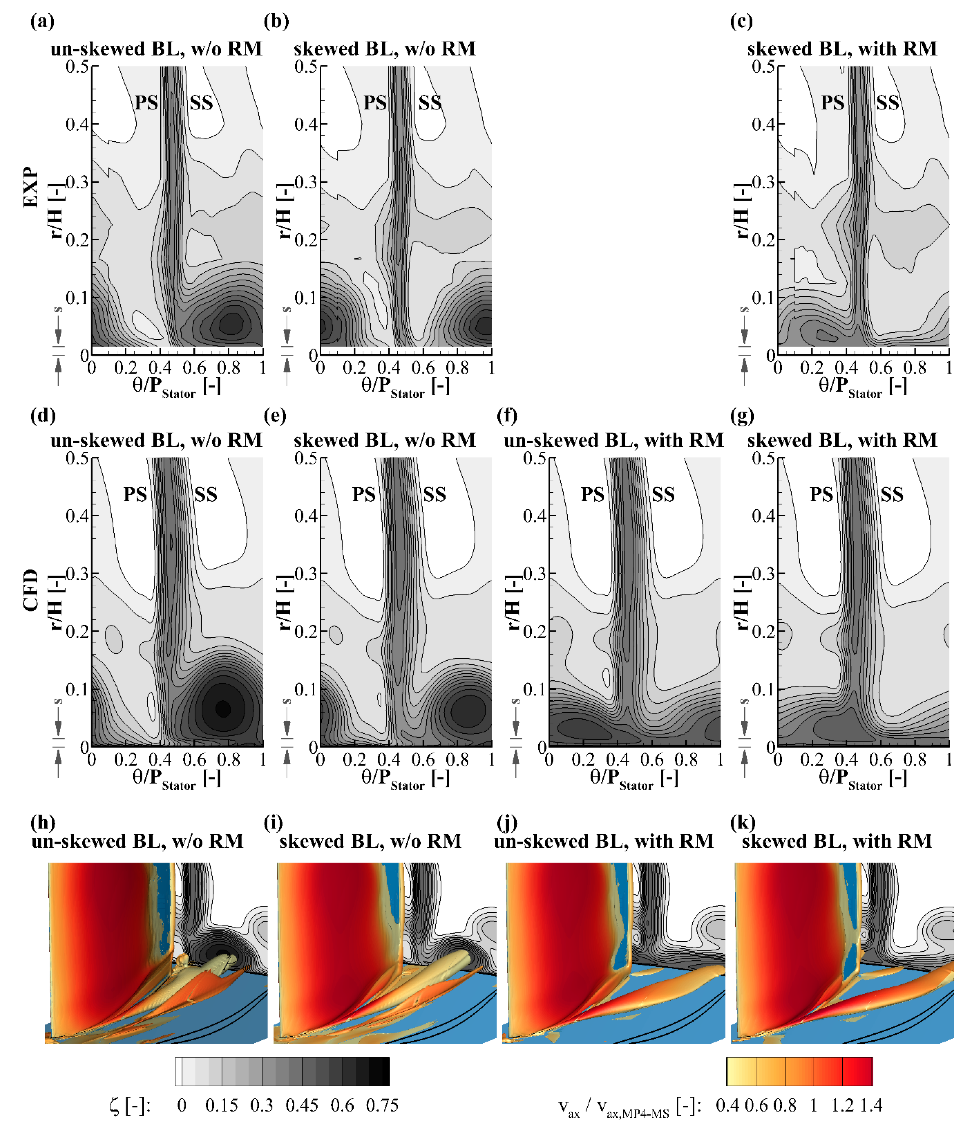
2.4.1. Influence of the Inlet Boundary Layer Skew

The influence of a skewed inlet BL is investigated by comparing the shrouded stator cases with the rotating R1 disk, inducing a skewed BL, and the cases with the stationary band, suppressing the skewness and thereby producing an un-skewed BL. The difference in inflow can be seen in Figure 2, where the pitchwise averaged radial distributions of total pressure p_t (in black) and flow angle in absolute frame of reference α (in orange) are shown for MP4. Here lines, solid for un-skewed and dashed for skewed BL, represent results from computational fluid dynamics (CFD) calculations and the symbols, square for un-skewed and delta for skewed BL, denote to the experimental data (EXP).

The skew of the incoming BL is clearly detectable by the strong drift of flow angle α towards lower values at relative channel heights (r/H) below 5% for the test configuration with rotating R1 disc, cf. Figure 2. The resulting turning of the flow corresponds to higher total pressure in this area as it induces energy into the flow. In contrary a decrease in total pressure values towards the hub can be seen for the test case with a stationary band upstream of S1 forming a typical BL. This is accompanied by a constant decline in flow angle down to the hub endwall in the depicted channel region remaining at higher values compared to the skewed BL configuration.

To analyze the secondary flow in the downstream measuring plane (MP5) the non-dimensional total pressure loss coefficient ζ is defined by

$$\mathsf{\zeta }\left(\overrightarrow{\mathrm{x}}\right)=\frac{\overline{{\mathrm{p}}_{\mathrm{t},\mathrm{ref}}}-{\mathrm{p}}_{\mathrm{t}}\left(\overrightarrow{\mathrm{x}}\right)}{\overline{{\mathrm{p}}_{\mathrm{dyn},\mathrm{ref}}}}.$$

(1)

Here the pitchwise averaged total and dynamic pressure in the upstream plane (MP4) at midspan (MS), $\overline{{\mathrm{p}}_{\mathrm{t},\mathrm{MP}4,\mathrm{MS}}}$ and $\overline{{\mathrm{p}}_{\mathrm{dyn},\mathrm{MP}4,\mathrm{MS}}}$, are used as reference. For the nominal clearance case of s/C = 2.0% the ζ contours in MP5 are shown for skewed and un-skewed inflow BL without relative motion (RM) of the hub endwall in Figure 3a,b. A deviation in position of the TLV, represented by the circular areas of high ζ, is apparent with an approximated shift of the core of 0.15 θ/P_Stator in pitchwise direction, where θ/P_Stator corresponds to the circumferential distance normalized by S1 pitch. In a compressor cascade a skewed inlet BL reduces the cross passage flow in the vicinity of the hub as its direction of influence directly opposes the pressure gradient from pressure side (PS) to suction side (SS) of two adjacent vanes. This weakens the passage vortex and was observed for a linear compressor cascade by Moore and Richardson [26]. In the current work these findings were confirmed for the axial machine in a non-clearance case for S1, cf. Koppe et al. [27].

The reduced strength of the passage vortex implicitly decreases its influence on the TLV, as these two vortices have opposing directions of rotation. Furthermore, the drift to smaller values of flow angle in absolute frame of reference (α) in the vicinity of the hub endwall leads to higher loaded profiles at vane tip, favoring a detachment of the flow from the SS. The result can be seen in Figure 3b for the skewed BL case, where the TLV detaches from the stator vane somewhere along the chord and moves pitchwise into the passage. The trajectory of the TLV follows the SS of the vane for an un-skewed incoming BL and thereby a connected area of high non-dimensional total pressure loss coefficient of the TLV and the vane wake can be seen, cf. Figure 3a. A decrease in effect of the boundary layer skewness on the TLV is observed with increasing tip clearance height, not shown here, cf. [27]. This is expected as the area of influence of this phenomenon is restricted close to the endwall.

Radial profiles of flow angle in the absolute frame of reference are plotted for S1 test configurations with varying hub endwall motion in Figure 4. At relative channel heights between 5 and 25% higher flow angle values representing higher turning over the stator row are detectable for the skewed BL case without relative motion between vane tip and underlying hub endwall. Below 5% r/H the relation reverses and lower values of flow angle can be seen for the skewed BL setup. This coincides with the reduction in cross passage flow in the vicinity of the hub for an incoming skewed BL.

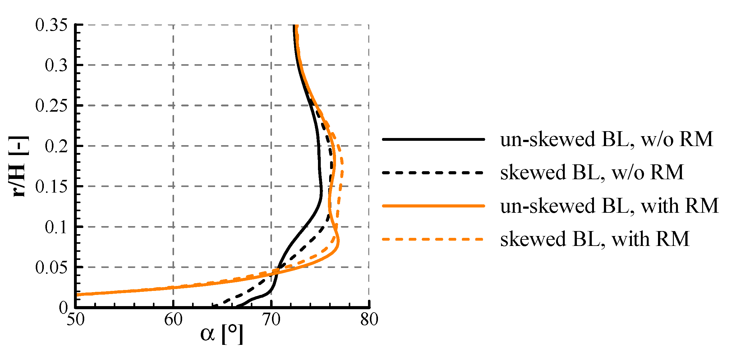
2.4.2. Influence of Relative Motion between Vane Tip and Corresponding Endwall

Due to constructive restrictions it is not possible to experimentally evaluate the isolated effect of the relative motion between the vane tips and the underlying hub endwall on the TLV, see also Section 2.2.1. For this purpose, the numerical method is conducted. This is suitable as the results from the CFD show good agreement with the experiments for the other three cases, see Figure 3. An overprediction of the losses associated with the TLV is apparent for the numerical results, which is assumed to be due to the computational model not being able to correctly capture the turbulent structures of the TLV. Nevertheless, size and position of the TLV agree for the different endwall motion cases between numerical and experimental data to a sufficient extent rendering the following discussion valid, see also Koppe et al. [27].

To evaluate the influence of a relative motion between the vane tip and its corresponding endwall on the TLV the two cases, one with stationary and one with rotating hub at S1, without an incoming BL skew are observed, see Figure 3d,f. For the combination of un-skewed BL without relative motion the TLV stays attached to the SS of the vane, indicated by the big area of high non-dimensional total pressure loss coefficient located adjoining to the vane wake region of high ζ, see Figure 3d. Introducing a relative motion of the hub endwall a reduction in spanwise size of the affected passage area as well as a drift of the vortex core towards the adjacent vane PS is apparent, see Figure 3f.

The flow in the vicinity of the hub endwall features two opposing secondary flows when the stationary shroud ring is installed. The first resulting from the pressure gradient between the pressure and suction side of two adjacent vanes, the cross passage flow, and the second arising from the flow over a vane tip, the tip leakage flow, which rolls up into the TLV and continues further downstream. The cross passage flow aids to the tendency of the TLV to follow the SS contour of the vane where it emerged. The vortical structures within the lower half of the stator passage are visualized via isosurfaces of the ${\mathsf{\lambda }}_2(\langle \overrightarrow{\mathrm{v}}\rangle )$ vortex identification criterion, cf. [28], in Figure 3h. Here an additional smaller secondary vortex is identifiable next to the TLV which is induced by the interaction of the cross passage flow and the TLV. Its rotational direction is opposing to the TLV’s and thereby adding to the prior described trend of following the SS contour. For the case with RM the cross passage flow is suppressed by the no-slip condition on the hub endwall, which also has a dragging effect on the TLV. Hence, a shift of the TLV’s trajectory in the direction of the wall movement, which is towards the adjacent vanes PS, is apparent. This dragging effect as well as a higher interaction of the TLV with the free passage flow reduces its extension in spanwise direction. The apparent decreased values of non-dimensional total pressure loss coefficient in MP5, see Figure 3f, must be put into perspective considering the insertion of energy into the boundary layer flow of the hub endwall due to its rotation. The aforementioned secondary induced vortex is not distinctly identifiable here, see Figure 3j.

Looking at the pitchwise averaged distributions of flow angle α, Figure 4, an increase in values between 5 and 25% of relative channel heights is visible for the un-skewed BL case with RM compared to the case without, as was seen for the skewed BL configuration, cf. Section 2.4.1. Here, the distributions follow a similar trend down to around 11% r/H where a sudden further increase in flow angle is detected for the setup with relative motion. Comparing to the 2D plot of non-dimensional total pressure loss, this relative channel height corresponds to the upper bound of regions with higher losses associated with the TLV, see Figure 3f. With the relative endwall motion reducing the spanwise and increasing the pitchwise expansion of the TLV, the overall influence of the vortex on the pitchwise averaged flow angle at these radial positions will increase. As the orientation of rotation of the TLV favors higher flow angles in the upper part of the vortex, the sudden increase in values is reasonable. Below the vortex core this trend will reverse adding to the extensive influence of the moving endwall resulting in the clear drift towards smaller flow angle values for the case with RM in the vicinity of the hub (r/H = 0), see Figure 4.

2.4.3. Combined Influence of Boundary Layer Skew and Relative Motion between Vane Tip and Corresponding Endwall

Setting the hub endwall for stage 1 to the design rotational speed the combined effect of a skewed inflow boundary layer and a relative motion between the vane tip and the underlying wall can be analyzed. Comparing Figure 3a,c for the experimental and Figure 3d,g for the numerical results, it becomes clear that the influence upon the trajectory of the TLV increases. Both phenomena weaken or rather eliminate the cross passage flow between the PS and SS of two adjacent stator vanes in the vicinity of the hub, which in return decreases the passage vortex in this area considerably. Consequently, the progression of the TLV is less influenced by this contra rotating secondary flow. The dragging effect arising from the no-slip condition on the hub endwall further accommodates the drift of the TLV away from its originating vane towards the adjacent PS. The numerical comparison of analog configurations within a linear compressor cascade shows similar influence on the secondary flow, see Section 3.4.4. The decrease of ζ for the case with rotating hub endwall, cf. Figure 3c,g, again, must be put in perspective as the rotation of the hub under S1 induces a flow turning and by this adding energy to the fluid. It is clear, however, that the influence of the high loss region associated with the TLV on the free passage flow is far smaller for the case with a skewed BL and RM.

2.4.4. Influence of Incoming Periodic Wakes

To evaluate the influence of incoming periodic distortions on the passage flow of rotor 1 essentially isolated wakes are produced upstream using the WG. Looking at time- and pitchwise averaged radial profiles of axial velocity normalized by the midspan value at MP4 a minor redistribution in mass flow over the blade height is apparent for the unsteady case with incoming wakes, cf. Figure 5a. Here steady state measurements of the FHP (solid lines) and time resolved data from the FMP (dashed-dotted lines) are shown. Although these differ marginally in absolute value, the trends correspond well, especially when comparing the differences between the steady and unsteady R1 cases. At spanwise positions between r/H = 0.5 and 0.72 higher axial velocity can be seen for the undisturbed rotor (black lines) for both probes. In regions below midspan down to r/H = 0.19 the steady case shows lower relative axial velocity compared to the periodically disturbed rotor (red lines). The corresponding 2D flow field at MP4, captured by the FMP, is shown in Figure 5b. Here the aforementioned redistribution is evident in a weaker SS flow separation in the lower half of the passage, which is represented by the broadened area of low non-dimensional axial velocity in the blade wake. Furthermore, minor changes in the tip region can be observed for the unsteady case where the extend of low relative axial velocity decreases in size compared to the steady inflow condition.

A closer look at the unsteady case is given in Figure 5c where four distinct relative positions between WG and R1 are shown. Here, a fluctuation of the TLV can be observed by the change in the region of low non-dimensional axial velocity throughout the four time steps. At each time step the remains of incoming bar wakes are marked with yellow dashed lines and can be identified by areas of reduced relative axial velocity. They progress from left to right with each time step. From relative position one (Δθ/P_WG = 0.00) to two (Δθ/P_WG = 0.25) a reduction in low non-dimensional axial velocity is observed in the tip region where the deterioration progresses as the bar wake approaches the rotor. After passing the rotor wake, the area of low relative axial velocity in the vicinity of the blade tip strengthens again and increases with growing distance of the WG wake, as can be seen in time steps three (Δθ/P_WG = 0.50) and four (Δθ/P_WG = 0.75).

In the lower half of the passage an effect of the WG wake on the suction side separation is observed. Here, a decrease is particularly apparent when the incoming wake is in the vicinity of the rotor wake, see time steps Δθ/P_WG = 0.25 and Δθ/P_WG = 0.50 of Figure 5c. This leads to the assumption that the incoming wake influences the transition on the blade profile, which was observed for the linear compressor cascade as well as for the axial turbine configuration, see Section 3.4.5 and Section 5.4.2 respectively. Another explanation could be radially varying pressure profiles on the rotor surface due to the change of the TLV in the tip region. Further investigations are necessary to verify these hypotheses.

2.5. Work in Progress

Further analysis of the effect of incoming wakes on the TLV of the low-speed compressor rotor with increased tip clearance is under investigation and will be compared with corresponding data from previous linear cascade tests. Additional data will be obtained through particle image velocimetry (PIV) within the blade passage and hot-film CTA measurements of the profile boundary layer development. This data will be used to validate own URANS and LES results of sub-project B. Joint analysis will deepen the physical understanding.

3. Sub-Project B—High Fidelity Numerical Investigations of the Secondary Flow in a Linear Compressor Cascade

3.1. Scope of Sub-Project B

The general approach of sub-project B in the collaborative project is to use numerical simulations with two complementary objectives. First, the physics of secondary flows in the near-wall area of a compressor cascade is investigated with the goal of identifying the role of different issues, in particular those distinguishing the situation in a linear cascade from an annular cascade, with the long-term goal to elucidate the transferability of results from linear cascade studies to annular cascades. In this perspective, specific parameters, such as the relative wall motion, are investigated concerning their effect on the dominating vortical structures inside the cascade, such as the tip leakage vortex (TLV). The second goal of sub-project B is to improve the simulation methodology in the context of LES for turbomachinery flows. This unfolds in two aspects, assessing the modelling in the endwall region and identifying specific requirements in linear and annular cascades.

Based on these objectives, results of Large Eddy Simulation (LES) of a linear compressor cascade are presented. As a validation step, the modelling introduced through LES is first assessed against highly resolved data obtained by means of Direct Numerical Simulation (DNS).

3.2. Geometry

The studied geometry was defined according to the linear cascade setup of the Chair of Turbomachinery and Flight Propulsion at TU Dresden conducting sub-project A [23]. The blade profile represents a scaled tip section of the reference built rotor of the LSRC [21,22] described in Section 2.2.1. In the current investigations the linear cascade has a chord length of $\mathrm{C}=159.6 \mathrm{mm}$, an aspect ratio of $\mathrm{H}/\mathrm{C}=1.133$, and is mounted with a stagger angle of 46.9°. The leading and trailing edge profile angles are ${\mathsf{\beta }}_{\mathrm{LE}}=60.75°$ and ${\mathsf{\beta }}_{\mathrm{TE}}=40°$, respectively. The cascade has a solidity of $\mathsf{\sigma }=\mathrm{C}/\mathrm{P}=1.55$. Furthermore, the present case features a tip gap of width $\mathrm{s}/\mathrm{C}=3\% (\mathrm{s}/\mathrm{H}=2.65\%$) between the endwall and the blade tip. The endwall is located at the bottom of the computational domain, where $\mathrm{z}=0$. A sketch of the blade profile is depicted in Figure 6.

3.3. Numerical Setup and Grid

The in-house code LESOCC2 [29] was used to solve the Navier-Stokes equations in their incompressible non-dimensional form. It features 2nd order finite volume discretization in space, and time integration is performed through a 3-step 2nd order Runge-Kutta scheme. The solver has been used previously in DNS studies of linear turbine cascades, including secondary flows, providing good results [30,31,32].

In the following mainly results of Wall-Resolving Large Eddy Simulations (WRLES) at ${\mathrm{Re}}_{\mathrm{C}}=3\cdot {10}^5$ are presented. This set-up matches the configuration of Krug et al. [23]. Inlet velocity $\left|\left|{\overrightarrow{\mathrm{v}}}_{\mathrm{ref}}\right|\right|$ and blade chord $\mathrm{C}$ were used to define the Reynolds number. For the LES, the WALE model [33] was used to model the subgrid scales. Additionally, results obtained through DNS and WRLES at ${\mathrm{Re}}_{\mathrm{C}}=1.46\cdot {10}^4$ are first discussed for validation of the method. The lower Reynolds number was chosen to obtain sound reference data by simulating the configuration described using DNS with reasonable computational resources.

In all cases the computational domain covers one period of the cascade (Figure 6) which reaches from $\mathrm{x}/\mathrm{C}=-0.437$ to $\mathrm{x}/\mathrm{C}=1.367$ and was discretized using block-structured grids. For the WRLES, grid sizes with ${\mathrm{y}}^{+}\approx 1$ at the walls were ensured, resulting in a grid of 90 MCV (million control volumes). For the DNS case at ${\mathrm{Re}}_{\mathrm{C}}=1.46\cdot {10}^4$, besides the wall grid sizes, it was ensured that the cell size, defined as the cubic root of the cell volume, is smaller than the Kolmogorov scale, which was estimated using the turbulent dissipation. This resulted in a grid of 350 MCV, with 304 cells in the spanwise direction, 84 of them within the gap region. For the analogous WRLES only the restriction on wall resolution ${\mathrm{y}}^{+}$ was kept, together with the corresponding tangential resolution requirements [34], allowing to decrease the overall number of grid points down to 60 MCV for ${\mathrm{Re}}_{\mathrm{C}}=1.46\cdot {10}^4$.

Regarding boundary conditions, an unsteady turbulent flow was imposed at the domain inlet and a convective condition was set at the outlet. The turbulent inflow conditions were generated through a precursor simulation, enforcing mean and fluctuation profiles from experiments [23], with a boundary layer thickness at the inlet of ${\mathsf{\delta }}_1/\mathrm{C}=0.222 \left({\mathsf{\delta }}_1/\mathrm{H}=0.198\right)$ and a turbulence intensity $\mathrm{TI}<1\%$ at midspan [35]. At the endwall, no-slip conditions were imposed, while at the midplane symmetry conditions were applied. The domain size in spanwise direction is large enough so that the midplane boundary conditions do not influence the secondary flow.

The simulations were run for 5 flow through times (FTT) before averaging was carried out for another 15 FTT. Here, a FTT is defined based on the axial chord length ${\mathrm{C}}_{\mathrm{x}}$ and the velocity at the inlet midplane $\left|\left|{\overrightarrow{\mathrm{v}}}_{\mathrm{ref}}\right|\right|$. Simulations with still longer time integration were performed to ensure that the time integration applied here is long enough.

3.4. Current Investigations and Results

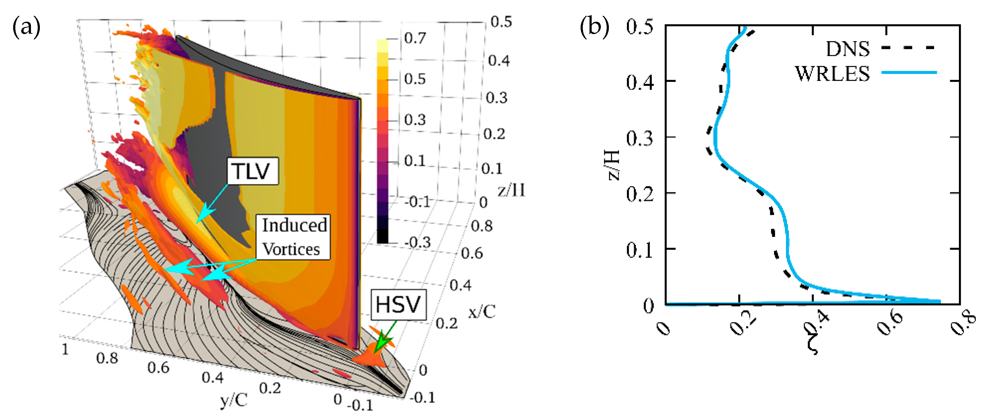
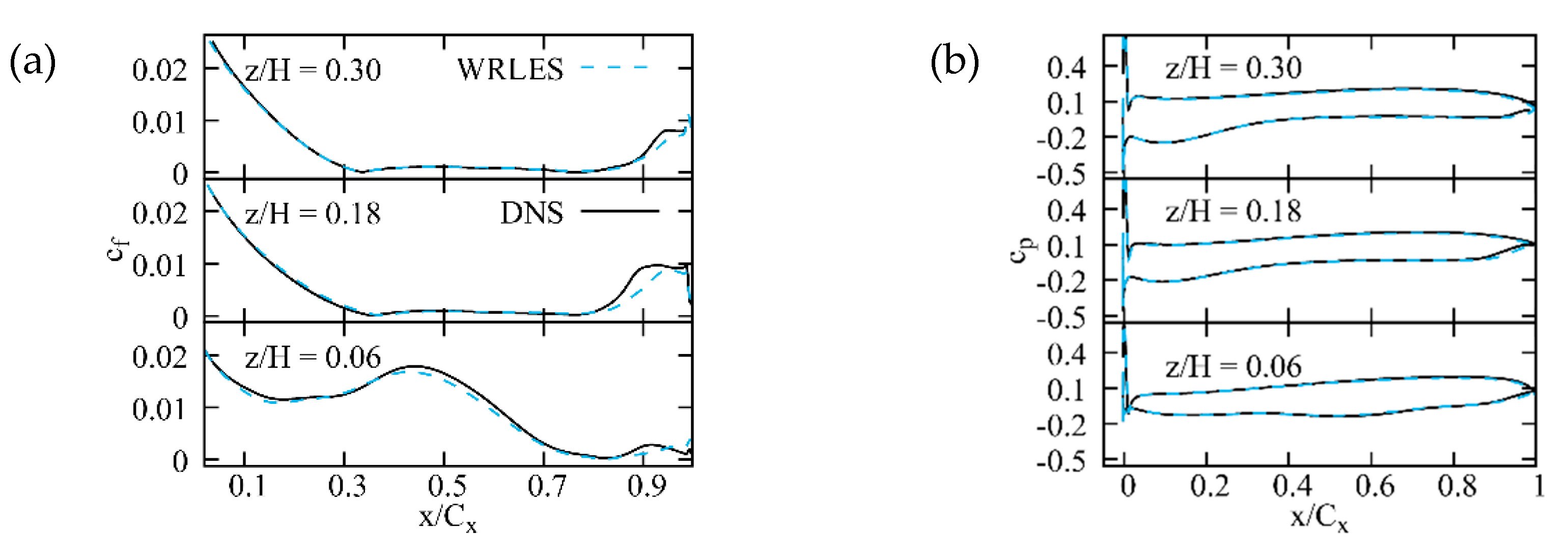
3.4.1. Validation of WRLES with Respect to DNS Data

The first step taken towards the analysis of the secondary flows in the compressor cascade is to assess the effects of the modelling approach. To this end WRLES of the compressor cascade is compared against DNS for ${\mathrm{Re}}_{\mathrm{C}}=1.46\cdot {10}^4$. As discussed in Section 3.3 the WRLES approach required only a 6th of the grid points. The overall flow structure, visualised through ${\mathsf{\lambda }}_2(\langle \overrightarrow{\mathrm{v}}\rangle )$ isosurfaces exhibits no remarkable differences (Figure 7a shows only WRLES) between both approaches.

Slight differences are related to small vortices not resolved by the LES since they are smaller than the grid size. At the outlet plane similar trends between DNS and WRLES are observed. For instance, pressure losses at the exit plane for the WRLES case, see Figure 7b, are in very good agreement with the DNS result, with slightly higher losses for the WRLES. Similarly, the pitchwise averaged exit flow angle shows a very good match. The deviations occur mainly away from the endwall. The reason for this behaviour is that near walls the WRLES grid is close to DNS resolution. Therefore, boundary layer flows around walls in the WRLES case are resolved with high fidelity. Away from the endwall differences result from a difference in the flow separation at the blade TE. This is observed, for instance, through the friction coefficient

$${\mathrm{c}}_{\mathrm{f}}={\mathsf{\tau }}_{\mathrm{w}}/\left(\mathsf{\rho }{\left|\left|{\overrightarrow{\mathrm{v}}}_{\mathrm{ref}}\right|\right|}^2/2\right)$$

(2)

at different spanwise locations, shown in Figure 8a, revealing overall very good agreement, except for $(\mathrm{x}/\mathrm{C}>0.9)$, where the WRLES predicts lower ${\mathrm{c}}_{\mathrm{f}}$ values and a later but somewhat stronger increase. Similar findings were observed in simulations of a turbine stage by Michelassi et al. [36]. These differences lead to differences in the wake, which beside the modelling uncertainty, result in the deviations presented. Nonetheless, apart from the trailing edge region the DNS data are well reproduced, with a 6-fold reduction in computational resources.

The aerodynamic blade loading is shown in Figure 8b by means of the pressure coefficient

$${\mathrm{c}}_{\mathrm{p}}=\left(\mathrm{p}\left(\overrightarrow{\mathrm{x}}\right)-{\mathrm{p}}_{\mathrm{ref}}\right)/\left(\mathsf{\rho }{\left|\left|{\overrightarrow{\mathrm{v}}}_{\mathrm{ref}}\right|\right|}^2/2\right)$$

(3)

at different spanwise positions on the blade. Here, the reference is reproduced extremely well.

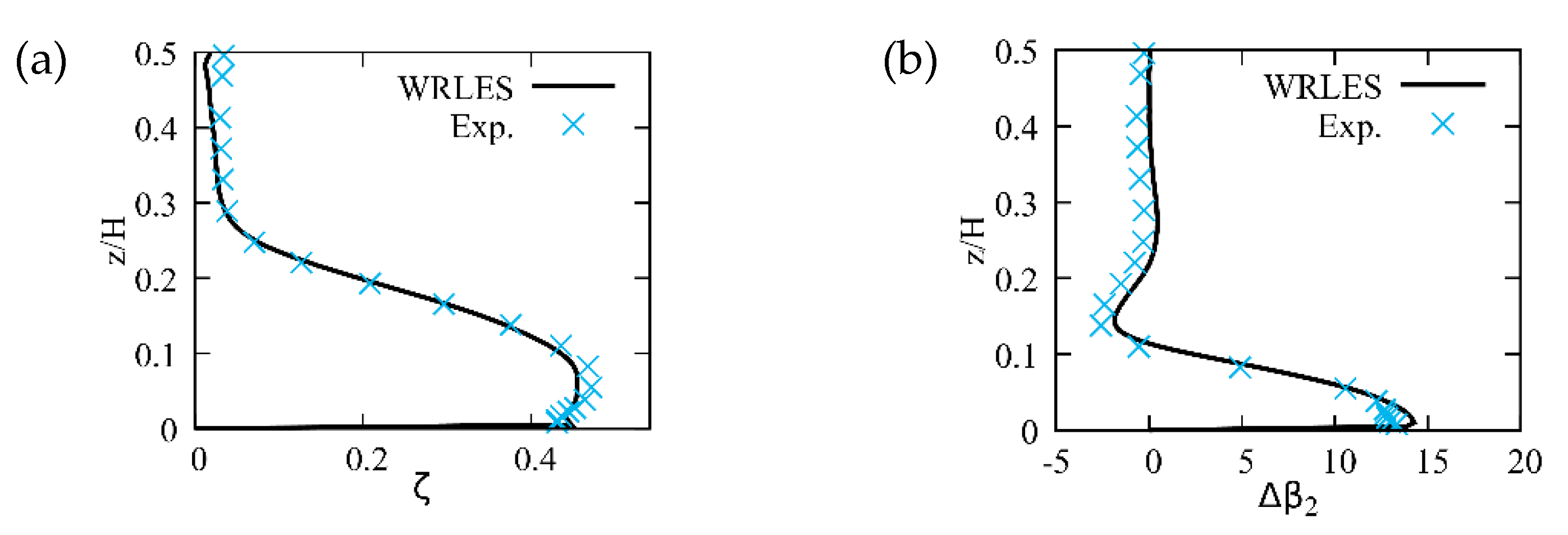
3.4.2. Validation of WRLES with Respect to Experimental Data

Further validation is now performed with experimental data for ${\mathrm{Re}}_{\mathrm{c}}=3\cdot {10}^5$, matching the configuration of Krug et al. [23]. Figure 9 presents a comparison of the pressure coefficient at the endwall. Overall good agreement is found, with pressure isolines showing similar distributions. A pressure minimum at the tip gap somewhat larger in size is obtained in the present numerical simulations, but measuring at such a position is not free of error. Beyond the position of this pressure minimum, the TLV departs from the blade $\left(\mathrm{x}/{\mathrm{C}}_{\mathrm{x}} \approx 0.3\right)$, still remaining relatively close to the blade. Between the blades, pressure isolines exhibit a mirrored S-shape. The reason for this is the TLV, as stated in [23,37,38]. This was confirmed by looking at the pressure in planes perpendicular to the blades’ camberline. It exhibits a minimum at these positions matching the location of the TLV.

Lastly, total pressure losses and flow angle deviation are compared in Figure 10. Overall, very good agreement is obtained, with a slightly higher deviation in the simulation. This slightly overprediction of WRLES with respect to the reference has also been highlighted in the previous section and may be related to modelling uncertainties affecting the boundary layer state towards the TE.

Finally, it is noted that the results obtained with the two Reynolds numbers, besides the expected differences in magnitude, in both cases feature practically the same size of the region influenced by the secondary flow, approximately $\mathrm{z}/\mathrm{H}\approx 0\dots 0.25$. Hence, it appears that the size of the secondary flow region is not dependent on the Reynolds number.

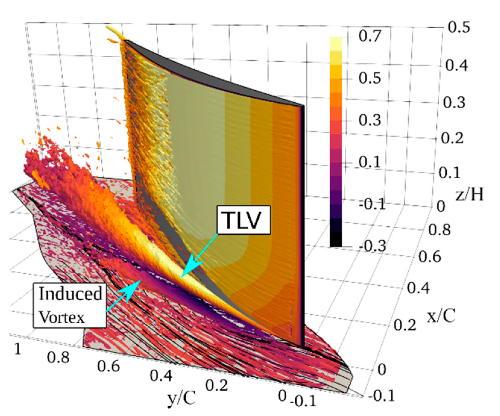
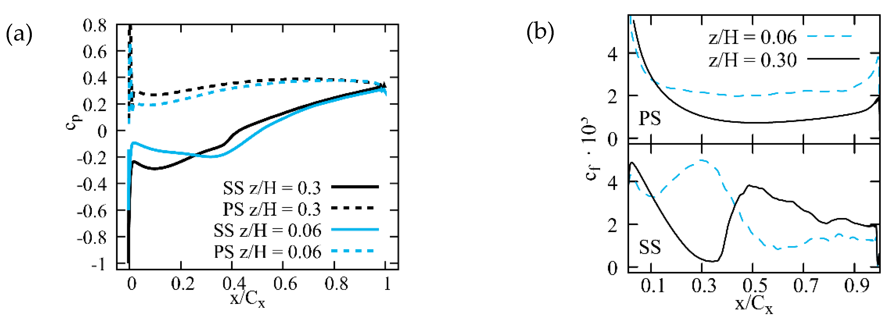
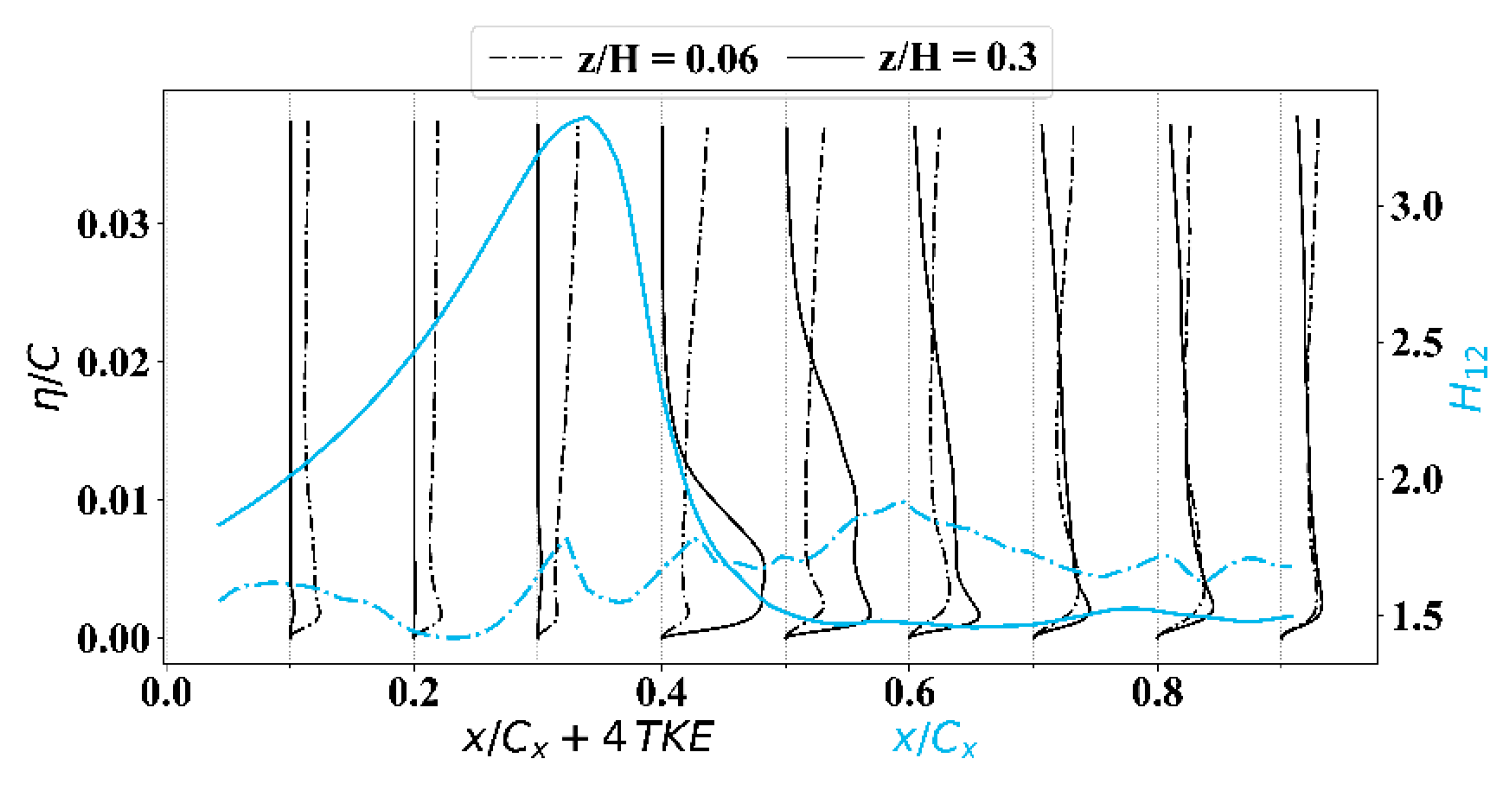
3.4.3. Secondary Flow Effects in Compressor Cascade

The overall vortical structure of the flow in this configuration is visualized through isocontours of ${\mathsf{\lambda }}_2(\langle \overrightarrow{\mathrm{v}}\rangle )=-2$ in Figure 11. The dip in the pressure isolines within the passage shown in Figure 9 matches with the trajectory of the TLV identified through ${\mathsf{\lambda }}_2(\langle \overrightarrow{\mathrm{v}}\rangle )$. The induced vortex, that is visible by the ${\mathsf{\lambda }}_2(\langle \overrightarrow{\mathrm{v}}\rangle )$-isosurface, is not detectable through the pressure at the endwall due to its smaller magnitude.

Focusing on the blade, the aerodynamic load is mostly towards the front, Figure 12a, with an almost vanishing pressure gradient at the PS and a mild negative pressure at the SS, exhibiting a minimum towards the front. The effect of the secondary flow is to reduce the blade loading, as evidenced by the differences between the pressure coefficient on PS and SS near the blade tip ($\mathrm{z}/\mathrm{H}=0.06$) compared to the midspan region ($\mathrm{z}/\mathrm{H}=0.3$), as seen in Figure 12a. Furthermore, the local minimum at the SS for $\mathrm{z}/\mathrm{H}=0.06$ is shifted downstream. Its position is slightly downstream of the position where the TLV departs from the blade. Furthermore, the minimum in the pressure at the SS at each spanwise height coincides in position with the start of the decrease of the friction levels shown in Figure 12b. For instance, at the midspan the pressure minimum is at $\mathrm{x}/{\mathrm{C}}_{\mathrm{x}} \approx 0.1$ and the local friction maximum at $\mathrm{x}/{\mathrm{C}}_{\mathrm{x}} \approx 0.05$.

Figure 13 shows the state of the boundary layer along the SS by means of the shape factor ${\mathrm{H}}_{12}$ and by wall-normal profiles of the TKE. At the tip ($\mathrm{z}/\mathrm{H}=0.06$) the shape factor is small all along the wall. Hence, the boundary layer at this height is turbulent throughout the whole blade chord. Furthermore, no marked change in shape factor related to the departure of the TLV at $\mathrm{x}/{\mathrm{C}}_{\mathrm{x}} \approx 0.3$ is observed. The friction coefficient near the tip, shown in Figure 12b, on the other hand, exhibits a marked change. Once the TLV moves away from the blade the friction coefficient decreases by a factor of more than two. Away from the blade wall an increase in TKE is observed for $0.3\le \mathrm{x}/{\mathrm{C}}_x\le 0.4$, which is directly related to the location of the TLV. Downstream of the blade, at $\mathrm{x}/{\mathrm{C}}_{\mathrm{x}}=0.89$, these higher fluctuations are also observed around the TLV core, as seen in Figure 14.

Now turning to the blade midspan ($\mathrm{z}/\mathrm{H}=0.3$), the shape factor is much larger near the leading edge peaking around $\mathrm{x}/{\mathrm{C}}_{\mathrm{x}} \approx 0.35$ then dropping to values around 1.5. Hence, the boundary layer initially is laminar and undergoes transition to a turbulent boundary layer around at this position, which is also reflected by a minimum of the friction factor at this axial position (Figure 12b). The difference in fluctuation levels at the LE between midspan and tip region is directly related to the higher fluctuations within the incoming boundary layer. At the TE very similar profiles are observed for both spanwise positions, indicating a small influence of the TLV on the TE part of the blade. This is also observed in the pressure distribution (Figure 12a), ${\mathrm{c}}_{\mathrm{p}}$ values at the TE for both spanwise positions are similar.

The departure of the TLV results in the secondary flow influencing almost the entire pitch at the outlet plane (Figure 14), with its core located approximately at the middle of the passage pitch. The wiggly isosurfaces in Figure 11 hint towards the increased levels of turbulent fluctuations around the TLV and away from the blade.

3.4.4. Effect of Relative Endwall Motion

In a previous study, the described configuration was used to study the effect of the relative endwall motion on the flow structure through DNS at ${\mathrm{Re}}_{\mathrm{c}}=1.46\cdot {10}^4$ [35]. Due to the low Reynolds number, viscous effects are higher in this case as would be in typical applications. Once the methodology was validated, simulations were carried out at ${\mathrm{Re}}_{\mathrm{C}}=3\cdot {10}^5$ and accounting for relative endwall motion, with value $\left|\left|{\overrightarrow{\mathrm{v}}}_{\mathrm{ref}}\right|\right|\sin {\mathsf{\beta }}_{\mathrm{LE}}$ in pure pitchwise ($y$) direction.

The flow field, represented through the main vortical structures, is shown in Figure 15. Here, similar trends are observed here as in the previous study at ${\mathrm{Re}}_{\mathrm{c}}=1.46\cdot {10}^4$ [35]. Relative endwall motion induces a departure of the TLV away from the blade in contrast to the case without endwall motion (Figure 11). Still, at the lower Reynolds the TLV followed a straight path, at the current Reynolds number the TLV core follows a straight path initially, then, further downstream assumes a curved path, enforced by the main passage flow. A further effect of the relative motion is the weakening of the induced vortices.

At the cascade outlet, shown in Figure 16, the most noticeable effect of the relative endwall motion is a stratification of the flow field. The endwall motion entrains fluid in pitchwise direction thus creating a fairly uniform flow near the endwall, in terms of streamwise velocity, pressure, and flow angle, similar to the study in [35]. The TKE also becomes stratified, with lower levels towards the endwall due to the imposed shear generated by the relative motion. As a result, these quantities mostly vary in spanwise direction (i.e., z-direction). Furthermore, the stratification of the velocity leads to a redistribution of the pressure losses, which are more evenly distributed and exhibit a smaller peak, compared to the case without relative endwall motion. The trends described here for the linear cascade match those observed in the rotating ring cascade in Figure 3. Despite the lower peak values, the pitchwise averaged total pressure losses reveal that the relative motion lead to overall higher losses near the wall and slightly lower losses between the peak and the midplane ($0.1\le \mathrm{z}/\mathrm{H}\le 0.25$). Lastly, both cases, with and without relative motion, show the secondary losses to be of relevance up to $\mathrm{z}/\mathrm{H}\approx 0.25$, thus indicating that with and without relative endwall motion secondary flow effects are of relevance up to similar spanwise positions. In the previous study at ${\mathrm{Re}}_{\mathrm{c}}=1.46\cdot {10}^4$ [35], a similar spanwise behavior was found. Hence, the size of the region influenced by secondary losses is not dependent on the Reynolds number nor on the relative motion.

3.4.5. Incoming, Periodically Perturbed Flow Field

A further point of interest is the effect an inflow perturbed inflow perturbed by wakes may have on the blade performance characteristics. Here, in particular, similarities and differences between the blade tip region (near the endwall) and the midspan region will be addressed. To this end a WRLES featuring a perturbed inflow was conducted. The periodic perturbation corresponded to wakes of 2 mm circular bars, as used in the corresponding experiment [23]. The instantaneous fluctuations were provided to the present authors by Wissink and Rodi from their simulation of a circular cylinder [39]. The wake was then superimposed to the instantaneous flow field of the turbulent boundary layer flow and introduced at the domain inlet. The flow perturbation had a frequency with a Strouhal number $\mathrm{Sr}=1.56$. For this particular frequency a wake moves half of the blade chord in streamwise direction while it traverses the whole pitch in pitchwise direction. Hence, for a particular phase of the period, two wakes affect the flow within a single blade passage. The effect of the inflow perturbations on the blade performance is characterized here by the phase averaged pressure and friction coefficients, depicted in Figure 17.

Phase averages were computed as ensemble averages over the bar passing period. Overall the pressure coefficient in Figure 17a shows increasing unsteadiness towards the TE, depicted through the shaded regions in the figure. This indicates a higher sensitivity of the flow at the TE with respect to the incoming wakes. Additionally, fluctuation levels are slightly higher towards the blade tip ($\mathrm{z}/\mathrm{H}=0.06)$ than at the midspan region $\left(\mathrm{z}/\mathrm{H}=0.30\right)$. Hence, periodic disturbances affect the blade loading over the entire blade span. This phenomenon observed for the compressor stage is also observed in the turbine cascade, as discussed in Section 5.4.2 below.

Considering the friction coefficient, the opposite trend is found. Near the blade tip incoming wakes have a reduced influence. In contrast, in the midspan region the end of the boundary layer transition point is directly influenced by the incoming wakes, moving backwards as the wake sweeps the blade suction side, indicating an influence of the periodic perturbances on the transition to turbulence. Furthermore, at the second half of the blade chord fluctuations are more prominent at the midspan region. In contrast, a direct influence of periodical inflow perturbations on the friction levels at the hub of a turbine stator is given and explained in detail in Section 5.4.2. This demonstrates that, in the region near the blade tip the TLV imposes the flow dynamics and “shields” the blade from the periodic perturbations.

3.5. Work in Progress

The work presented here is focused on increasing the physical and modelling complexity in the study of axial gas turbine compressors, with particular emphasis on the secondary flow. Further work involves moving towards geometries with cylindrical symmetry, i.e., annular blade rows, and increasing the modelling effort by employing wall models in the LES.

4. Sub-Project C – Periodically Transient Near-Wall Flow in the T106 Turbine Row

4.1. Scope of Sub-Project C

Sub-project C deals with far-reaching aspects of endwall flow in a low-pressure turbine cascade at realistic flow conditions (M_exit,th = 0.59, Re_exit,th = 2 × 10⁵). The basis of the investigation comprises measurements in the High-Speed Cascade Wind Tunnel (HGK) of the Institute of Jet Propulsion at the Bundeswehr University Munich [40]. URANS simulations provide additional information in areas of limited accessibility and in return, the measurements are utilized to evaluate the computational approach. A major focus is put on the different effects on endwall flow, caused by unsteady inflow conditions, changing inlet endwall boundary layer conditions, and blade loading. In this context, particular attention is given to the components of endwall loss development inside the blade passage and the downstream secondary flow field. Furthermore, an additional goal of sub-project C is investigating the aspect of endwall heat transfer.

4.2. Experimental Setup

The present investigations are conducted using a linear cascade design of the T106A low-pressure turbine profile, which was specifically developed for experimental endwall flow investigations at high-speed conditions and unsteady inflow. The periodically incoming wakes are generated by moving bars with a diameter of 2 mm, i.e., 111% of the T106 trailing edge diameter. The moving bar plane, which runs parallel to the blade passage inlet plane, is located 86% C upstream of the blade leading edge. The ratio of bars to blade count is two-to-one, i.e., P_b/P = 0.5 and the bar speed is v_b = 20 m/s. The resulting flow conditions are listed in

Table 3. T106A linear turbine cascade.

Geometric Parameters:
Chord length C	100 mm
Pitch-to-chord ratio P/C	0.799
Aspect ratio H/C	1.31
Flow Conditions:
Mach number at exit ${\mathrm{M}}_{\mathrm{exit},\mathrm{th}}$	0.59
Reynolds number at exit ${\mathrm{Re}}_{\mathrm{exit},\mathrm{th}}$	$2\cdot {10}^5$
Design inflow pitch angle ${\mathsf{\beta }}_1$	127.7°
Design outflow pitch angle	26.8°
Turbulence intensity TI	6.8%
Unsteady Inflow Conditions:
Strouhal number Sr	0.66
Flow coefficient φ	3.8

, including Strouhal number Sr and flow coefficient φ, which describe the number and orientation of wakes present in the blade passage at any given instant.

Previous experimental and numerical studies of the T106A turbine cascade have shown that increased bar velocity (higher Sr and lower φ) results in intensified effects on the secondary flow [41]. However, within a reasonable range of unsteady inflow parameters, the observed trends remain unchanged. Furthermore, when keeping a constant value of Strouhal number by varying the bar speed proportionally to the bar pitch, the influence of the flow coefficient is relatively minor. Therefore, the present investigation on loss generation is highly relevant for a wide range of unsteady inflows, including more realistic high-Sr-low-φ-cases. The design of the particular turbine cascade was mainly motivated by an unfavorable aerodynamic circumstance in previous experimental setups [42,43,44]. The issue arises from a gap, needed for the moving bar wake generator, between the wind tunnel and the cascade endwalls, upstream of the blade passages. Due to a negative pressure gradient a leakage flow is formed in the bar gap. While the freestream flow remains unaffected, it is acting as a suction on the endwall boundary layer, ultimately leading to weak secondary flow in measurements, RANS simulations and DNS, which were compared in cooperation with sub-project B [31,32].

Compared to a conventional turbine cascade, the present design, which is discussed in detail in [45], delivers several improvements regarding aerodynamics and integration of measurement techniques. The main feature is an integrated flat plate at part-span which serves as a turbine cascade endwall and provides well defined, and adjustable, inlet endwall boundary layer conditions. The flat plate is split into two parts, one upstream and one downstream of the moving bars, which generate the unsteady inflow conditions. Integrating the flat plate at part-span divides the overall flow channel into two spanwise sections as shown in Figure 18.

The larger main channel is used for all flow investigations, where the lower channel half near the flat plate is of particular interest. The smaller bypass channel on the other hand is not considered in the investigations. As opposed to the fixed position of the downstream plate, the upstream plate can be displaced in spanwise direction, varying the boundary layer augmentation on the aft plate. The value of $\Delta \mathrm{z}$ denotes the misalignment of the two flat plates, with $\Delta \mathrm{z}<0$ resulting in decreased inlet endwall boundary layer height, as shown by the velocity profiles in Figure 18b, along with a lower turbulence intensity peak [45].

Measurement Techniques

The HGK test facility is a continuously operating, open loop wind tunnel with a linear cascade test section. The wind tunnel itself is located inside a cylindrical pressure chamber, which enables an independent Mach and Reynolds number variation. Measurements of the turbine exit flow field were perf ormed using a five-hole-probe traverse in MP2 (cf. sub-project A), located at $34\% \mathrm{C}$, i.e., $40{\% \mathrm{C}}_{\mathrm{x}}$ downstream of the blade passage. A single blade pitch centered around the trailing edge extension is covered over the full blade span in the field traverse. The closest wall distance is z = 3.5 mm or equally z/H = 2.7%. The maximum FHP measurement errors based on linear error propagation are M_2,err = 0.0043, ζ_2,err = 0.321%, β_2,err = 0.093°, and α_2,err = 0.14°. All integral values of the experimental and CFD data refer to a mass-flow-weighted-average. Inlet boundary layer measurements were conducted using a CTA-probe with a tungsten wire of 1.25 mm length and 5 μm diameter. The sampling time is set to 5 s at a rate of 60 kHz. The velocity calibration was performed in a range of 0.0 ≤ M ≤ 0.5 at constant angles of pitch, yaw, and pressure levels with respect to the ensuing measurements. The overall uncertainty estimate of a velocity sample is Δv ≤ 2.5 m/s. Further details on the experimental setup, measurement techniques, the particular turbine cascade design, which was implemented, and a discussion of the full experimental results can be found in [45].

4.3. Numerical Setup

The numerical simulations were performed using the URANS flow solver TRACE by DLR with the $\mathrm{k}-\mathsf{\omega }$ turbulence model by Wilcox [46] and ${\mathsf{\gamma }\mathrm{Re}}_{\mathsf{\theta }\mathrm{t}}$ transition model by Langtry and Menter [47]. The computational domain shown in Figure 19 covers a single blade pitch with periodic boundary conditions. It is divided into an upstream block group encompassing the front plate, the moving domain containing two bar pitches, and a downstream block group which encompasses the blade passage and aft plate.

Due to the asymmetric geometry caused by the integrated flat plate, the full blade span including the lower bypass channel is resolved in the computation. The blade passage is discretized using an OCGH-topology and low-Reynolds wall treatment (y⁺ ≤ 1), resulting in high boundary layer resolution. Sufficient spatial and temporal discretization is ensured by a sensitivity study, which leads to an overall number of nodes of approximately $8\cdot {10}^6$ and a number of time steps per moving domain period of 800. Leakage panels are incorporated at the bar gap boundaries to simulate the leakage flow. The imposed static pressure condition is determined based on experimental data. The flow conditions prescribed at the in- and outlet plane match the wind tunnel conditions in the experiment (${\mathrm{M}}_{\mathrm{exit},\mathrm{th}},{ \mathrm{Re}}_{\mathrm{exit},\mathrm{th}}= \mathrm{f}\left(\mathrm{T}t1, \mathrm{p}t1, \mathrm{p}3\right)$ and ${\mathrm{TI}}_1$). A detailed description of the computational approach can be found in [48].

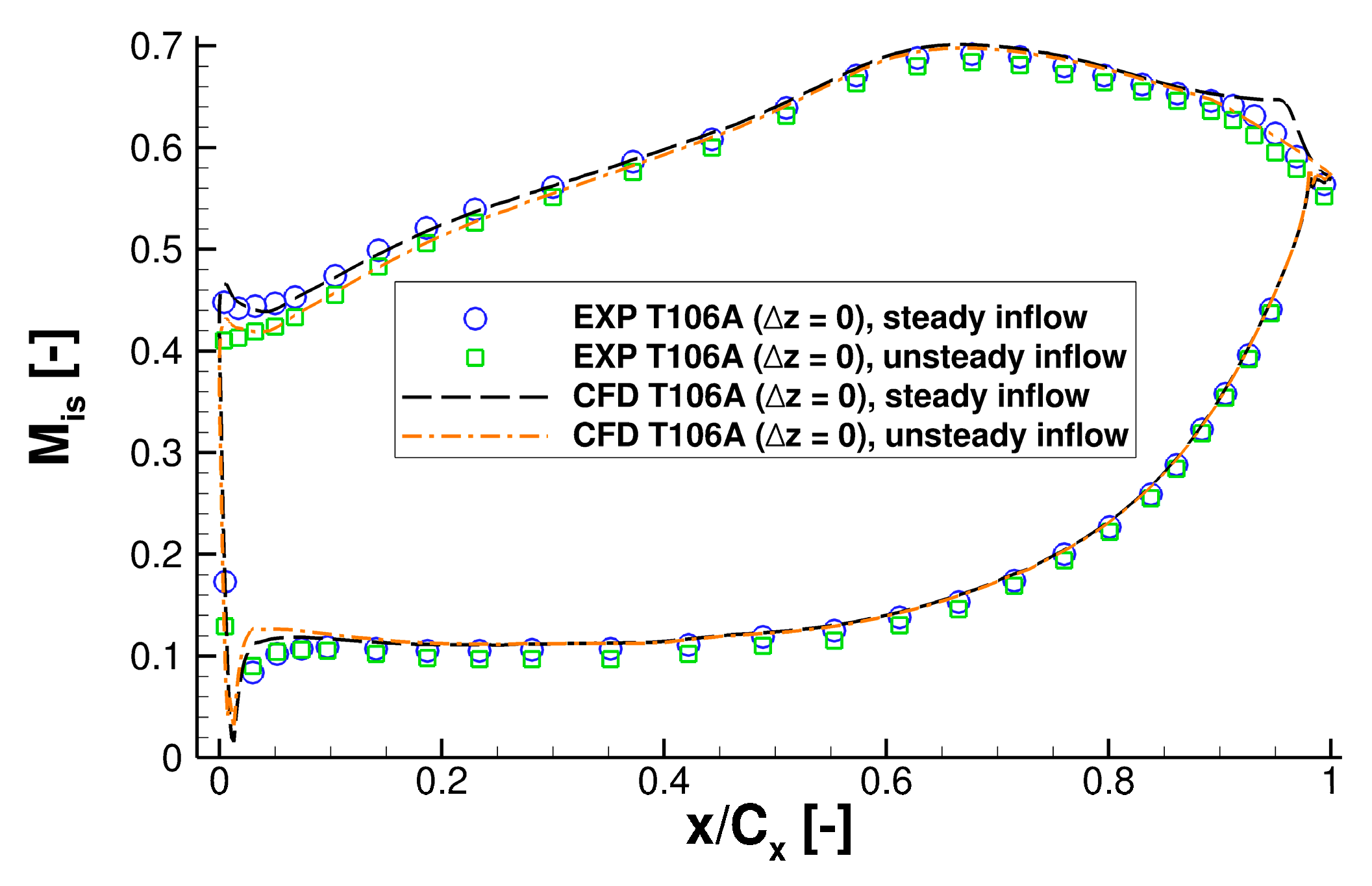
4.4. Current Investigations and Results

The isentropic blade Mach number distribution at midspan, shown in Figure 20, is the most important gauge for evaluating the numerical prediction of the 2D turbine cascade flow.

The T106A is a predominantly aft-loaded profile which features a very small separation bubble at the investigated steady inflow conditions (see Table 3), caused by the adverse pressure gradient in the aft section of the blade suction surface. The numerical predictions match well with the measured distribution except for a more pronounced separation bubble in the CFD, located at approx. x/C_x = 0.95. This discrepancy is attributed to a quicker turbulence decay in the computational domain resulting in a locally lower turbulence intensity, even though ${\mathrm{TI}}_{1, \mathrm{CFD}}$ matches the experimental level. The turbulent dissipation rate could be adjusted by tweaking the inlet level of the turbulent length scale, however, a low level of this quantity is imperative for an accurate prediction of the loss generation. In the case of unsteady inflow conditions, a pitchwise incidence of $\mathrm{i}=-1.5°$ is induced, resulting in decreased blade loading in the front part of the blade suction surface. At the aft section of the suction surface the separation bubble is suppressed due to wake induced transition. Both these effects are predicted well in the numerical simulations [48].

The level of secondary flow and the effects of the incoming wakes as well as the inlet boundary layer variation by flat plate misalignment are gauged by field measurements of the turbine exit flow in MP2. The results are illustrated over the entire channel height in Figure 21 and as spanwise distributions of pitchwise-average values in Figure 22.

The secondary outflow angle $\Delta {\mathsf{\beta }}_{2, \sec }$ and the secondary total pressure losses ${\mathsf{\zeta }}_{2, \sec }$ are defined by

$${\Delta \mathsf{\beta }}_{2,\sec }={\mathsf{\beta }}_2-{\overline{\mathsf{\beta }}}_{2,\mathrm{MS} }$$

(4)

$${\mathsf{\zeta }}_{2,\sec }={\mathsf{\zeta }}_2-{\overline{\mathsf{\zeta }}}_{2,\mathrm{MS} } \mathrm{with}$$

(5)

$${\mathsf{\zeta }}_2=\frac{{\mathrm{p}}_{\mathrm{t}1}-{\mathrm{p}}_{\mathrm{t}2}}{{\mathrm{p}}_{\mathrm{t}1}-{\mathrm{p}}_3}$$

(6)

It is apparent that the different inlet endwall boundary layer conditions result in varying degrees of secondary flow in the lower channel half near the integrated flat plate. The case of Δz = 0, representing the thickest boundary layer, exhibits the strongest secondary flow. Lowering the inlet boundary layer thickness in the cases of Δz = −1% C and Δz = −2% C, results in a reduction of peak values of over-/underturning as well as secondary losses. Additionally, the regions of secondary losses and over-/underturning are shifted towards the endwall. This is caused by a less pronounced liftoff of the passage vortex.

Comparing the turbine exit flow in cases with steady and unsteady inflow, it is apparent that the periodically incoming wakes also cause an attenuation of the time-averaged secondary flow. In Figure 22, it is particularly noticeable that the reduction in time-averaged peak values of ${\mathsf{\zeta }}_{2,\sec }$ and ${\Delta \mathsf{\beta }}_{2,\sec }$ as well as the spanwise shift by means of unsteady inflow conditions is very similar to the effect of decreasing the inlet endwall boundary layer height, especially in the underturning region.

Although not shown here, the numerical simulations offer a good prediction of the spanwise distributions as well as the effects of unsteady inflow and endwall boundary layer variation [48]. A slightly narrower region of elevated secondary losses in combination with an overshoot of the loss peak is commonly observed in numerical simulations solving the URANS equations with an eddy-viscosity model. The important quantity of overall losses, defined here as integral half-span losses, are predicted with very good accuracy by the simulations, e.g. in the Δz = −1% C case ${\left({\mathsf{\zeta }}_{2, \mathrm{HS}}\right)}_{\mathrm{EXP}}=4.7\%\approx {\left({\mathsf{\zeta }}_{2, \mathrm{HS}}\right)}_{\mathrm{CFD}}=4.6\%$. For this specific comparison, the CFD value was integrated only within the experimentally accessible area of $0.027\le \mathrm{z}/\mathrm{H}\le 0.5$.

For a further description of the effect of periodically incoming wakes, the numerical predictions of the time resolved flow field in MP2 is shown at two distinct times in Figure 23. In order to evaluate the effects of incoming wakes on the blade passage loss generation, the integral losses in Figure 23a are corrected by subtracting the time-averaged values upstream the blade passage $\Delta {\mathsf{\zeta }}_2={\mathsf{\zeta }}_2-{ \mathsf{\zeta }}_{{\mathrm{x}}_{\mathrm{ref}}}$. The first time resolved flow field at $\mathrm{t}/{\mathrm{T}}_{\mathrm{BP}}=0.125$ corresponds to the maximum overall losses (integral over half span) in the moving bar period ${\mathrm{T}}_{\mathrm{BP}}$. Around this instant, the remains of an incoming bar wake, which has been subjected to stretching and bowing in the blade passage, first interact with the passage vortex in MP2. Moments later, the bar wake travels in pitchwise direction, where it affects the blade suction surface and ultimately overlaps with the blade wake at y/P=0.5 which corresponds to the extension of the blade trailing edge. This leads to a very wide blade wake and maximum pitchwise-averaged midspan losses. Considering the definition of the secondary losses, the peaks of midspan and overall losses occur around the same time as the secondary loss minimum.

This is confirmed by the streamwise vorticity plot in Figure 23d, where a temporary attenuation of the passage vortex can be seen. The reduced liftoff of the secondary vortex system correlates with a less distinct horseshoe vortex pressure side leg, which has already begun to merge with the passage vortex in MP2. The same observation is made in the low-speed annular cascade adaptation of the T106A in sub-project D (see Section 5.1). The second instant at $\mathrm{t}/{\mathrm{T}}_{\mathrm{BP}}=0.7$ exhibits further pitchwise distance between the bar wake and the blade wake in MP2, so there is no overlapping. Additionally, bar wake induced transition forces a temporary suppression of the separation bubble on the blade suction surface. These combined circumstances result in a very narrow blade wake and relatively low levels of corrected midspan, overall, and secondary losses around this instant, even falling below the steady state. When evaluating a time resolved downstream flow field, it is important to understand that the local flow properties are not only influenced by the bar wake in that specific location, but especially by upstream interactions with the blade passage flow. The level of disturbance of the turbine exit flow during a moving bar period, originating upstream, is reliant on the unsteady inflow conditions, defined by Strouhal number Sr and flow coefficient φ. Since multi-row axial turbines usually operate at much higher Strouhal numbers it is safe to assume that the passage flow is constantly in a state of varying disturbance.

After investigating the secondary flow in MP2, where unsteady inflow conditions and changing inlet boundary layers showed similar time-averaged effects, questions arise as to the upstream endwall flow development and corresponding loss generation throughout the blade passage. Comparing the time-averaged axial change in non-dimensionalized entropy in Figure 24 in case of unsteady inflow conditions to the steady state shows an accelerated overall loss increase in the front part of the blade passage. This is caused by increased blade profile losses due to the perturbation of the blade surface boundary layers by the incoming bar wakes with high levels of turbulence. Unlike the profile losses, the secondary loss generation is not increased by the incoming wakes inside the blade passage ($0\le \mathrm{x}/{\mathrm{C}}_{\mathrm{x}}\le 1$). In fact, the interaction of the wakes with the endwall boundary layer in the front part of the passage delays the roll-up of the passage vortex and its pressure-driven translation towards the suction surface, which leads to an attenuation of the secondary loss further downstream. Outside the near-endwall region, the incoming wakes periodically force an earlier turbulent transition on the blade suction surface, which leads to the suppression of the separation bubble.

Therefore, the rapid increase of the profile losses near the trailing edge ($\mathrm{x}/{\mathrm{C}}_{\mathrm{x}}=1$) in the steady case is attenuated by the unsteady inflow conditions. In sum, the steady case level of overall losses is catching up to the unsteady inflow case and the entropy lines converge with further distance downstream of the blade passage. Thus, despite the flow field changes, seen in MP2 (Figure 22 and Figure 23), the effect of the periodically incoming wakes on the time-averaged integral losses in the turbine exit flow is very small. This finding is consistent with the total pressure field measurements [45] as well as DNS of a previous T106A cascade [31,32].

Overall, the effect of unsteady inflow conditions can be summarized as a spatial redistribution of the loss generation with a premature loss increase due to wake interaction with the blade surface boundary layer followed by attenuation of the profile- and secondary loss generation in the aft-section of the blade passage. A more comprehensive analysis of the secondary flow development and the local sources of loss inside the blade passage can be found in [48]. Contrary to the axially varying effect of unsteady inflow conditions, decreasing the inlet endwall boundary layer height results in a nearly constant reduction of the endwall loss generation, beginning around the midpoint of the blade passage where the secondary flow is formed. Lastly, the effect of increased frontal blade loading leads to a rise in profile losses in the front part of the passage followed by increased secondary losses due to stronger transverse pressure gradients [49].

4.5. Work in Progress

Upcoming work in sub-project C includes expanding the experimental data set with time-resolved measurements and optical measurements. A particular area of interest is the secondary flow interaction with the blade suction surface flow. Additionally, great effort is being invested in an investigation of the aspect of endwall heat transfer. This goal is planned to be achieved by deploying the progressive measurement technique of ultra-high-speed temperature sensitive paint on the cascade endwall surface. The capability of this measurement technique has recently been verified successfully on a flat plate with a frame rate of up to 40 kHz.

5. Sub-Project D—Influence of Periodic Wakes on the Transient Near-Wall Flow in an Annular Axial Turbine Cascade

5.1. Scope of Sub-Project D

Especially in a LPT environment, periodic flow perturbations induced by rotor-stator interaction exert pronounced consequences on the blade profile boundary layers, which are inherently unstable and prone to separation due to the high LPT stage loading and the prevailing low Reynolds numbers [50]. Despite decades of highly accurate, profound research addressing the different aspects of rotor-stator interaction, a deeper physical understanding regarding the highly unsteady interplay of the transported wake structures, the involved boundary layers and the blade row’s secondary flow system is still sought.

Therefore, in sub-project D, experimental investigations in a large-scale annular test rig for the time-resolved analysis of wake-stator BL flow interaction within a turbine environment are conducted. This way, the influences of curvilinear endwalls, non-uniform, radially increasing pitch and radial flow migration are incorporated, increasing the degree of complexity over linear setups. The modified stator blade profile, labeled as T106^RUB, was developed within this collaborative project for matching the transition and separation characteristics of the original T106 profile (also applied in sub-project C) at low flow speeds, thus facilitating measurements to be taken in an annular, large-scale test rig (see [51]). The stator flow is periodically perturbed by incoming wakes from a rotating wake generator.

The aim of the current activities is to establish a connection between the incoming, periodically wake-perturbed flow field, the highly-unsteady situation in the stator blade row (stator profile and passage flow) as well as the exit flow containing the secondary flow structures in an annular LPT environment. For this, multiple measurement techniques upstream, within the stator blade row and downstream are connected to provide an extensive set of experimental data. This allows to study the unsteady behavior of the boundary layers developing on the LPT stator profiles and their effect on secondary flow patterns under the influence of periodic inflow perturbations. The transition phenomena occurring in the profile boundary layers are investigated under both unperturbed and periodically perturbed inflow by means of spectral analysis, the semi-quantitative characterization of the wall-stress system and an evaluation of the statistic quantities. Using experimental hot-film data from different positions of blade span, the BL flow behavior can be linked to the temporal evolution of the secondary flow structures, which is assessed with the help of temporal and spatially highly resolved flow field traverses downstream of the blade row in focus. To the best knowledge of the authors, until today only a few studies were presented, comparing appropriate time-resolved data from the midspan section with data from the near-wall region, where secondary flow effects have to be considered. Ultimately, the acquired measurement data provide highly resolved validation data for accompanying URANS and LES computations.

The presented investigations give a brief outline of key findings from recent publications by the authors, where the unsteady impact of periodic bar wakes on the flow field downstream of the stator row as well as on the stator profile pressures and boundary layers were discussed. For details, please see [51,52,53,54,55,56,57,58].

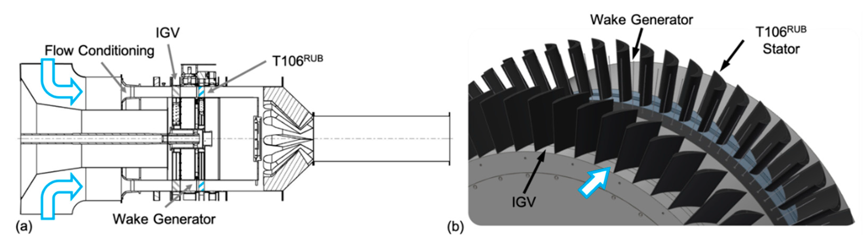
5.2. Experimental Setup

The experimental activities described in this contribution were carried out in the large-scale, axial flow turbine test facility Axial Turbine II at the Chair of Thermal Turbomachines and Aeroengines of Ruhr University Bochum. The facility was designed to allow highly resolved measurements of the unsteady interaction between the stator profile flow and periodically impinging wake structures within an annular setup. For this purpose, the test rig was used in a 1.5 stage configuration with an IGV row, a rotating wake generator and the T106^RUB stator row under investigation, presented in Figure 25. The large dimensions of the flow channel allow detailed flow measurements with negligible perturbation by installed probes. Rotatable casing elements with multiple probe accesses facilitate the recording of two-dimensional flow field traverses in various planes. Following, the most important information regarding the setup are given, a more detailed description was provided in [51,52,53].

Following a combination of flow straightener cells, a turbulence grid and a contraction for generating uniform inflow within the settling chamber, the flow passes an IGV row (NACA 8408 profiles) to ensure proper inflow angles to the T106^RUB stator whilst leaving the flow as far as possible unaffected by wakes and secondary flow. With both 60 IGV and T106^RUB profiles, it is ensured that every T106^RUB passage faces identical inflow conditions. The IGV is placed 261% C upstream of the wake generator.

To simulate the unsteady rotor-stator interaction of an axial turbomachine, the rotor disk between the IGV and the T106^RUB stator was equipped with radially stacked, circular steel bars (bar diameter D_b = 2 mm, bar length L_b = 168 mm). The use of periodically passing circular bars facilitates to isolate both velocity defect and turbulence increase of typical rotor blade wakes without the secondary flow structures emerging in a real rotor passage. Wakes are generated at an axial distance of 33% C upstream in a plane parallel to the stator leading edges, representing a typical axial gap width in a LPT. The investigations were carried out for a bar pitch of P_b = 78 mm, matching the pitch of both the IGV and the T106^RUB.

The aft-loaded blade profile (cylindrical geometry) under investigation, labeled as T106^RUB, is an in-house modification of the well-known T106 LPT blade, with modified distributions of profile thickness and curvature. It was developed to match Reynolds number, blade loading distribution c_p at midspan and thus an equivalent boundary layer development of the original T106 profile at the rig’s low Mach number flow. The principles of the transformation procedure were described by Sinkwitz et al. [51].

The test facility is operated with ambient air, continuously in an open circuit. Flow is induced by a 150 kW variable speed engine coupled to a radial blower providing a mass flow capacity of $\dot{\mathrm{m}}\approx 13 \mathrm{kg}/\mathrm{s}$. To avoid inflow perturbations, the blower is placed downstream of the test section, thus the rig is operated in suction mode.

Table 4. Main test rig properties and turbine stage parameters.

Test Rig		Turbine Stage
Outer diameter (Casing)	1660 mm	Chord length IGV	137 mm
Inner diameter (Hub)	1320 mm	Stagger angle IGV	−25.5°
		Chord length T106RUB	100 mm
		Stagger angle T106RUB	30.7°
		Blade count IGV, T106RUB	60
Operating Point, Design Point		Design Flow Angles, Midspan
Mass flow $\dot{\mathrm{m}}$	12.8 kg/s	IGV inlet ${\mathsf{\alpha }}_0$	90.0°
Reynolds number at exit ${\mathrm{Re}}_{\mathrm{exit},\mathrm{th}}$	$2\cdot {10}^5$	IGV outlet = ${\mathsf{\alpha }}_1$ T106RUB inlet ${\mathsf{\alpha }}_2$	52.3°
Mach number at exit ${\mathrm{M}}_{\mathrm{exit},\mathrm{th}}$	0.091	T106RUB outlet ${\mathsf{\alpha }}_3$	153.2°

summarizes the most important details.

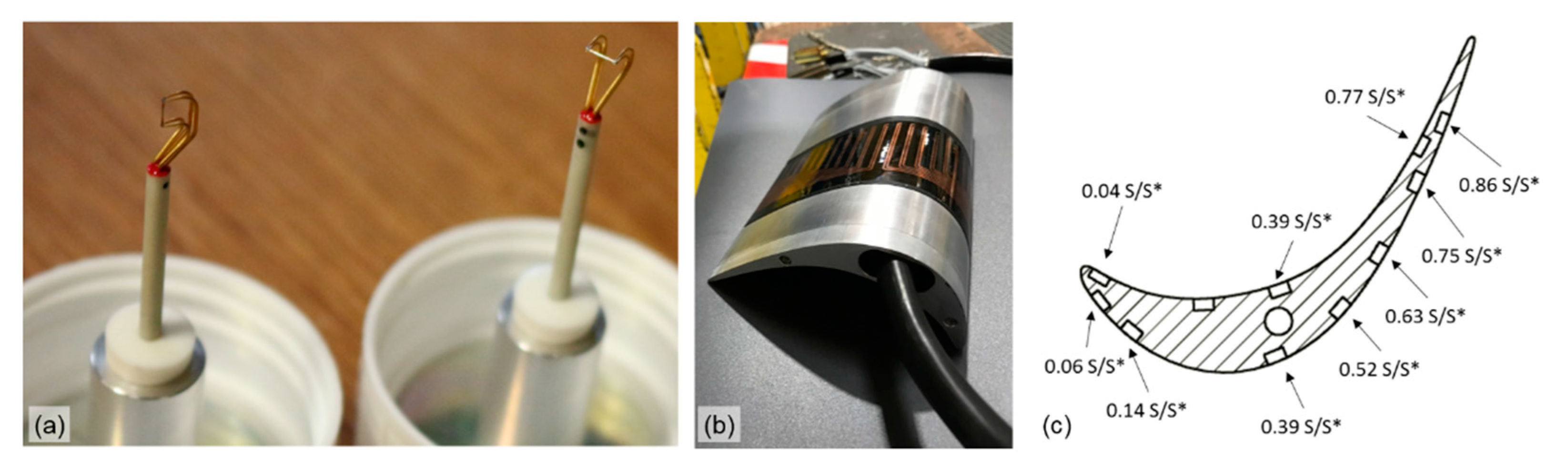
5.3. Measurement Techniques

Monitoring of the operating point was realized with Prandtl-probes at different characteristic planes and a combined temperature/humidity sensor at the rig inlet. A detailed description of the applied transducers and devices is provided in [51,52,53,54].

To quantify the bar wake impact on the stator flow and the resulting secondary flow structures, flow field traverses were carried out in relevant planes, including the axial gap between the wake generator and the T106^RUB stator and the exit flow field downstream of the T106^RUB stator. Two-dimensional flow field traverses in the exit flow (38 radial and 25 circumferential positions, distributed over two T106^RUB stator passages) have been carried out at 15% C and 35% C downstream of T106^RUB TE. For this, hot-wire anemometry measurements (CTA mode) were conducted using a Dantec Dynamics StreamLine 90N10 CTA anemometer (incorporating three 90C10 CTA modules) and both straight and slanted 1-wire probes in the inflow and Split-Fiber probes (SFP, types 55R56 and 55R57) in the wake-flow, shown in Figure 26a. In the wake regions, characterized by intense flow angle variations, SFP have proven superior usability. Due to this and their increased durability, they have been chosen for most of the measurements. All probes were subjected to a multi-dimensional calibration prior to the measurements, during which the corresponding flow angle and velocity were varied within the anticipated range. Using the two voltage values resulting from the SFP measurement, the respective flow angle as well as the magnitude of the velocity (giving a 2D flow vector) were reconstructed. By combining two consecutive measurements with SFP 55R56 and 55R57, the phase-averaged 3D flow vector was finally reconstructed by analyzing the data sets of both probe measurements simultaneously.

For experimental data acquisition within the T106^RUB stator passage, several T106^RUB profiles were equipped with surface-mounted hot-film sensor arrays, Kulite-sensors (10 sensors of type LQ-125, sealed gage variant) and static pressure taps. Hot-films (thickness ≈ 0.05 mm, custom-fabricated by Tao of Systems Integration Inc.,) feature 24 sensor elements on the SS layout, 20 elements on the PS layout and a constant spacing of 6 mm between the individual sensor elements. For hot-film sensor operation and data acquisition also the StreamLine 90N10 CTA anemometer along with three 90C10 CTA modules was applied. For data acquisition of hot-wire and hot-film measurements, a National Instruments NI 9215 module was employed. More details regarding the hot-film setup are provided in [54].

Signals have been recorded at a rate of up to 100 kHz (550 times higher than the maximum bar passing frequency for the shown investigations), triggered by a one per revolution signal from an inductive encoder on the rotor shaft. Due to the boundary layer analysis to be evaluated in the course of the hot-film measurements and the higher statistical moments used for this purpose, a corresponding database is necessary. Therefore, for the phase averaging of each hot-film sensor-depending on the operating point/speed of the wake generator-up to 3000 samples were recorded. In this case, a sample is defined as the continuous period of 3 bar wakes. For the time-intensive measurement of two-dimensional flow fields with in part over 1000 measuring positions (SFP measurements), the number of samples inevitably had to be reduced. Nevertheless, a minimum number of 1000 samples was still maintained here.

To facilitate T106^RUB profile hot-film, Kulite and static pressure measurements in various radial (direction of blade height) positions, a modular T106^RUB blade was realized. The modular blade is made up of multiple, stackable elements and can be equipped with various instrumented modules at different blade height positions within the modular blade. In Figure 26b the assembled modular blade containing a module with SS hot-film instrumentation at midspan position is shown. Figure 26c gives the Kulite sensor locations.

5.4. Current Investigations and Results

As stated in the introduction, in multistage turbomachinery configurations, the profile flow is periodically affected by wakes of upstream profiles, perceivable by cyclical patterns regarding the flow quantities. Dependent on Strouhal number Sr and flow coefficient φ, individual components of the vortex system show a wake-induced, recurrent cycle of formation, weakening and displacement. For all investigations the same theoretical (isentropic) T106^RUB exit Reynolds number ${\mathrm{Re}}_{\mathrm{exit},\mathrm{th}}$ (based on T106^RUB chord length C and the theoretical exit velocity ${\mathrm{v}}_{\mathrm{exit},\mathrm{th}}$ analogous to sub-project C) was applied for the definition and adjustment of the operating point, defined by ${\mathrm{Re}}_{\mathrm{exit},\mathrm{th}}=2·{10}^5$ and representing a typical value for LPT operation. To study the effect of periodic flow perturbation, the conditions of unperturbed T106^RUB inflow were compared to two other cases, one with a moderate frequency of perturbation (Sr = 0.43, φ = 2.97) and another one with a high frequency of perturbation (Sr = 1.33, φ = 0.97), whereas Sr was defined with flow quantities at midspan. From the hot-wire traverses, the turbulence intensity at the T106^RUB inlet was estimated to be between TI = 0.5% in the free stream and TI = 2.5% in the IGV wake without bar wake perturbation, whereas the bar wakes induce a periodic TI increase, reaching values of it up to TI = 20%.

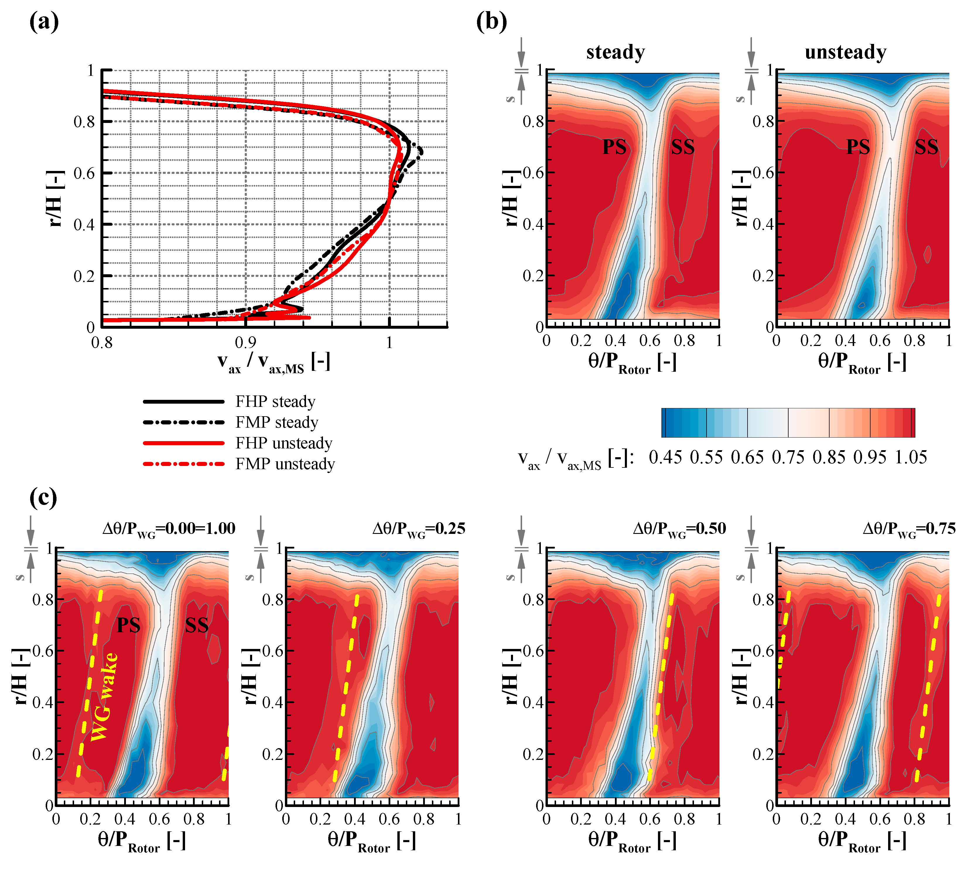
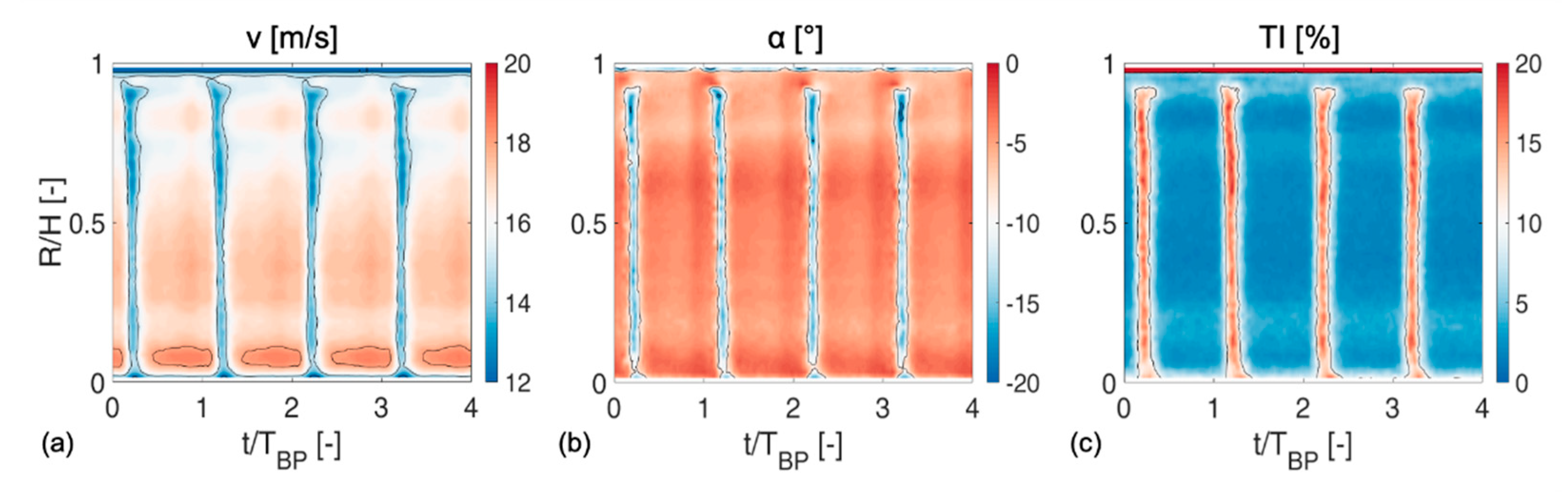
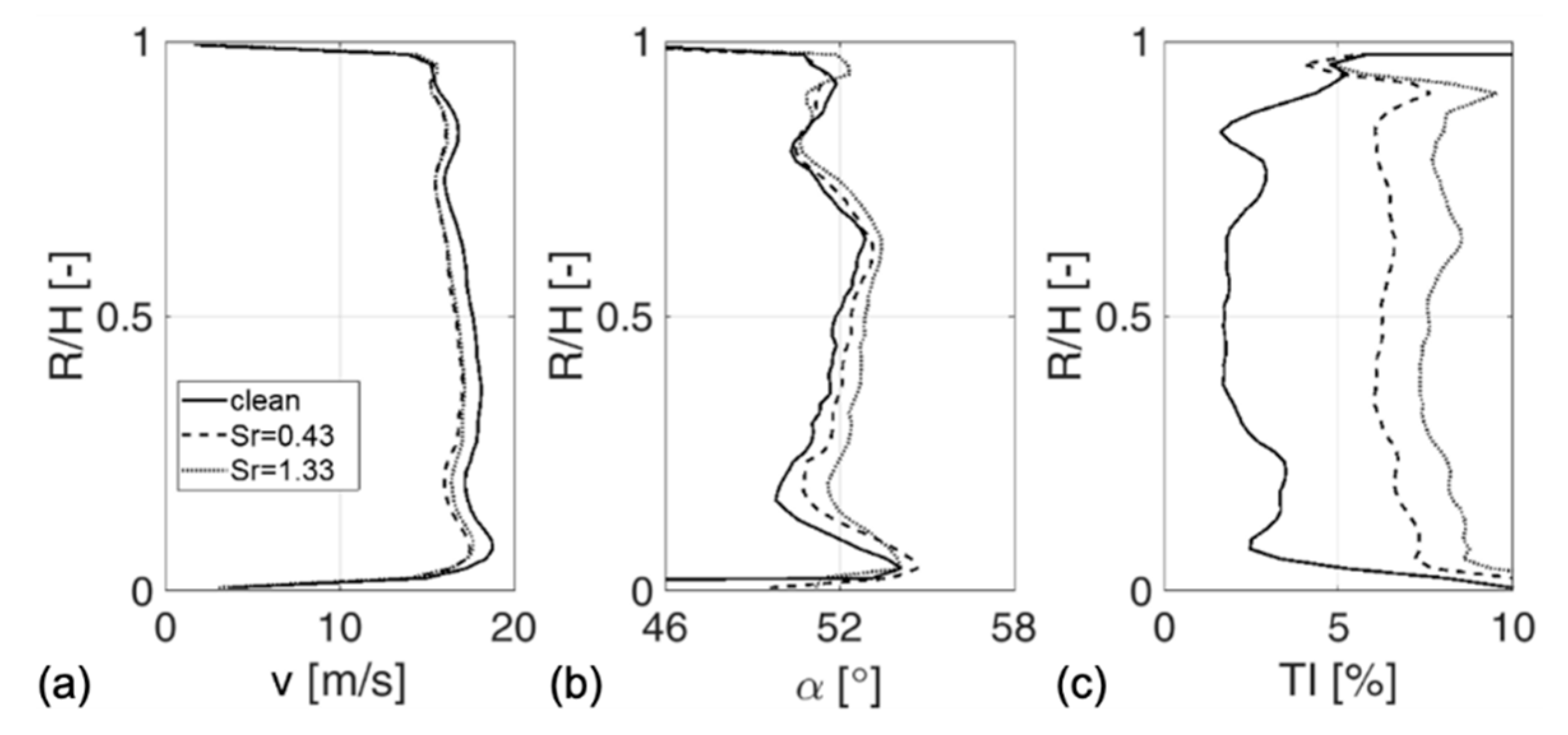
5.4.1. Incoming, Periodically Perturbed Flow Field

For the characterization of the immediate bar wake impact, Figure 27 and Figure 28 show hot-wire data, acquired in the axial gap between the wake generator and the T106^RUB leading edges with radial traverses.

Thus, in Figure 27 the temporal evolution (phase-averaged quantities) of the velocity v (a), the flow angle in circumferential direction α (b) and the turbulence intensity TI (c) over the channel height R/H are given for Sr = 1.33, φ = 0.97. From all three flow quantities, minor but still detectable remains of the IGV secondary flow structures are evident. However, much more prominent are the bar wake induced effects, causing a combination of periodic T106^RUB inflow incidence (Δα ≈ 10°), a velocity defect (Δv > 5 m/s) and a turbulence increase from the unperturbed level of TI ≈ 1.5% up to levels of TI > 15% in the midspan section. Additionally, Figure 28 gives an overview regarding the time-averaged distributions of the discussed flow field quantities for the unperturbed and the two perturbed cases. Despite the additional periodic, bar wake induced perturbations, a certain degree of homogenization for the velocity and the flow angle can be assessed concerning the IGV non-uniformities near the endwalls. In terms of turbulence intensity, the increased rotational speed of the wake generator and thus the higher relative velocities for higher Sr also increases the general level of turbulence from TI < 2% (undisturbed) to TI ≈ 8% for Sr = 1.33 at midspan.

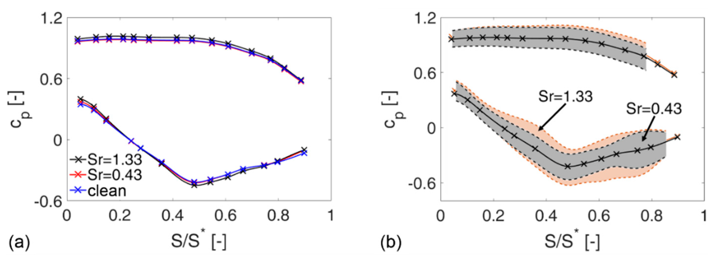
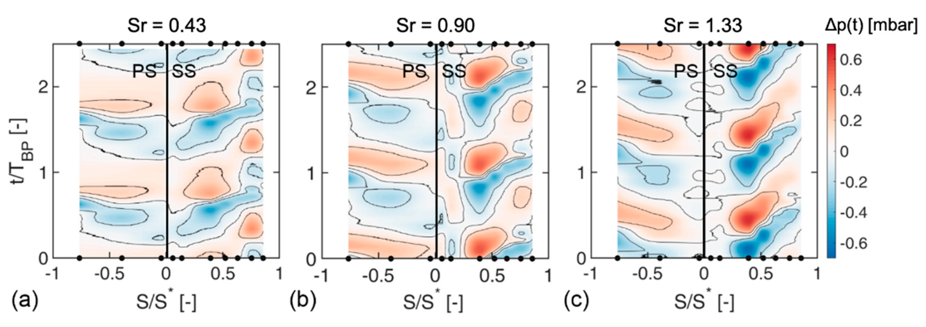
5.4.2. Situation within the T106^RUB Blade Row

Within the T106^RUB blade row, the incoming bar wakes evoke both large-scale (blade row kinematics) and micro-scale (profile boundary layer properties) effects, wherefore the following analysis is divided into two parts.

First, Figure 29 describes the impact of the periodic perturbation on the blade loading ${\mathrm{c}}_{\mathrm{p}}$ (referring to the exit state downstream of the stator row) in time-averaged view (a) and for time-resolved measurement data (b), where $\mathrm{S}/{\mathrm{S}}^{*}$ represents the proportion of the suction or pressure side length. Thus, $\mathrm{S}/{\mathrm{S}}^{*}=0$ describes the LE and $\mathrm{S}/{\mathrm{S}}^{*}=1$ the TE. The time-averaged results (a) do not exhibit prominent changes between the undisturbed and the two disturbed cases. However, employing time-resolved data from flush-mounted Kulite sensors (b), an evaluation of the extrema in profile pressures at every sensor location indicates generally increasing unsteadiness and thus progressively unsteady blade loading with increasing Sr. This increasing unsteadiness is also observed in the simulations of the periodically perturbed compressor cascade, investigates in sub-project B (see Section 3.4.5). Interestingly, despite a general reduction in fluctuation amplitudes for the lower Sr case (Sr = 0.43), close to the profile TE, the amplitudes are not reduced but feature a maximum excitation, which will be analyzed in the following.

For a time-resolved analysis of the involved phenomena, Figure 30 shows the temporal evolution of the pressure fluctuations along the T106^RUB profile at midspan for the already introduced cases (Sr = 0.43, Sr = 1.33) and an intermediate perturbation frequency (Sr = 0.90). In this depiction, $0<\mathrm{S}/{\mathrm{S}}^{*}<1$ describes the suction side flow, whereas $-1<\mathrm{S}/{\mathrm{S}}^{*}<0$ represents the pressure side flow with $\mathrm{S}/{\mathrm{S}}^{*}=0$ marking the LE. For all three cases, the periodic pressure fluctuations (as response on the bar wake convection) can be determined clearly across the profile surface, both on the pressure and the suction side. Near the suction side, the passage flow is compressed and accelerated by the approaching wake structure, so that the wake pushes a regime of accelerated flow in front of it, followed by a region of low velocity fluid, which is vice versa on the pressure side, shaping the typical, negative jet like structure of a wake within a blade passage [59,60].

A direct comparison between the three shown scenarios indicates a shift of the regions on the suction side, which are most excited by the periodic perturbation. From an exclusive major excitation centered around S/S* = 0.5 for Sr = 1.33, for decreasing Sr a weakening of this zone and a co-occurring augmentation of the periodic excitation towards the trailing edge is evident, while wake strength decreases and the time between wake events increases. The underlying phenomena, which are responsible for this behavior and take place in the profile boundary layers, are discussed on the basis of hot-film data.

For this, Figure 31 shows the time-resolved evolution of quasi wall shear stress (QWSS) along the T106^RUB suction side at midspan for the low and high Sr cases. For means of comparison, on top of the diagrams the QWSS distribution for undisturbed flow is added. The practicable quantity of QWSS is used as a qualitative means for the description of the boundary layer. Following the approach of Hodson [61], the measured voltage values (E) are combined with the sensors’ behavior under zero-flow conditions (E₀) for a semi-quantitative analysis of the wall shear stress τ_w:

$${\mathsf{\tau }}_{\mathrm{W}} ~{\left(\frac{{\mathrm{E}}^2-{\mathrm{E}}_0^2}{{\mathrm{E}}_0^2}\right)}^3=\mathrm{QWSS}.$$

(7)

Besides the already mentioned distortion of the local pressure and velocity field (negative jet effect), the connected energy transfer introduces small-scale oscillations from the highly turbulent wake flow into the boundary layer flow, increasing the wall shear stress intermittently. For Sr = 1.33 the suction side boundary layer downstream of S/S* = 0.78 alternates between a state of low (but compared to the undisturbed reference case, still slightly increased) and distinctly elevated QWSS. Obviously, the period of time between individual wake events is not sufficient enough for the boundary layer in the rear part of the suction side to fully recover, as the unperturbed state (shown above) is not reached in between individual wakes. This might be reasoned by a combination of the following aspects:

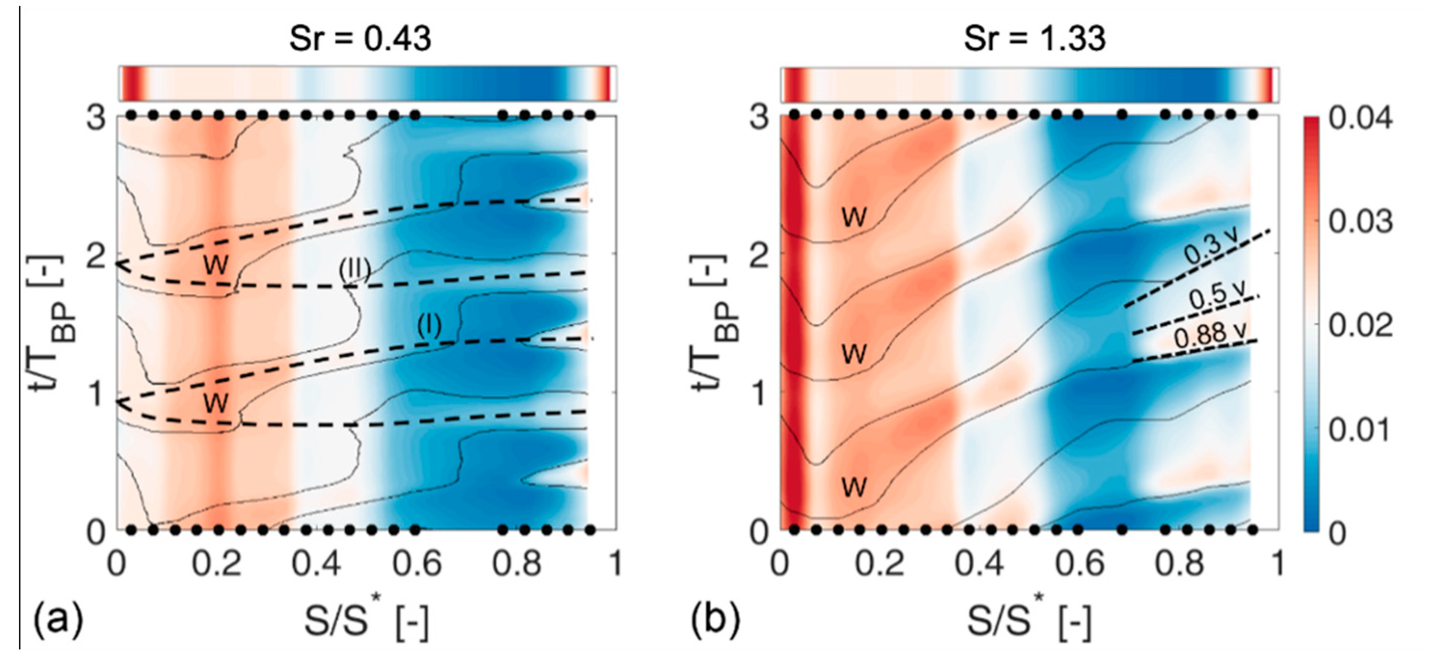
• Wake-induced boundary layer instabilities, like locally confined turbulent patches or Klebanoff-Streaks, which are induced in the front part of the profile boundary layer far upstream, propagate slower (0.5 < v/v_FS < 0.88) than the free stream (FS) and the wakes [62].
• Calmed regions exert a damping effect on the boundary layer instabilities, thus counteract transition and separation and spread while propagating downstream [63], while their velocity of convection is also considerably reduced (0.3 < v/v_FS < 0.5).

Summarized, these effects cause the characteristic QWSS evolution of Figure 31b, indicating wake-induced transition. The turbulent regions of high wall shear stress, following the wakes, are characterized by the stated propagation/velocity paths and are followed by the calmed regions with still elevated QWSS, in turn.

Different than the continuous paths, which are evident for Sr = 1.33, for Sr = 0.43, a wake-path discontinuity becomes obvious between S/S* = 0.6 and S/S* = 0.82. This altered pattern is essentially based on the differences in wake structure concerning flow angle and turbulence carried by the wakes. The less steep wake flow angle for lower Sr shifts the position of wake impingent downstream. The path, labeled with (I) in Figure 31, represents the accelerated fluid upstream of the actual wake, which slightly increase the QWSS, but does not carry substantial increased turbulence for a more pronounced effect. Path (II) represents the actual subsequent wake flow. The contained turbulence now induces a more pronounced effect of the QWSS level. Nevertheless, the wake strength is reduced compared to Sr = 1.33, resulting in an intermittent re-emerging of a locally confined separation. For Sr = 1.33 this separation is prevented.

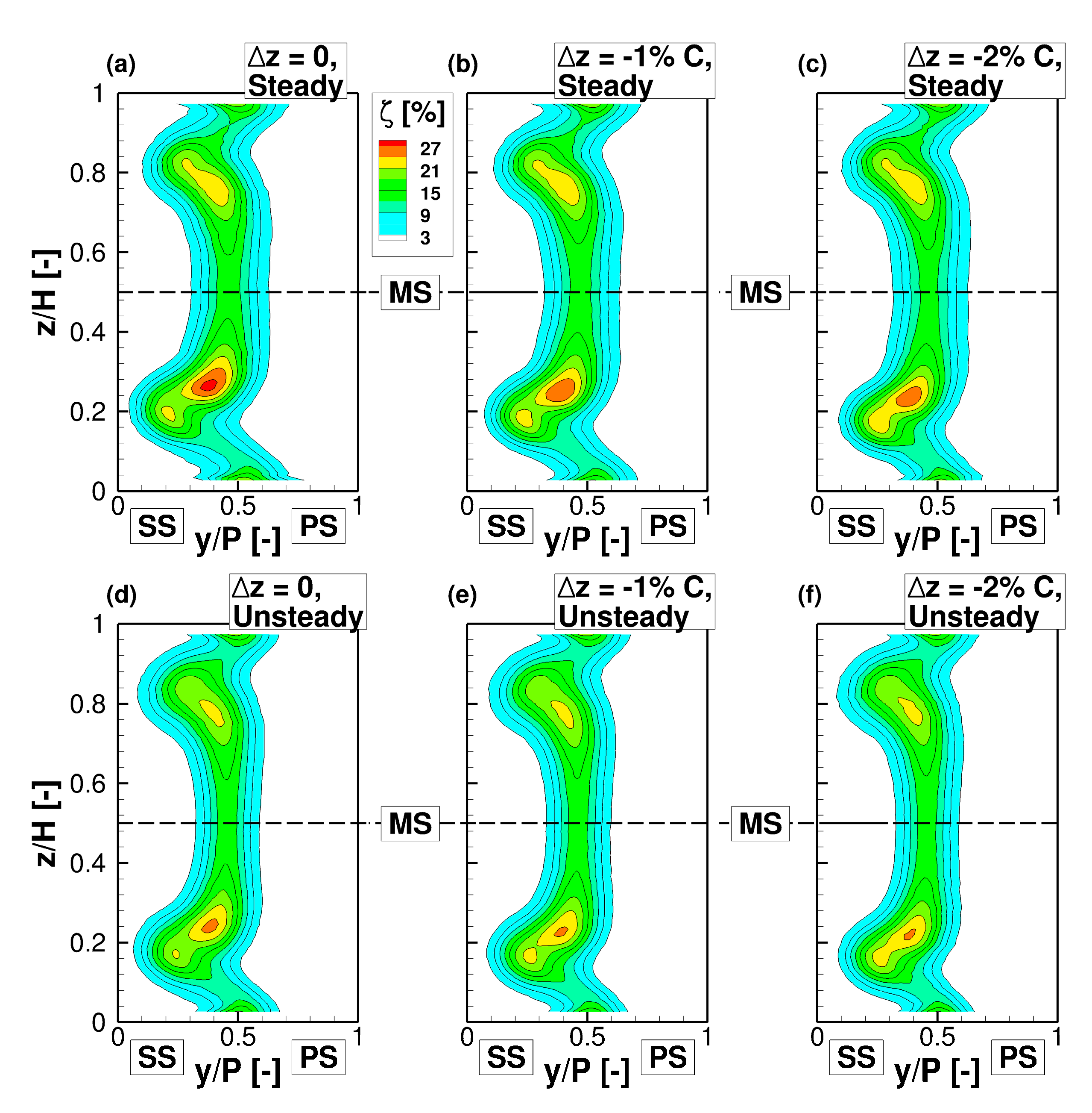
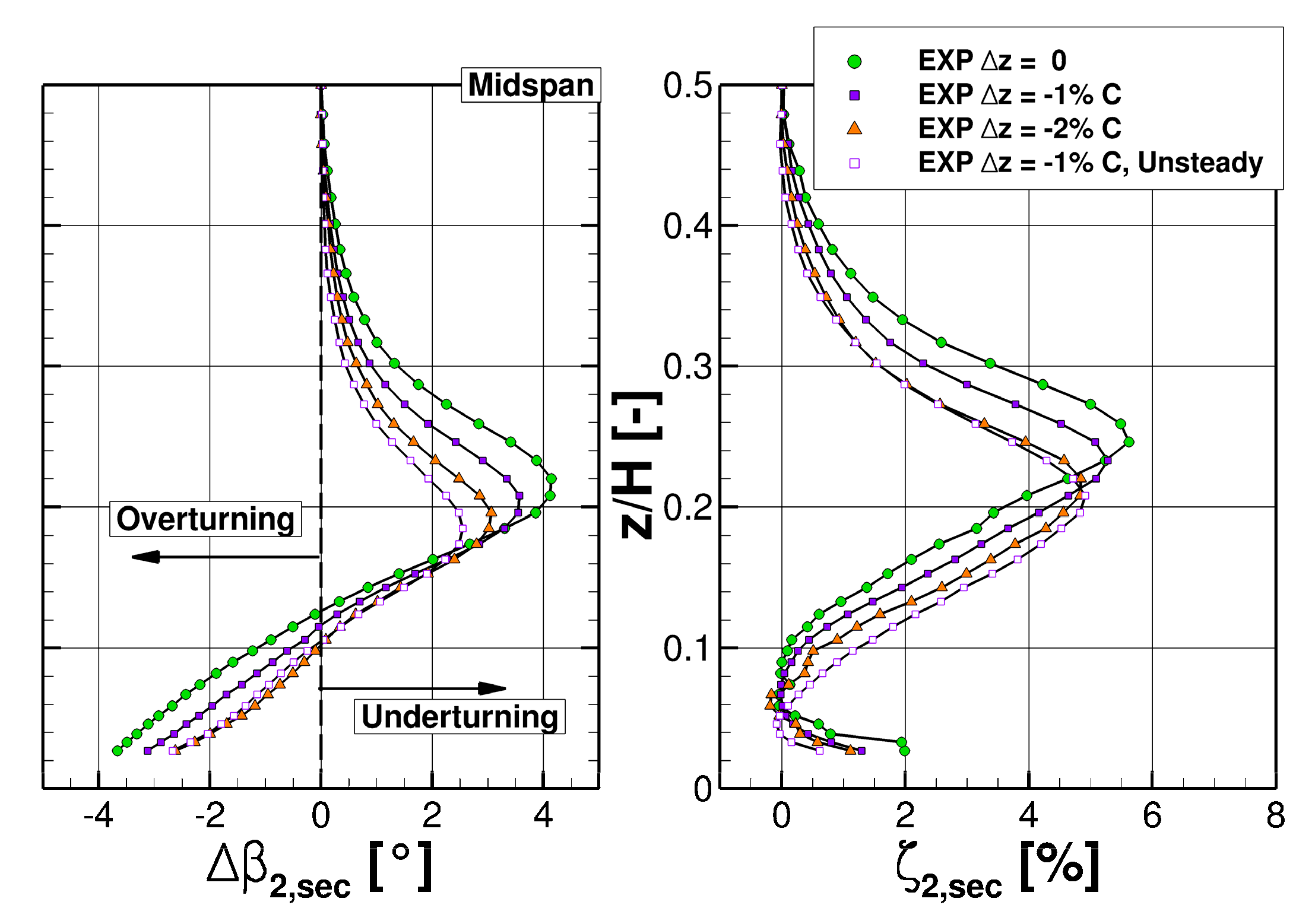
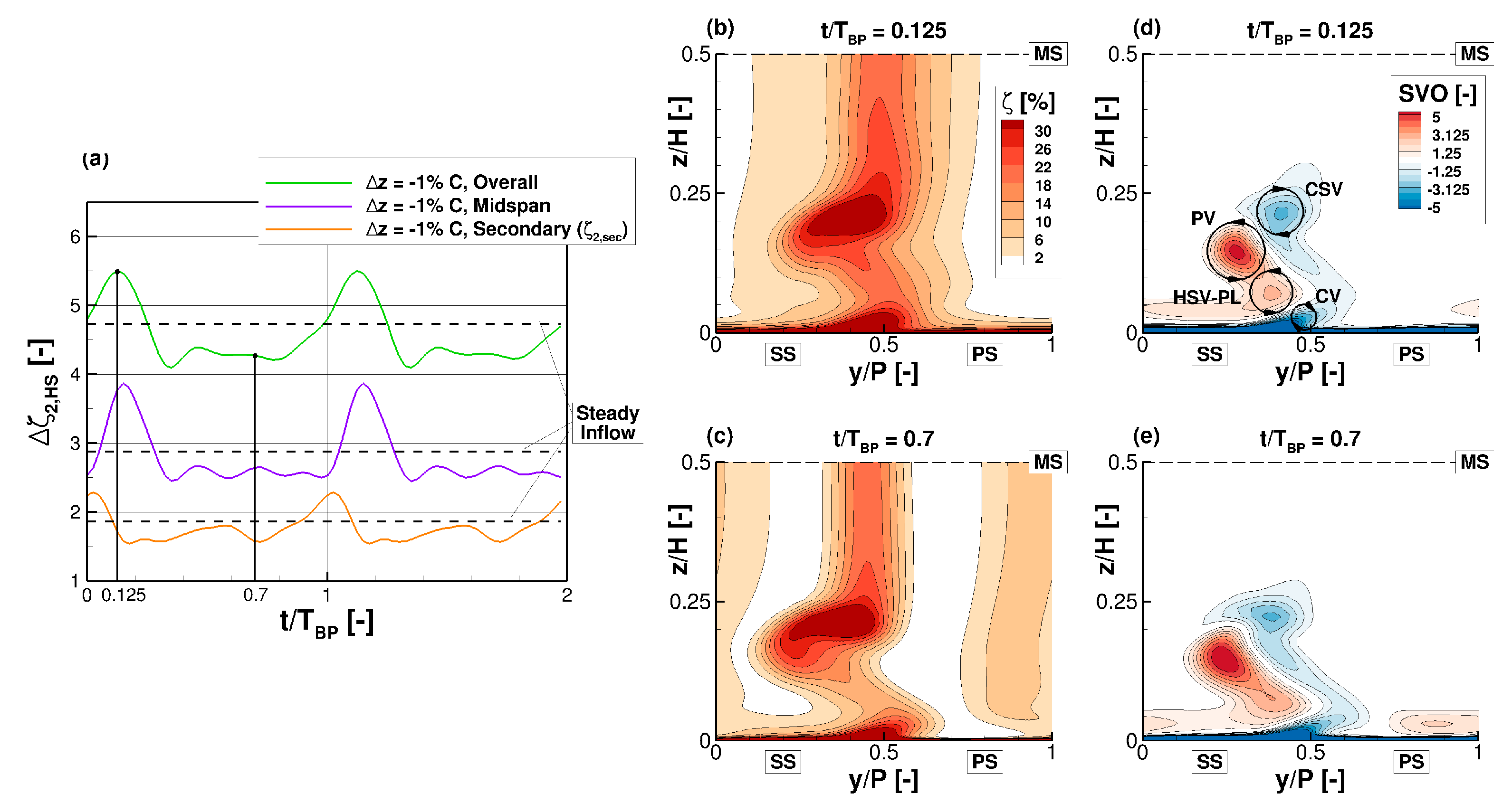
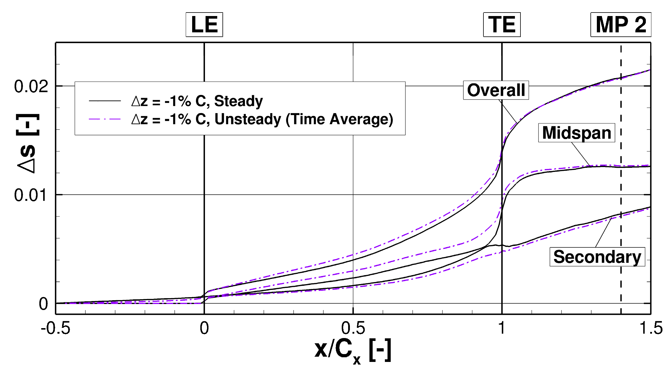
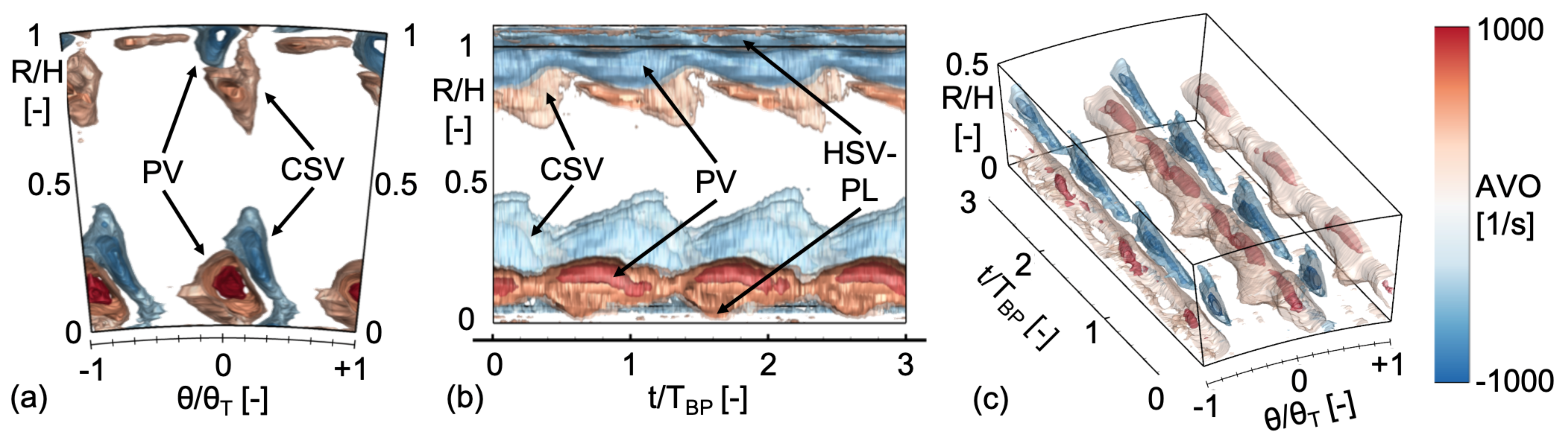
5.4.3. Impact on the Secondary Flow Structures

In this last section, the combined impact of the bar wakes and the described modified boundary layer system on the secondary flow system is portrayed on the basis of three equidistant flow field snapshots of one bar wake period in Figure 32 for Sr = 1.33, φ = 0.97. The shown quantity in the top of the figure (a) is the axial vorticity (AVO), which was derived from the spatial gradients of the time-resolved velocity vector components. The profile TEs are highlighted with dashed lines. Comparing the three AVO-distributions, both a vortex displacement as well as a weakening become evident, resulting from the wake-boundary layer interaction in the T106^RUB blade passage. Thus, especially in the hub region, a distinction between passage vortex (PV) and the pressure side leg of the horse shoe vortex (HSV-PL) is enabled for t/T_BP = 1/3, as the HSV-PL slides beneath the PV and pushes it along the suction side trailing edge radially inward, before it blends again with the PV. As could be shown in detail in [52,53,55,56], this periodic and short-duration event is based on the upstream wake impact on the developing HSV-PL, which is massively diverted in the front part of the blade passage by the impinging wake structure. Also, the unsteadiness of the suction side corner separation, shaping the concentrated shed vortex (CSV) can be realized. Additionally, in the lower half of the figure the temporal evolution of the turbulence intensity (TI) is shown. Different from the vorticity representation, the turbulence intensity not only highlights the secondary flow regions, but also emphasizes the influence of the bar wake with its increased turbulence. This becomes especially evident for t/T_BP = 2/3, when the wake becomes evident in the center of the passage between the two Tes. Even after passing through the passage, the wake still transports significant turbulence. Thus, in multistage environments, the subsequent blade row and the transition processes occurring therein are still inevitably affected.

Finally, Figure 33 is meant to clarify this vortex behavior even further by using suitable AVO iso-contours for the individual vortices and their temporal evolution.

In Figure 33a the familiar view against the axial flow direction is given, showing the colored vortices of PV and CSV, whereas Figure 33b shows this situation with the view onto the time-axis (t/T_BP), indicating the wave-like behavior of the vortex-dynamics. Furthermore, this method of data representation clearly illustrates the combination of periodic weakening and the connected displacement, defining the unsteadiness of the secondary flow system. On the one hand, the interaction mechanisms between HSV-PL and PV (periodic displacement and weakening) can be detected. On the other hand, the considerable magnitude of radial CSV-displacement resulting from HSV-PL and PV manipulation is realized. Following the short-duration weakening of PV and HSV-PL, the CSV is shifted towards the endwalls shortly after, as well. Supplementing, Figure 33c shows a three-dimensional depiction of the lower flow channel half between R/H = 0 and R/H = 0.5, thus only the near-hub part of the secondary flow system. This helps to clarify the dynamics of interaction between PV and HSV-PL, illustrating the approaching HSV-PL, its impact on the PV and the following radial PV-displacement.

5.5. Work in Progress

Upcoming activities in sub-project D include the application of particle image velocimetry (PIV) for an extended insight into the T106^RUB passage flow, the consideration of tip leakage flow, the resulting tip leakage vortices and their impact on the secondary flow system. For this, a radial gap is realized between the T106^RUB-profiles and the hub endwall contour. This increase in complexity means another step from the scientific point of view towards multistage turbomachine flow.

6. Summary and Conclusions

The current paper presents investigations of four German research institutes from a joint research project on near-wall flow in axial compressors and axial turbines. Both numerical and experimental methods were exploited on linear and annular setups to evaluate the influence of incoming periodic disturbances, which can be seen in rotor-stator-interactions, on the flow in a passage of turbomachinery. Furthermore, analyzing factors arising from the problem of transformation between a linear cascade and the rotating machine, such as the relative motion between blades/vanes and the corresponding sidewall, broadened the understanding of the secondary flow phenomena and allowed the assessment of the transferability of the obtained findings.

In sub-project A the comparison of a periodically disturbed and un-disturbed single rotor row is used to evaluate the influence of incoming wakes on the secondary flow, especially the tip leakage vortex, in the blade passage. The presented results show a redistribution of mass flow over the channel height and a periodic effect of the incoming wakes on the TLV as well as on the suction side separation. Changing the hub wall motion in a stator configuration allowed the examination of the influence of incoming boundary layer skew, the relative motion between vane tip and corresponding endwall, and a combined effect on the tip leakage vortex.

Sub-project B considered a linear compressor cascade where the investigated vane was derived from the tip profile of the rotor considered in sub-project A. Investigations were conducted using high resolving DNS and Wall-Resolving LES. In doing so, the effects of relative wall motion and thickness of the boundary layer on the vortical structures within the cascade were studied. It is clearly shown that the relative wall motion causes a departure of the tip leakage vortex from the blade profile and furthermore, a stratification of the flow field at the cascade exit.

Complementary, a linear low-pressure turbine cascade was used for high-speed wind tunnel measurements and URANS simulations in sub-project C. As the authors illustrate, a decrease of the inlet endwall boundary layer height and periodically incoming wakes both lead to secondary flow attenuation in the turbine exit flow. Inside the blade passage, the variation of inlet boundary layer thickness influences the endwall loss development starting around the midpoint of the blade passage. Furthermore, it could be shown that the unsteady inflow conditions lead to a spatial redistribution of the loss generation inside the blade passage. A premature loss increase due to wake interaction with the blade surface boundary layer is followed by attenuation of the profile- and secondary losses in the aft-section of the blade passage. However, the level of integral loss in the turbine exit flow field remains almost unchanged.

Finally, in sub-project D a large-scale annular turbine test rig was considered using modified blades of those that were studied in sub-project C. Customized surface-mounted hot-film sensor arrays were used to investigate the near-wall flow for several perturbation frequencies of upstream installed rotating bars. Thus, it was possible to discover in detail, how periodically incoming wakes lead to a recurrent cycle of formation, weakening and displacement of specific components of the underlying vortex structures as well as a periodic manipulation of the profile boundary layer system.

To sum it up, the collaborative activity of the four research institutes, presented in this publication, helps to deepen the understanding of near-wall flow, vortex systems and corresponding flow phenomena in turbomachines. The investigation of periodically distortions by incoming wakes and their interaction with the near-wall flow field in all investigated configurations (compressor and turbine, linear and annular cascades) revealed a strong influence of the wakes on the blade profile boundary layer development, especially through wake induced transition processes, while the secondary flow vortex system features a periodic displacement and changing strength. Regarding the systematic increase of complexity through the different geometric modifications and test rigs and thus activation of specific flow effects it can be concluded that the inlet boundary layer is of high relevance for the turbine endwall secondary flows, where no radial clearances are present. In a linear compressor cascade with radial clearance only the skew of the inlet boundary layer but not its thickness showed a relevant effect on the flow field. Experimental and numerical analysis in sub-project A and B clearly illustrated the effect of the relative side wall velocity on the development of the tip leakage vortex and its loss of coherence towards the exit of the blade passage. Ongoing work will apply additional measurement techniques (optical measurements, temperature sensitive paint, etc.) to provide further high-quality data for the validation of advanced numerical methods and improved physical understanding.

References

1. Von der Bank, R.; Donnerhack, S.; Rae, A.; Cazalens, M.; Lundbladh, A.; Dietz, M. LEMCOTEC: Improving the Core-Engine Thermal Efficiency. In Proceedings of the ASME Turbo Expo, Düsseldorf, Germany, 16–20 June 2014. GT2014-25040. [Google Scholar] [CrossRef]
2. ETN Global. R&D Recommendation Report 2016—For the Next Generation of Gas Turbines—Revised Edition; ETN a.i.s.b.l.: Brussels, Belgium, 2017. [Google Scholar]
3. To, H.; Miller, R. The Effect of Aspect Ratio on Compressor Performance. ASME J. Turbomach. 2019, 141, 081011. [Google Scholar] [CrossRef] [Green Version]
4. Horlock, J.H.; Lakshminarayana, B. Secondary Flows: Theory, Experiment and Application in Turbomachinery Aerodynamics. Annu. Rev. Fluid Mech. 1973, 5, 247–280. [Google Scholar] [CrossRef]
5. Peacock, R.E. A Review of Turbomachinery Tip Gap Effects: Part 1: Cascades. Int. J. Heat Fluid Flow 1982, 3, 185–193. [Google Scholar] [CrossRef]
6. Peacock, R.E. A Review of Turbomachinery Tip Gap Effects: Part 2: Rotating Machinery. Int. J. Heat Fluid Flow 1983, 4, 3–16. [Google Scholar] [CrossRef]
7. Sieverding, C.H. Recent Progress in the Understanding of Basic Aspects of Secondary Flows in Turbine Blade Passages. J. Eng. Gas Turbines Power 1985, 107, 248–257. [Google Scholar] [CrossRef]
8. Liu, Y.; Tan, L.; Wang, B. A Review of Tip Clearance in Propeller, Pump and Turbine. Energies 2018, 11, 2202. [Google Scholar] [CrossRef] [Green Version]
9. Bunker, R.S. A Review of Turbine Blade Tip Heat Transfer. Ann. N. Y. Acad. Sci. 2001, 934, 64–79. [Google Scholar] [CrossRef]
10. Langston, L.S. Secondary Flows in Axial Turbines-A Review. Ann. N. Y. Acad. Sci. 2006, 934, 11–26. [Google Scholar] [CrossRef]
11. Tyacke, J.; Vadlamani, N.R.; Trojak, W.; Watson, R.; Ma, Y.; Tucker, P.G. Turbomachinery Simulation Challenges and the Future. Prog. Aerosp. Sci. 2019, 110, 100554. [Google Scholar] [CrossRef]
12. Mailach, R.; Vogeler, K. Recent German Research on Periodical Unsteady Flow in Turbomachinery. Flow Turbul. Combust. 2009, 83, 449–484. [Google Scholar] [CrossRef]
13. Dring, R.P.; Joslyn, H.D.; Hardin, L.W.; Wagner, J.H. Turbine Rotor-Stator Interaction. ASME J. Eng. Power 1982, 104, 729–742. [Google Scholar] [CrossRef]
14. Hodson, H.P.; Howell, R.J. Bladerow Interactions, Transition, and High-Lift Aerofoils in Low-Pressure Turbines. Annu. Rev. Fluid Mech. 2005, 37, 71–98. [Google Scholar] [CrossRef]
15. Tucker, P.G. Computation of Unsteady Turbomachinery Flows: Part 1—Progress and Challenges. Prog. Aerosp. Sci. 2011, 47, 522–545. [Google Scholar] [CrossRef]
16. Mailach, R. Unsteady Flow in Turbomachinery, Habilitation, Technische Universität Dresden, Dresden, 2020; TUD Press: Dresden, Germany, 2010; ISBN 978-3-941298-92-7. [Google Scholar]
17. Pfeil, H.; Herbst, R.; Schröder, T. Investigation of the Laminar-Turbulent Transition of Boundary Layers Disturbed by Wakes. ASME J. Turbomach. 1983, 105, 130–137. [Google Scholar] [CrossRef]
18. Hilgenfeld, L.; Pfitzner, M. Unsteady Boundary Layer Development Due to Wake Passing Effects on a Highly Loaded Linear Compressor Cascade. ASME J. Turbomach. 2004, 126, 493–500. [Google Scholar] [CrossRef]
19. Ernst, M.; Michel, A.; Jeschke, P. Analysis of Rotor-Stator-Interaction and Blade-to-Blade Measurements in a Two Stage Axial Flow Compressor. ASME J. Turbomach. 2011, 133, 011027. [Google Scholar] [CrossRef]
20. Smith, N.R.; Key, N.L. A Comprehensive Investigation of Blade Row Interaction Effects on Stator Loss Utilizing Vane Clocking. ASME J. Turbomach. 2018, 140, 071004. [Google Scholar] [CrossRef]
21. Boos, P.; Möckel, H.; Henne, J.M.; Selmeier, R. Flow Measurement in a Multistage Large Scale Low Speed Axial Flow Research Compressor. In Proceedings of the ASME Int. Gas Turbine Aeroengine Congr. Exhib, Stockholm, Sweden, 2–5 June 1998. 98-GT-432. [Google Scholar]
22. Künzelmann, M.; Mailach, R.; Müller, R.; Vogeler, K. Steady and Unsteady Flow Field in a Multistage Low-Speed Axial Compressor: A Test Case. In Proceedings of the ASME Turbo Expo, Berlin, Germany, 9–13 June 2008. GT2008-50793. [Google Scholar]
23. Krug, A.; Busse, P.; Vogeler, K. Experimental investigation into the effects of the steady wake-tip clearance vortex interaction in a compressor cascade. ASME J. Turbomach. 2015, 137, 061006. [Google Scholar] [CrossRef]
24. Lange, M.; Rolfes, M.; Mailach, R.; Schrapp, H. Periodic Unsteady Tip Clearance Vortex Development in a Low-Speed Axial Research Compressor at Different Tip Clearances. ASME J. Turbomach. 2018, 140, 031005. [Google Scholar] [CrossRef]
25. Busse, P.; Krug, A.; Vogeler, K. Effects of the Steady Wake-Tip Clearance Vortex Interaction in a Compressor Cascade: Part II—Numerical Investigations. In Proceedings of the ASME Turbo Expo, Düsseldorf, Germany, 16–20 June 2014. GT2014-26121. [Google Scholar]
26. Moore, R.W., Jr.; Richardson, D.L. Skewed Boundary-Layer Flow Near the End Walls of a Compressor Cascade. Trans. ASME 1957, 79, 1789–1800. [Google Scholar]
27. Koppe, B.; Lange, M.; Mailach, R. Influence of Boundary Layer Skew on the Tip Leakage Vortex of an Axial Compressor Stator. In Proceedings of the ASME Turbo Expo, Virtual, Online, 21–25 September 2020. GT2020-15940. [Google Scholar]
28. Jeong, J.; Hussain, F. On the identification of a vortex. J. Fluid Mech. 1995, 285, 69–94. [Google Scholar] [CrossRef]
29. Hinterberger, C.; Fröhlich, J.; Rodi, W. 2D and 3D Turbulent Fluctuations in Open Channel Flow with Re τ = 590 Studied by Large Eddy Simulation. Flow Turbul. Combust. 2008, 80, 225–253. [Google Scholar] [CrossRef]
30. Koschichow, D.; Fröhlich, J.; Kirik, I.; Niehuis, R. DNS of the flow near the endwall in a linear low pressure turbine cascade with periodically passing wakes. In Proceedings of the ASME Turbo Expo, Düsseldorf, Germany, 16–20 June 2014. GT2014-25071. [Google Scholar]
31. Koschichow, D.; Fröhlich, J.; Ciorciari, R.; Niehuis, R. Analysis of the influence of periodic passing wakes on the secondary flow near the endwall of a linear LPT cascade using DNS and U-RANS. In Proceedings of the 11th European Conference on Turbomachinery Fluid Dynamics & Thermodynamics, Madrid, Spain, 23–25 March 2015. [Google Scholar]
32. Baum, O.; Koschichow, D.; Fröhlich, J. Influence of the Coriolis Force on the Flow in a Low Pressure Turbine Cascade T106. In Proceedings of the ASME Turbo Expo, Seoul, Korea, 13–17 June 2016. GT2016-57399. [Google Scholar]
33. Nicoud, F.; Ducros, F. Subgrid-Scale Stress Modelling Based on the Square of the Velocity Gradient Tensor. FlowTurbul. Combust. 1999, 62, 183–200. [Google Scholar] [CrossRef]
34. Piomelli, U.; Chasnov, J.R. Large-Eddy Simulations: Theory and Applications. In Turbulence and Transition Modelling; Hallbäck, M., Henningson, D.S., Johansson, A.V., Alfredsson, P.H., Eds.; Springer: Dordrecht, The Netherlands, 1996; pp. 269–336. [Google Scholar] [CrossRef]
35. Ventosa-Molina, J.; Lange, M.; Mailach, R.; Fröhlich, J. Study of Relative Endwall Motion Effects in a Compressor Cascade Through Direct Numerical Simulations. ASME J. Turbomach. 2021, 143, 011005. [Google Scholar] [CrossRef]
36. Michelassi, V.; Wissink, J.G.; Fröhlich, J.; Rodi, W. Large-Eddy Simulation of Flow Around Low-Pressure Turbine Blade with Incoming Wakes. Aiaa J. 2003, 41, 2143–2156. [Google Scholar] [CrossRef]
37. Inoue, M.; Kuroumaru, M. Structure of Tip Clearance Flow in an Isolated Axial Compressor Rotor. ASME J. Turbomach. 1989, 111, 250–256. [Google Scholar] [CrossRef]
38. Storer, J.; Cumpsty, N. Tip Leakage Flow in Axial Compressors. ASME J. Turbomach. 1991, 113, 252–259. [Google Scholar] [CrossRef]
39. Wissink, J.G.; Rodi, W. Numerical study of the near wake of a circular cylinder. Int. J. Heat Fluid Flow 2008, 29, 1060–1070. [Google Scholar] [CrossRef]
40. Niehuis, R.; Bitter, M. The High-Speed Cascade Wind Tunnel at the Bundeswehr University Munich after a Major Revision and Upgrade. In Proceedings of the 14th European Conference on Turbomachinery Fluid dynamics & Thermodynamics, Gdansk, Poland, 12–16 April 2021. [Google Scholar]
41. Ciorciari, R.; Kirik, I.; Niehuis, R. Effects of Unsteady Wakes on Secondary Flows in the Linear T106 Turbine Cascade. ASME J. Turbomach. 2014, 136, 091010. [Google Scholar] [CrossRef]
42. Kirik, I.; Niehuis, R. Comparing the Effect of Unsteady Wakes on Parallel and Divergent Endwalls in a LP Turbine Cascade. In Proceedings of the International Gas Turbine Congress, Tokyo, Japan, 15–20 November 2015. IGTC2015-137. [Google Scholar]
43. Kirik, I.; Niehuis, R. Experimental Investigation on Effects of Unsteady Wakes on the Secondary Flows in the Linear T106 Turbine Cascade. In Proceedings of the ASME Turbo Expo, Montreal, Canada, 15–19 June 2015. GT2015-43170. [Google Scholar]
44. Kirik, I.; Niehuis, R. Influence of Unsteady Wakes on the Secondary Flows in the Linear T106 Turbine Cascade. In Proceedings of the ASME Turbo Expo, Seoul, Korea, 13–17 June 2016. GT2016-56350. [Google Scholar]
45. Schubert, T.; Chemnitz, S.; Niehuis, R. The Effects of Inlet Boundary Layer Condition and Periodically Incoming Wakes on Secondary Flow in a Low Pressure Turbine Cascade. ASME J. Turbomach. 2021, 143, 041001. [Google Scholar] [CrossRef]
46. Wilcox, D.C. Turbulence Modeling for CFD, 4th ed.; DCW Industries: La Canada, FL, USA, 2004. [Google Scholar]
47. Langtry, R.B.; Menter, F.R. Transition Modeling for General CFD Applications in Aeronautics. In Proceedings of the 43rd AIAA Aerospace Sciences Meeting and Exhibit, Reno, NV, USA, 10–13 January 2005. AIAA 2005-522. [Google Scholar]
48. Schubert, T.; Niehuis, R. Numerical Investigation of Loss Development in a Low-Pressure Turbine Cascade with Unsteady Inflow and Varying Inlet Endwall Boundary Layer. In Proceedings of the ASME Turbo Expo, Virtual, Online, 7–11 June 2021. GT2021-59696, to be published. [Google Scholar]
49. Ciorciari, R.; Schubert, T.; Niehuis, R. Numerical Investigation of Secondary Flow and Loss Development in a Low Pressure Turbine Cascade with Divergent Endwalls. Int. J. Turbomach. Propuls. Power 2018, 3, 5. [Google Scholar] [CrossRef] [Green Version]
50. Mayle, R. The 1991 IGTI Scholar Lecture: The Role of Laminar-Turbulent Transition in Gas Turbine Engines. ASME J. Turbomach. 1991, 113, 509–536. [Google Scholar] [CrossRef]
51. Sinkwitz, M.; Engelmann, D.; Mailach, R. Experimental investigation of periodically unsteady wake impact on the secondary flow in a 1.5 stage full annular LPT cascade with modified T106 blading. In Proceedings of the ASME Turbo Expo, Charlotte, NC, USA, 26–30 June 2017. GT2017-64390. [Google Scholar]
52. Sinkwitz, M.; Winhart, B.; Engelmann, D.; di Mare, F.; Mailach, R. Experimental and Numerical Investigation of Secondary Flow Structures in an Annular LPT Cascade under Periodic Wake Impact–Part 1: Experimental Results. ASME J. Turbomach. 2019, 141, 021008. [Google Scholar] [CrossRef]
53. Sinkwitz, M.; Winhart, B.; Engelmann, D.; di Mare, F.; Mailach, R. On the Periodically Unsteady Interaction of Wakes, Secondary Flow Development, and Boundary Layer Flow in An Annular Low-Pressure Turbine Cascade: An Experimental Investigation. ASME J. Turbomach. 2019, 141, 091001. [Google Scholar] [CrossRef]
54. Sinkwitz, M.; Winhart, B.; Engelmann, D.; di Mare, F. Time-Resolved Measurements of the Unsteady Boundary Layer in an Annular Low-Pressure Turbine Configuration with Perturbed Inlet. In Proceedings of the ASME Turbo Expo, Virtual, Online, 21–25 September 2020. GT2020-15319. [Google Scholar]
55. Winhart, B.; Sinkwitz, M.; Engelmann, D.; di Mare, F.; Mailach, R. On the Periodically Unsteady Interaction of Wakes, Secondary Flow Development and Boundary Layer Flow in an Annular LPT Cascade. Part 2–Numerical Investigation. In Proceedings of the ASME Turbo Expo, Oslo, Norway, 11–15 June 2018. GT2020-76873. [Google Scholar]
56. Winhart, B.; Sinkwitz, M.; Schramm, A.; Engelmann, D.; di Mare, F.; Mailach, R. Experimental and Numerical Investigation of Secondary Flow Structures in an Annular LPT Cascade under Periodic Wake Impact–Part 2: Numerical Results. ASME J. Turbomach. 2019, 141, 021009. [Google Scholar] [CrossRef] [Green Version]
57. Winhart, B.; Sinkwitz, M.; Schramm, A.; Post, P.; di Mare, F. Large-Eddy Simulation of Periodic Wake Impact on Boundary Layer Transition Mechanisms on a Highly Loaded Low-Pressure Turbine Blade. In Proceedings of the ASME Turbo Expo, Virtual, Online, 21–25 September 2020. GT2020-14555. [Google Scholar]
58. Sinkwitz, M. Experimentelle Untersuchung der Entstehung von Sekundärstömung in Turbinen-Ringgittern unter Periodisch-Instationärer Zuströmung. Ph.D. Thesis, Ruhr-Universität Bochum, Universitätsbibliothek, Bochum, Germany, 2021. [Google Scholar] [CrossRef]
59. Hodson, H.P.; Howell, R.J. The Role of Transition in High-Lift Low-Pressure Turbines for Aeroengines. Prog. Aerosp. Sci. 2005, 41, 419–454. [Google Scholar] [CrossRef]
60. Stieger, R.D.; Hodson, H.P. The Transition Mechanism of Highly Loaded Low-Pressure Turbine Blades. ASME J. Turbomach. 2004, 126, 536–543. [Google Scholar] [CrossRef]
61. Hodson, H.P.; Huntsman, I.; Steele, A.B. An Investigation of Boundary Layer Development in a Multistage LP Turbine. ASME J. Turbomach. 1994, 116, 375–383. [Google Scholar] [CrossRef]
62. Halstead, D.E.; Wisler, D.C.; Okiishi, T.H.; Walker, G.J.; Hodson, H.P.; Shin, H.-W. Boundary Layer Development in Axial Compressors and Turbines: Part 1 of 4—Composite Picture. ASME J. Turbomach. 1997, 119, 114–127. [Google Scholar] [CrossRef]
63. Mahallati, A.; Sjolander, S.A. Aerodynamics of a Low-Pressure Turbine Airfoil at Low-Reynolds Numbers -Part II: Blade-Wake Interaction. ASME J. Turbomach. 2013, 135, 011011. [Google Scholar] [CrossRef]
Figure 1. Low Speed Research Compressor (LSRC)—cross section of investigated setups with stator S1 (a) and rotor R1 (b).
Ijtpp 06 00009 g001
Figure 2. Pitchwise averaged total pressure pt (black) and flow angle α (orange) upstream of S1 (MP4) in the hub endwall region, s/C = 2.0%, EXP vs. CFD.
Ijtpp 06 00009 g002
Figure 3. Effect of varying hub wall motion on non-dimensional total pressure loss coefficient downstream of S1 (MP5) (ac) EXP, (dg) CFD, and on the TLV trajectory ( λ 2 ( v ) = 10 6 ) (hk) CFD, s/C = 2.0%.
Ijtpp 06 00009 g003
Figure 4. Effect of varying hub wall motion on pitchwise averaged flow angle in absolute frame of reference downstream of S1 (MP5), s/C = 2.0%, CFD.
Ijtpp 06 00009 g004
Figure 5. Effect of incoming periodic transient wakes on (a) time- and pitchwise averaged data up- (MP3) and downstream (MP4) of R1, (b) ensemble- and pitchwise averaged FMP data and (c) ensemble averaged FMP data at discrete relative positions between WG and R1 downstream of R1 (MP4), s/C= 1.36%, EXP.
Ijtpp 06 00009 g005
Figure 6. Top down view of the simulated linear cascade profile with zoom of the computational domain (shaded region), repeated in y-direction (grey). Coordinates are scaled using the blade chord. Red dashed line at x / C = 0.89 depicts the stage outlet plane.
Ijtpp 06 00009 g006
Figure 7. Linear compressor cascade at Re C = 1.46 10 4 . (a) Vortical structure visualized through λ 2 ( v ) = 2 . (b) Pitchwise averaged total pressure losses downstream of the blade at x / C = 0.89 .
Ijtpp 06 00009 g007
Figure 8. Comparison of WRLES and DNS results along the blade at different spanwise positions. (a) Friction c f along the SS and (b) pressure c p along PS and SS.
Ijtpp 06 00009 g008
Figure 9. Time averaged pressure coefficient at the endwall ( z = 0 ). Results from (a) WRLES and (b) experiments [23].
Ijtpp 06 00009 g009
Figure 10. Pitchwise averaged (a) total pressure losses ζ and (b) flow angle deviation Δ β 2 , downstream of the blade (plane at x / C = 0.89 ). Experimental data from Krug et al. [23].
Ijtpp 06 00009 g010
Figure 11. Vortical structure ( λ 2 ( v ) = 2 ) for the linear compressor cascade at Re c = 3 10 5 .
Ijtpp 06 00009 g011
Figure 12. Pressure (a) and friction (b) coefficients on the blade at two different spanwise positions, near the blade tip ( z / H = 0.06 ) and at midspan ( z / H = 0.3 ).
Ijtpp 06 00009 g012
Figure 13. Blade suction side boundary layer state, characterized through the turbulent kinetic energy (TKE) in normal direction to the blade ( η / C ) and the shape factor ( H 12 ).
Ijtpp 06 00009 g013
Figure 14. Cutplanes downstream of the blade (plane at x / C = 0.89 ) of (a) total pressure losses and (b) TKE. Pitchwise coordinate normalized by cascade pitch P with origin such that the wake is located at the centre, PS on the left.
Ijtpp 06 00009 g014
Figure 15. Vortical structure ( λ 2 ( v ) = 2 ) for the linear compressor cascade at Re c = 3 10 5 with relative motion between blade and endwall. Black lines with arrows at the bottom denote the endwall motion.
Ijtpp 06 00009 g015
Figure 16. Effect of relative motion downstream of the blade (plane at x / C = 0.89 ). Cutplane of (a) total pressure and (b) TKE. In these two figures, the pitch is normalized by cascade pitch P and its origin such that the wake appears in the centre. (c) Pitchwise averaged total pressure losses. Experimental data from Krug et al. [23].
Ijtpp 06 00009 g016
Figure 17. Effect of incoming wakes on blade performance characteristics at the suction side near the blade tip ( z / H = 0.06 ) and in the midspan region ( z / H = 0.30 ). (a) Time averaged pressure coefficient (Equation 3) with shaded areas denoting the span of transient fluctuations. (b,c) Friction coefficient ( c f ) near the blade tip and in the midspan region, respectively.
Ijtpp 06 00009 g017
Figure 18. Effect of the flat plate misalignment on the inlet endwall boundary layer of the T106A cascade.
Ijtpp 06 00009 g018
Figure 19. Block topology in the computational domain of the T106A cascade with an integrated two-part flat plate and a moving bar wake generator.
Ijtpp 06 00009 g019
Figure 20. Comparison of the predicted and measured isentropic Mach number distributions at midspan of the T106A turbine cascade at M exit , th = 0.59 ,   Re exit , th = 2 · 10 5 .
Ijtpp 06 00009 g020
Figure 21. Measured total pressure losses at different endwall boundary layer conditions, (ac) with and (df) without periodically incoming wakes in MP2.
Ijtpp 06 00009 g021
Figure 22. Measured spanwise distributions of the pitchwise-averaged secondary pitch angle Δ β 2 ,   sec and secondary total pressure losses ζ 2 ,   sec under different endwall boundary layer conditions, with and without periodically incoming wakes in MP2.
Ijtpp 06 00009 g022
Figure 23. Numerical prediction of the change in (a) integral- and (b,c) local total pressure losses as well as (d,e) streamwise vorticity over time in MP2 with unsteady inflow conditions.
Ijtpp 06 00009 g023
Figure 24. Axial entropy development throughout the T106A blade passage with steady and unsteady inflow conditions.
Ijtpp 06 00009 g024
Figure 25. Test facility Axial Turbine II: sectional view (a), 3D illustration (b).
Ijtpp 06 00009 g025
Figure 26. Selected devices for the acquisition of time-resolved measurement data: Dantec Dynamics type 55R56 and 55R57 SFP (a), assembly of modular T106RUB blade with suction side hot-film instrumentation (b), arrangement of Kulite LQ-125 sensors along the profile (c).
Ijtpp 06 00009 g026
Figure 27. Time-resolved flow field quantities downstream of the rotating wake generator: velocity v (a), flow angle in circumferential direction α (b) and turbulence intensity TI (c) over channel height R/H for Sr = 1.33, φ = 0.97.
Ijtpp 06 00009 g027
Figure 28. Time-averaged distributions of velocity v (a), flow angle in circumferential direction α (b) and turbulence intensity TI (c) over channel height R/H downstream of the rotating wake generator for Sr = 1.33, φ = 0.97 and clean inflow, see [58].
Ijtpp 06 00009 g028
Figure 29. cp distributions for clean and perturbed inflow at T106RUB midspan, time-averaged results (a), superposition of maximal fluctuation values (b), see [58].
Ijtpp 06 00009 g029
Figure 30. Temporal evolution of pressure fluctuations along the T106RUB profile at midspan for Sr = 0.43 (a), Sr = 0.90 (b) and Sr = 1.33 (c), see [58].
Ijtpp 06 00009 g030
Figure 31. Temporal evolution of QWSS along the T106RUB profile suction side at midspan for Sr = 0.43 (a) and Sr = 1.33 (b), undisturbed condition shown above, see [58].
Ijtpp 06 00009 g031
Figure 32. Temporal flow field evolution in the T106RUB exit flow field (Δx = 0.16 C) at 3 equidistant time steps, Sr = 1.33, φ = 0.97. Axial vorticity (AVO) (a) and turbulence intensity (TI) (b).
Ijtpp 06 00009 g032
Figure 33. Temporal AVO flow field evolution (iso-contours) in the T106RUB exit flow field (Δx = 0.16 C) with the time as the third dimension, Sr = 1.33, φ = 0.97. View of radial-circumferential plane (a), of radial-axial plane (b) and of the lower half of the secondary flow system in a three-dimensional depiction (c), see [58].
Ijtpp 06 00009 g033