Hybrid Data-Driven and Physics-Based Modeling for Gas Turbine Prescriptive Analytics

Abstract

This paper presents a methodology for predictive and prescriptive analytics of a gas turbine. The methodology is based on a combination of physics-based and data-driven modeling using machine learning techniques. Combining these approaches results in a set of reliable, fast, and continuously updating models for prescriptive analytics. The methodology is demonstrated with a case study of a jet-engine power plant preventive maintenance and diagnosis of its flame tube. The developed approach allows not just to analyze and predict some problems in the combustion chamber, but also to identify a particular flame tube to be repaired or replaced and plan maintenance actions in advance.

1. Introduction

Following Gartner [1], prescriptive analytics is a form of advanced analytics which examines data or content to answer the question “What should be done?”. In structural health monitoring and industrial asset management, it is used to build solutions aiming to prescribe particular actions in order to avoid malfunctions and defects development during machine operation. This methodology is of high interest in the engineering community [2,3,4] since it can be considered as the next step towards predictive analytics and it leads to optimized decision making.

For predictive analytics of gas turbines, a physics-based approach and a data-driven approach are the two most common methods. Prescriptive analytics requires a combination of both approaches together with digital twin technology, as it is shown hereafter.

1.1. Physics-Based Approach

The physics-driven approach uses numerical modeling of a gas turbine and its subsystems. Gas turbines’ working processes are described mostly by thermodynamics equations. Modeling includes computational fluid dynamics (CFD) simulation of compressors and turbines [5], simulation of the burning process [6], and high-level modeling [7]. Typically, a physical model is designed using a combination of disciplines, such as hydraulics, pneumatics, mechanics, electromechanics, thermodynamics, and chemistry. The physical model can be validated using field data.

Previous papers have presented generalized models for steady-state condition monitoring [8]. Algorithms based on exergetic analysis have shown a good correlation with the field data. The models presented in [8] can be used to determine thermodynamic parameters providing suitable operating conditions.

However, physics-based modeling also has drawbacks:

• Subsystems designed with simplified differential equations are not accurate enough for realistic simulation of a system’s dynamics. For instant, control systems can use a simplified dynamic model of the engines, but these models usually can not describe abnormal behavior, which corresponds to some developing malfunctions.
• Usually, operators and predictive system developers do not have subsystems and component characteristics (e.g., performance maps of compressors and turbines) required for physics-based model development.

1.2. Data-Driven Approach

A data-driven approach uses field data to design statistics-based or machine learning-based models. Compared with physics-based modeling, the data-driven approach does not need engineering documentation (performance maps, etc.) to develop a model. However, this approach requires a lot of field data. Algorithms such as support vector machines (SVM) have shown good results in [9,10]. SVM has been used for gas turbine fault detection, where it showed an accuracy greater than 80% for test data and gas turbine prognostics. To monitor vibration levels, algorithms such as random forest or gradient boosting are used [11]. The main problem of the implementation of these algorithms is the lack of field data for training.

Artificial neural networks (ANNs) are promising algorithms in industrial predictive analytics. An interesting application of neural networks to gas turbines is unsupervised learning [12]. This study examined the problem of gas turbine combustion monitoring. The performance of an unsupervised model was better than that of a model with handcrafted features.

The drawback of fault detection is that it does not determine the reason for the abnormal behavior it detects. This problem can deal with a model which implements explainable AI. The model does not just identify abnormal behavior of the gas turbine or other equipment, but also identifies the reason for such behavior. Moreover, lack of labeled data, which are a group of samples that have been tagged with one or more labels like different faults, complicates the development of feasible algorithms.

The complexity of the task makes it difficult to develop a model using only one of these approaches; the task requires more complicated hybrid modeling, which uses both physics-based and data-driven approaches.

1.3. Digital Twin

Traditionally, computer-aided engineering (CAE) systems and tools have focused on the development and production stages of the product life cycle, including design, testing, model validation, and manufacturing. Since the 1980s, a huge amount of data has been generated, and it is used to develop and manufacture complex products in industries such as aerospace, automotive, and machinery. Nowadays, more and more attention is paid to multi-level simulation of products to support their development process and reduce the number of physical tests needed.

System models built using systems modeling languages (SysML), functional models built in Modelica-oriented environments, finite-element models, and finite-volume models are managed using special modules in product life cycle management (PLM) systems called simulation process and data management (SPDM) modules. All the models mentioned above, along with increasing computing power, make it possible to introduce the concept of digital twins [13]. A digital twin is based on the virtual physics-driven model of a product, system, or process. The digital twin enables real-time monitoring to avoid malfunctions before they occur in its physical counterpart [14]. In addition, a digital twin reduces the cost of system testing and verification. Unlike an ordinary virtual model, which simulates a perfect product, a digital twin represents a particular instance of a product at different stages of its life cycle (testing, production, maintenance, and disposal).

In this study, we aim to utilize the concepts of digital twins and hybrid modeling for prescriptive analytics of a gas turbine engine. The efficacy of the approach will be demonstrated with a case study.

2. Materials and Methods

The study considers prescriptive analytics of an FT8 gas turbine. It is derived from the Pratt & Whitney JT8D series aircraft engine [15]. The JT8D is a two-spool engine with a fan at the compressor inlet. The configuration of the FT8 includes two new compressor stages instead of the fan. The FT8 has a turbo-annular combustor arrangement. The combustor consists of 9 individual flame tubes [16]. A high-pressure turbine (HPT), a low-pressure turbine (LPT), and a power turbine (PT) are placed after the combustion chamber. Figure 1 shows the scheme of the FT8 gas turbine.

2.1. Problem Statement

The combustion system is a critical part of any gas engine. Combustion conditions are commonly monitored in the industry [12,17]. A combustion process occurs under high pressure, temperature, and gas flow rate conditions that create high thermodynamic loading for the combustor components. Combustion instabilities and injector malfunctions may lead to imbalanced fuel distribution in the flame tubes and cause serious faults, such as fuel nozzle faults, flame tube burnouts, and intensive vibrations. These anomalies may lead to catastrophic failures of gas turbines. Thus, early detection of abnormal behaviors and flame tube malfunctions is important during the gas turbine life cycle. The flame tube malfunction can be detected based on the temperature profile of thermocouples placed at a certain distance from the combustion chamber. The FT8 gas turbine is equipped with probes which measure exhaust gas temperature (EGT). They enable operators to ensure an even temperature distribution. The system for EGT measurements consists of nine thermocouples located after the LPT (Figure 2a). Due to swirl of the exhaust gas after the combustion chamber, the thermocouple number corresponds to previous number of flame tube (for instance, the 7th thermocouple shows temperature after the 6th flame tube). In our experiments, we have done a correction on the thermocouple numbers to make it the same as the flame tube number. As a result of the EGT probes’ locations, a properly performing gas engine has a characteristic curved EGT profile. The profile has a special shape, as shown in Figure 2b. The following counting of thermocouple numbers is chosen from operation documentation. It has the best view for operators to observe possible faults.

In our work, the following data were available:

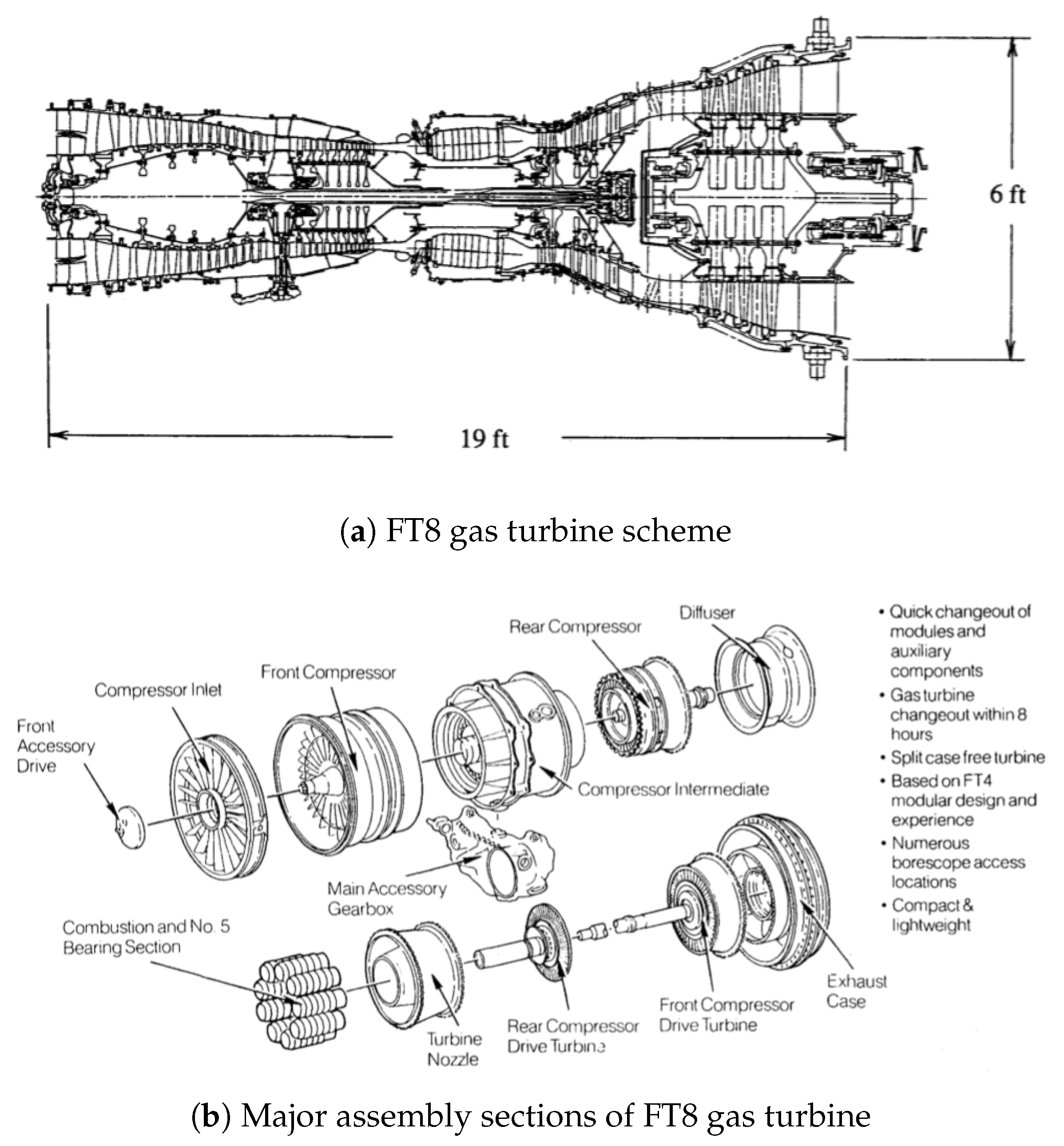
• Two years of real FT8 gas turbine field data;
• 24 features, such as pressures and temperatures in different parts of the turbine, environment conditions, shafts’ rotary speed.;
• moments of time when flame tubes were repaired;
• numbers of flame tubes which were broken.

2.2. Physics-Based Model of a Gas Turbine

In this chapter, the development of a gas turbine physics-based model is described. Gas turbine power plants produce mechanical power from the expansion of hot gases in a turbine. The Brayton cycle is a thermodynamics cycle upon which all gas turbines operate [18]. A typical industrial gas turbine power plant has two shafts and a detached power turbine, which is connected to a generator [16,19].

The physics-based model of a gas turbine enables the detection of malfunctions even without any field data, using thermodynamic laws and equations [20]. A digital twin of a gas turbine power plant would allow the operators to simulate any malfunction to perform prescriptive maintenance of gas turbines. However, the lack of data on the physical characteristics of gas turbines complicates the task of developing the digital twin of a gas turbine power plant.

Much information about FT8 gas turbine power plants required for developing a digital twin is unknown. Some papers describe an approach for the analysis of FT8 gas turbines [21,22], but this analysis is not enough to develop a digital twin.

A scaling procedure for performance maps is a helpful tool for the analysis of compressors and turbines [23]. The scaling procedure described in the present article suggests the following approach:

• An engineer defines a type of the considered compressor or turbine.
• A component of the same type with a known performance map (reference map) is taken.
• The reference map is scaled by mass flow rate, pressure ratio, rotary speed, and isentropic efficiency factors to obtain an actual performance map.

Taking into account reference maps for components of different types [5,24,25,26,27,28] makes it possible to design a physics-based model of the FT8 gas turbine.

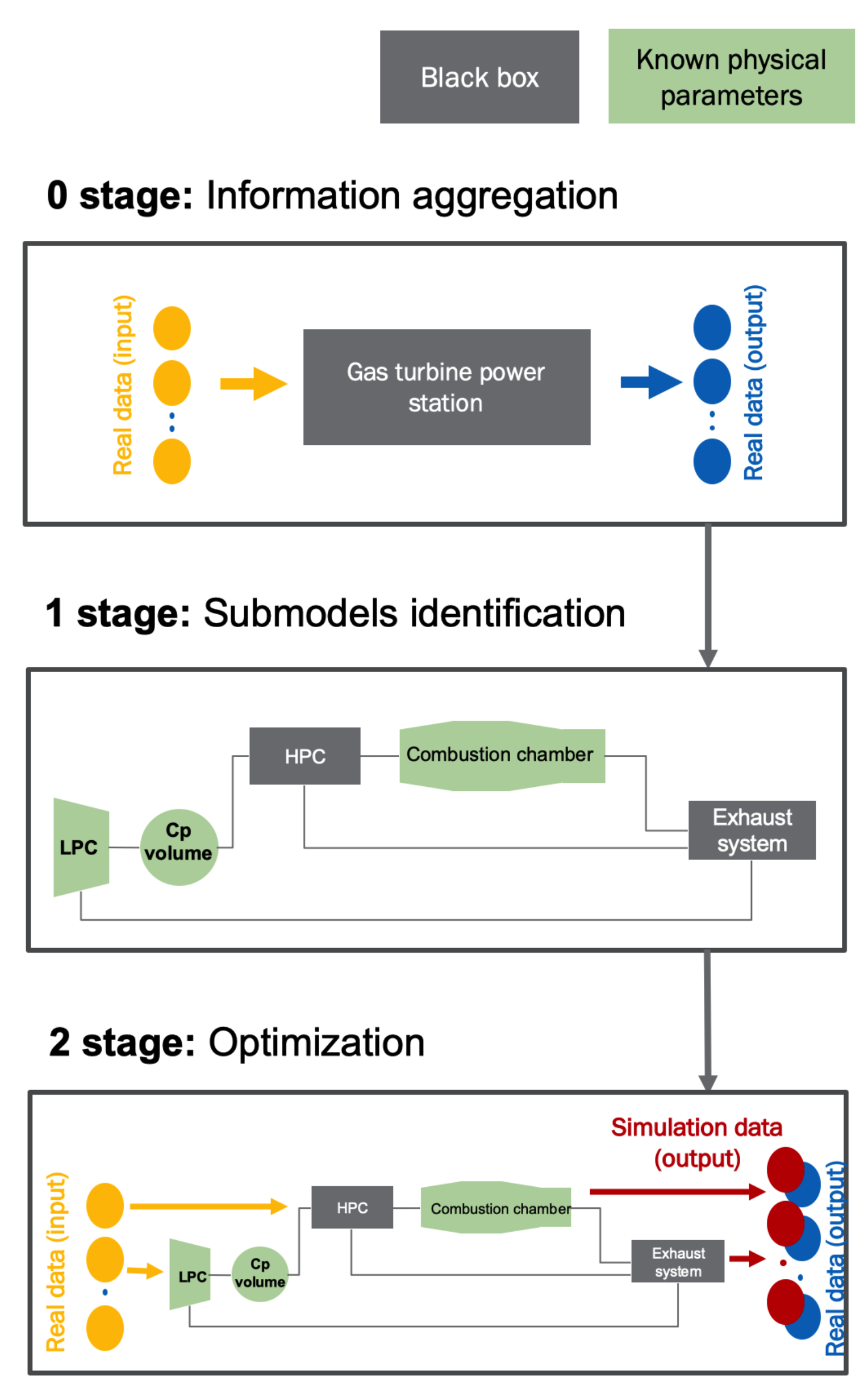
2.3. Workflow for Physical Model Development

The physics-based model was developed using the Python programming language. The model considers only a gas engine without a power turbine so it uses LPT exit conditions for simulation. The model could also be simplified assuming that the steady-state relationship of the pressure after low-pressure compressor (LPT) vs. the rotary speed of high-pressure compressor (HPC) could be defined. Figure 3 presents a workflow for the physics-based model development.

The approach used in this study consisted of three main steps:

• The model is represented as a black box. Only the input parameters and output parameters are known. The field data and model documentation are collected.
• Some subsystems are identified using papers, documentation, and measurements, while subsystems remain as black boxes.
• Optimization algorithms are used to tune the parameters of unknown subsystems using field data.

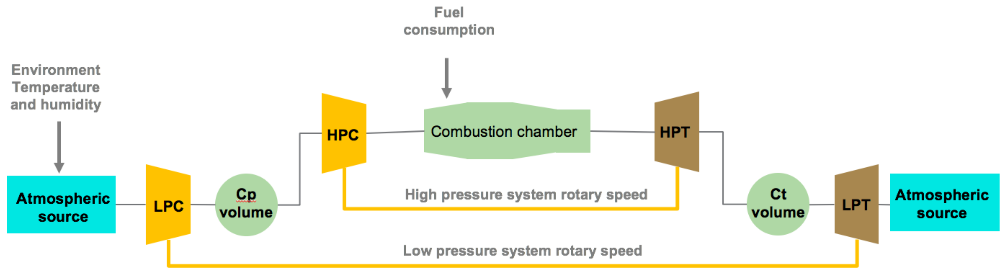
2.3.1. Subsystems Description

In this study, the physics-based model of a gas turbine was divided into submodels connected in series. The submodels were described by equations determining how they work. The model developed in this study used a gas model with a 6 component gas:

$$\overline{y}=\left(y_i\right)=\left(\begin{array}{cccccc}{N}_2& O_2& Ar& H_{2}O& C{O}_2& C_{10}{H}_{20}\end{array}\right)$$

(1)

Enthalpy of formation of species $h_{f{0}_i}$ and specific heat $c_{p_i},c_{v_i}$ vs. temperature in the range of 200 K to 6000 K were taken from NASA documentation [29]. Figure 4 represents the composition of the physical model.

The model uses field data to define initial conditions, such as the pressure in chambers, environmental temperature, pressure, and humidity. The submodels are elaborated below.

2.3.2. Atmospheric Source

The atmospheric source represents a submodel with no input and constant thermodynamic values. To be initialized, the model required pressure P, temperature T, species fraction y, and molar mass $\mu$. The submodel calculates a specific enthalpy $h_{out}$ and a heat capacity ratio $\gamma$:

$$c_{p_{mix}}\left(T\right)=\sum _{i=1}^6{y}_i{c}_{p_i}\left(T\right),c_{v_{mix}}\left(T\right)=\sum _{i=1}^6{y}_i{c}_{v_i}\left(T\right)$$

(2)

$$\gamma =\frac{c_{p_{mix}}}{c_{v_{mix}}}$$

(3)

$$h_{out}=c_{p_{mix}}T$$

(4)

2.3.3. Chamber with Constant Volume

The chamber model solves the variation of internal energy using the first law of thermodynamics for an open system. This study assumed that thermal losses due to irradiation, convection, and conductivity are negligible. To be initialized, the model requires the values of pressure P, a temperature T, species fraction y, molar mass $\mu$, and volume V. The submodel calculates the specific universal gas constant for the mixture.

$$r_{mix}=\sum _{i=1}^n\frac{y_i}{{\mu }_i}R$$

(5)

$${\rho }_{mi{x}_{init}}=\frac{P_{init}}{r_{mix}{T}_{init}}$$

(6)

$${\rho }_i=y_i{\rho }_{mix}$$

(7)

The following equations are used to calculate a steady-state condition during simulation:

$$\frac{d{\rho }_i}{dt}=\frac{1}{V}\left(y_{i_{in}}{\dot{m}}_{in}-y_{i_{out}}{\dot{m}}_{out}\right)$$

(8)

$$\frac{dT}{dt}=\frac{{\dot{m}}_{in}{h}_{in}-{\dot{m}}_{out}{h}_{out}-m{\sum }_{i=1}^6\frac{d{y}_i}{dt}{u}_i-\frac{dm}{dt}\int {}^{}{c}_{v_{mix}}dT}{m{c}_{v_{mix}}}$$

(9)

$$P={\rho }_{mix}{r}_{mix}T$$

(10)

$$h_{out}=c_{p_{mix}}\left(T\right)T$$

(11)

For fuel specific heat calculations, we use averaged value obtained with temperature on the current and previous integration steps. It can be done because of the errors of the sensors (fuel consumption sensor, temperature sensors, etc.) are higher then the integration error.

2.3.4. Compressor

A compressor performance map is the most important data for submodel initialization. The performance map defines several steady-state compressor operating regimes with interpolation for other regimes. The model also requires the values input and output pressure $P_{in}$ and $P_{out}$, input temperature $T_{in}$, and rotary speed $\omega$ to be initialized. The performance map is represented as two functions $P{M}_m(\omega ,\frac{P_{out}}{P_{in}})$ and $P{M}_{\eta }(\omega ,\frac{P_{out}}{P_{in}})$, which define mass flow rate $\dot{m}$ and isentropic efficiency $\eta$ with a correction to a real compressor’s working conditions:

$${\omega }_{corrected}={\omega }_{actual}\sqrt{\frac{290}{T_{in}}}$$

(12)

$${\dot{m}}_{corrected}=P{M}_m({\omega }_{corrected},\frac{P_{out}}{P_{in}}),\eta =P{M}_{\eta }({\omega }_{corrected},\frac{P_{out}}{P_{in}})$$

(13)

$${\dot{m}}_{actual}={\dot{m}}_{corrected}\sqrt{\frac{290}{T_{in}}}{P}_{in}$$

(14)

The outlet temperature and enthalpy are then computed:

$$T_{out}=T_{in}\left[1+\frac{{(\frac{P_{out}}{P_{in}})}^{\frac{\gamma -1}{\gamma }}-1}{\eta }\right]$$

(15)

$$h_{out}=c_{p_{mix}}\left(T\right)T$$

(16)

2.3.5. Combustion Chamber

The combustion chamber was described using the same equations as the Chamber with constant volume with some additional heat generated due to chemical reaction:

$$15O_2+C_{10}{H}_{20}\Rightarrow 10H_{2}O+10C{O}_2$$

(17)

The generated heat flow was calculated using the enthalpy of formation of species i:

$$Q_{react}=\sum {}^{}-d{m}_i{h}_{f{0}_i}$$

(18)

To calculate a steady-state condition, the thermodynamic equations from Chamber had to be changed:

$$\frac{d{\rho }_i}{dt}=\frac{1}{V}\left(y_{i_{in}}{\dot{m}}_{in}+y_{fuel}{\dot{m}}_{fuel}-y_{i_{out}}{\dot{m}}_{out}\right)$$

(19)

$$\frac{dT}{dt}=\frac{{\dot{m}}_{in}{h}_{in}+{\dot{m}}_{fuel}{h}_{fuel}-{\dot{m}}_{out}{h}_{out}+\frac{d{Q}_{react}}{dt}-m{\sum }_{i=1}^6\frac{d{y}_i}{dt}{u}_i-\frac{dm}{dt}\int {}^{}{c}_{v_{mix}}dT}{m{c}_{v_{mix}}}$$

(20)

$$P={\rho }_{mix}{r}_{mix}T$$

(21)

$$h_{out}=c_{p_{mix}}\left(T\right)T$$

(22)

2.3.6. Turbine

The turbine submodel had the same initialization requirements, inputs, and outputs as the Compressor submodel, but the outlet temperature was calculated in a different way:

$$T_{out}=T_{in}\left[1+({(\frac{P_{out}}{P_{in}})}^{\frac{\gamma -1}{\gamma }}-1)\eta \right]$$

(23)

where $\eta$ is the isentropic efficiency of a turbine. Mass flow rate $\dot{m}$ and isentropic efficiency $\eta$ were determined by the performance map of a turbine. Mass flow rate and rotary speed were corrected as described in the Compressor model.

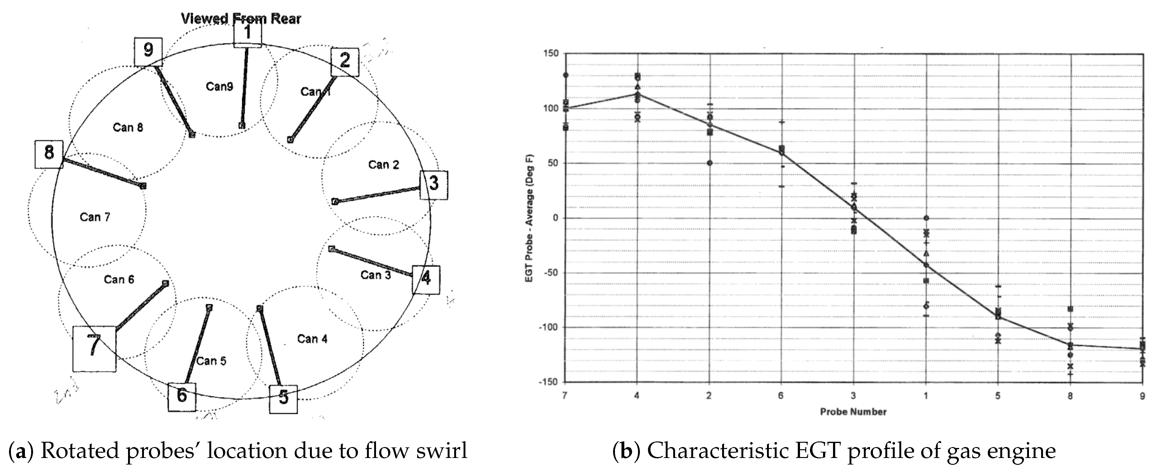
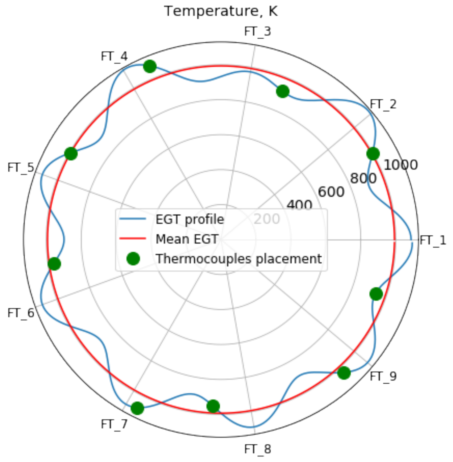
2.3.7. Exhaust Gas Temperature Distribution

We assumed a Gaussian temperature distribution at the end of flame tubes and simulated each flame tube as a heat source with the heat flow and temperature distribution in a circumferential direction, where the x-axis represents the angle from 0 to 360 degrees, as presented in Figure 5. According to our assumption, a breakage in a flame tube leads to a widening of the tube’s temperature profile (in a simplified model), but in fact it is actually more complex. In fact, the mean position of the temperature distribution peak changes too, because burnouts are not symmetrical.

Temperature distributions at the end of each k flame tube were determined as:

$$T(\alpha ,{\alpha }_k)=A\ast exp(\frac{{(\alpha -{\alpha }_k)}^2}{2{\sigma }^2})$$

(24)

and

$${\int }_0^{2\pi }\sum _{k=1}^{9}T(\alpha ,{\alpha }_k)d\alpha =2\pi T_{EGT}$$

(25)

where ${\alpha }_k$ is the angle of the k-th thermocouple placement.

2.4. Tuning of the Gas Turbine Physical Model

Having developed the physics-based model architecture, we tuned its parameters to fit the real operation data of the gas turbine. We used the Nelder-Mead method to minimize the difference between the mass flow rate of the gas turbine from field data and the mass flow rate of the components of the physical model.

As was mentioned above, performance maps determine the operating conditions of turbines and compressors. In the study, the LPC performance map was obtained from the turbine operator, but the maps for other turbine components had to be acquired. We decided to use an optimization algorithm to find the scaling parameters for fitting the performance maps. We used 10 points of the operation data from a different period of the gas turbine’s performance. These points were obtained from the steady-state working conditions of the gas turbine because, in steady state, we can say that the mass flow rates of all compressors and turbines are equal. The optimization algorithm was applied to minimize the following functions:

$$F_j^N\left(R{P}_j\right)=\sum _{i=1}^N{({\dot{m_i}}_{LPC}-{\dot{m_i}}_j\left(R{P}_j\right))}^2$$

(26)

where $R{P}_j$ represents resizing parameters for the $F_j$ function and $j=\overline{1,3}$ corresponds to HPC, HPT, and LPT, respectively. N is the number of points used for optimization, which equals 10.

To determine the exact position of the EGT probes, we used the Nelder–Mead method, optimizing 10 parameters. The algorithm varied the distribution of the temperature at the end of flame tubes determined by the variance and positional angle of the EGT probes to minimize the following goal function:

$$F^N(\sigma ,{\alpha }_1,{\alpha }_2,...{\alpha }_9)=\sum _{j=1}^9{\left[\sum _{i=1}^N\frac{{\widetilde{TC}}_{ij}(\sigma ,{\alpha }_j)-T{C}_{ij}}{N}\right]}^2$$

(27)

where ${\widetilde{TC}}_{ij}(\sigma ,{\alpha }_j)$ and $T{C}_{ij}$ are j simulated and measured temperature on the j-th thermocouple in the i-th experiment.

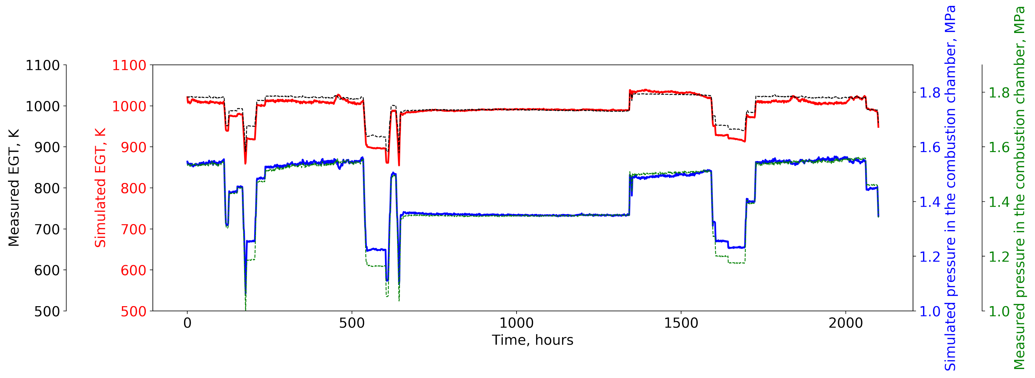
2.5. Model Validation

To validate the tuned model, we simulated the operation of the turbine for 2000 min. Figure 6 compares the field data values and the simulation results of the physical model.

The physics-based model showed good accuracy in the gas turbine’s steady-state regime of work, where the error was less than 2%.

Applying the optimization algorithm to determine the thermocouples’ position allowed us to obtain the optimized function’s value:

$$F^{10}(\sigma ,{\alpha }_1,{\alpha }_2,...{\alpha }_9)=12.15$$

(28)

$$F^{100}(\sigma ,{\alpha }_1,{\alpha }_2,...{\alpha }_9)=10.24$$

(29)

2.6. Hybrid Modeling

After the physics-based model of a gas turbine was created, it was combined with a machine learning model.

Taking into account the lack of labeling (only one label was known when the flame tubes were repaired), we decided to use a machine learning model trained by a physics-based model. In this configuration, we produced much-labeled data, which were then fitted to the machine learning-based model.

The problem and assumptions can be stated as follows:

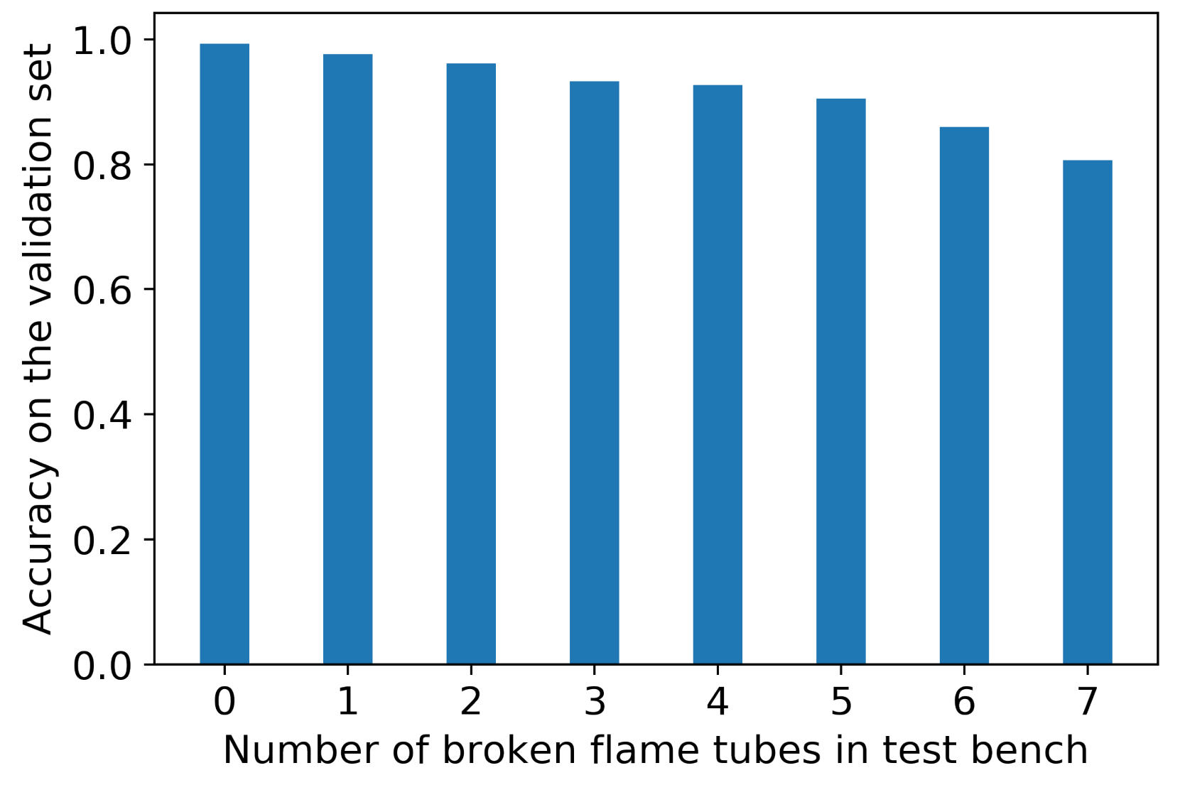
• Nine flame tubes were placed in the combustion chamber. Each could be broken in the same period of time (in the present case study, seven flame tubes were broken simultaneously). The number of broken flame tubes at a given moment may range from zero to nine with unknown probability.
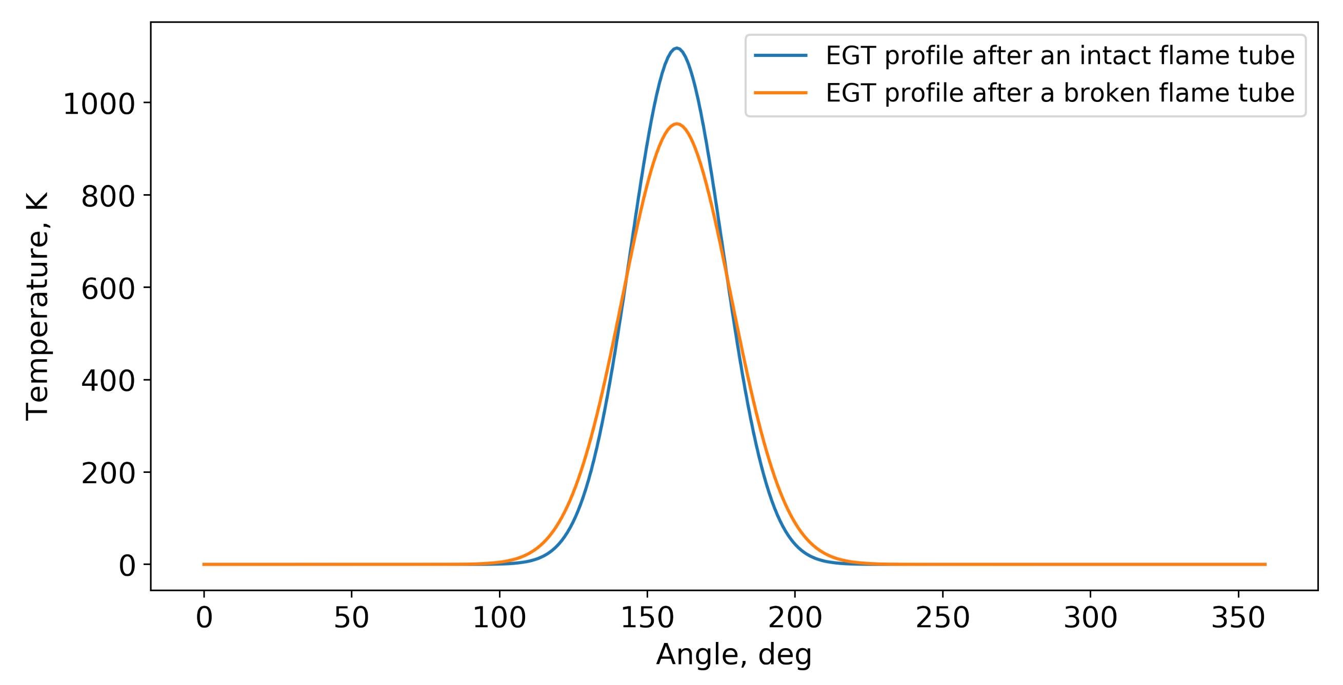
• Malfunction of the flame tubes led to changes in the temperature profile of the EGT probes.
• Malfunction of the different flame tubes led to unique differences in the temperature profile of the EGT probes.

We used neural networks as the architecture for the machine learning model, as they are well suited for multiclass classification problems [30,31]. It was also interesting to check different neural network structures and observe the trainability of the model.

We tried different architectures for the neural networks with different numbers of hidden layers and neurons. Although different architectures produced almost equal results, the neural network with three hidden layers performed the best.

We used two different activation functions in the hidden layers (Rectified Linear Unit (ReLU) and Exponential Linear Unit (ELU)) to compare their performance to possibly improve the results [32,33]:

$$ReLU\left(x\right)=max(0,x)$$

(30)

$$ELU\left(x\right)=\{\begin{array}{cc}x& x>0\\ \alpha (e^x-1)& x<0\end{array}$$

(31)

For the output layer, the sigmoid activation function was used:

$$\sigma \left(x\right)=\frac{1}{1+e^{-x}},prediction=\{\begin{array}{cc}1& \sigma \left(x\right)>0.5\\ 0& \sigma \left(x\right)\le 0.5\end{array}$$

(32)

The inputs to the model were the EGT probes’ temperatures $T_i$ from the physics-based model, and the outputs were nine possible classes $a_j$ corresponding to flame tube malfunctions:

$$input=\left(\begin{array}{c}{T}_1\\ T_2\\ ...\\ T_9\end{array}\right),output=\left(\begin{array}{c}{a}_1\\ a_2\\ ...\\ a_9\end{array}\right),where{a}_j=\{\begin{array}{cc}1& j\mathrm{flame}\mathrm{tube}\mathrm{is}\mathrm{broken}\\ 0& j\mathrm{flame}\mathrm{tube}\mathrm{is}\mathrm{whole}\end{array}$$

(33)

Figure 7 shows the neural network structure.

We used the $Adam$ optimizer [34] and $binarycrossentropy$ loss function [35] for the model. Let [input, hidden layer 1, hidden layer 2, hidden layer 3, output] represent the number of neurons in a network. In this study, we used the following architectures for the model:

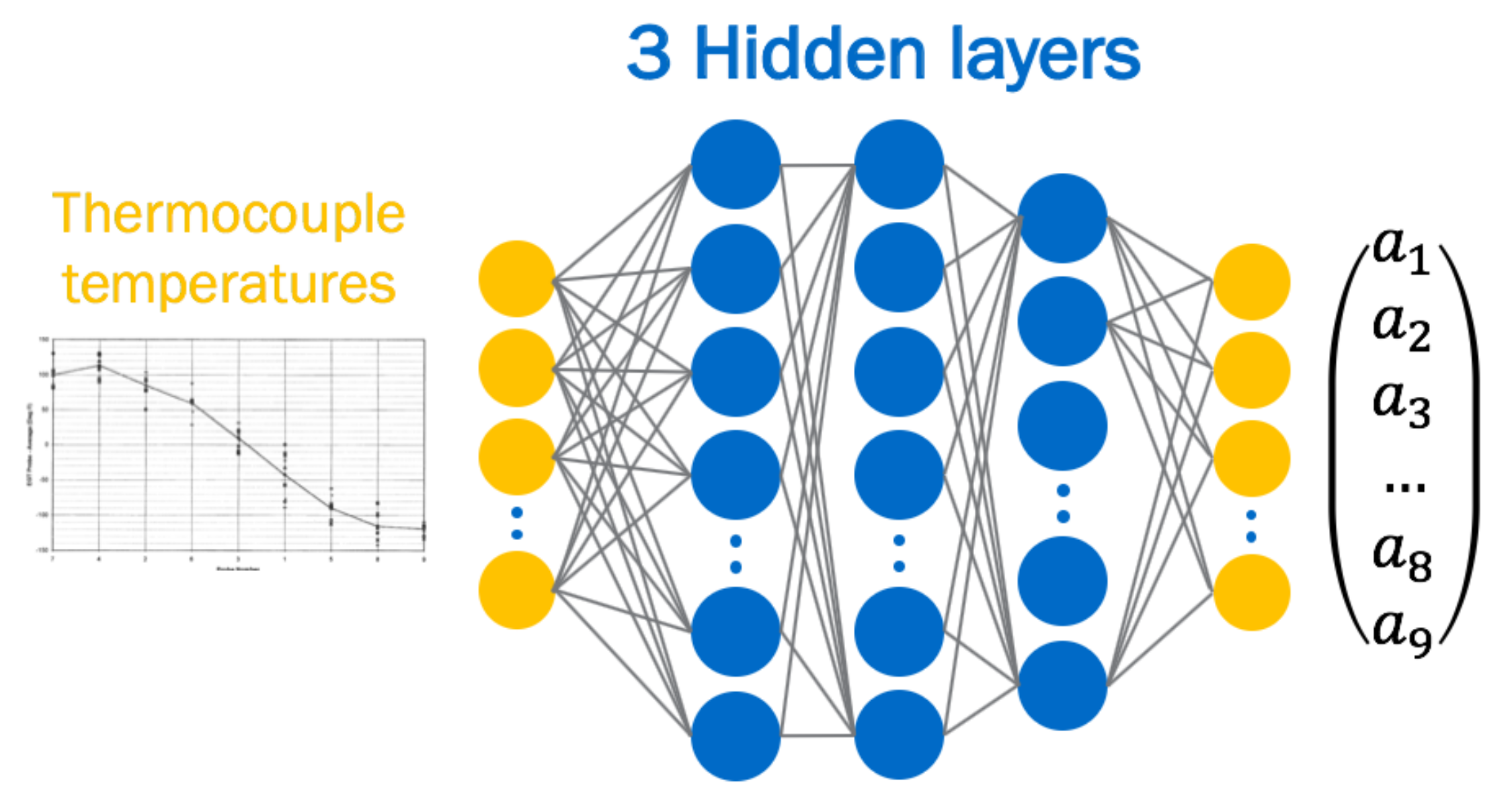
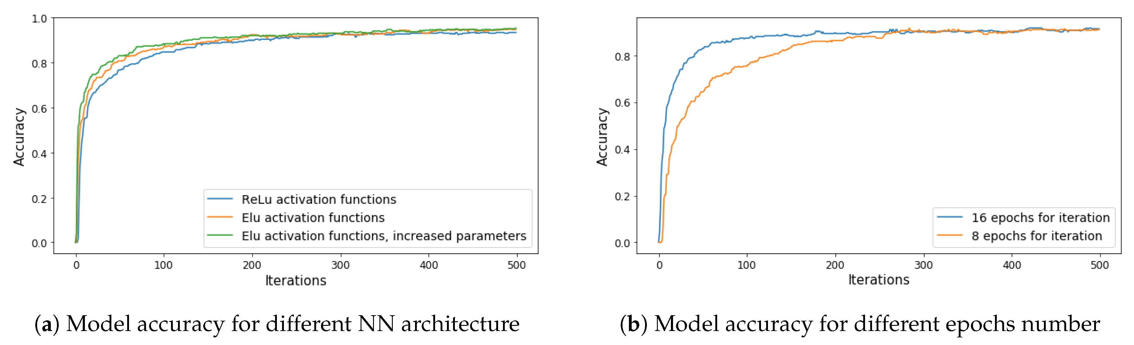
• $[9-50-50-40-9]$, dropout = 0.1, ReLU activation function in hidden layers
• $[9-50-50-40-9]$, dropout = 0.1, ELU activation function in hidden layers
• $[9-70-70-50-9]$, dropout = 0.1, ELU activation function in hidden layers

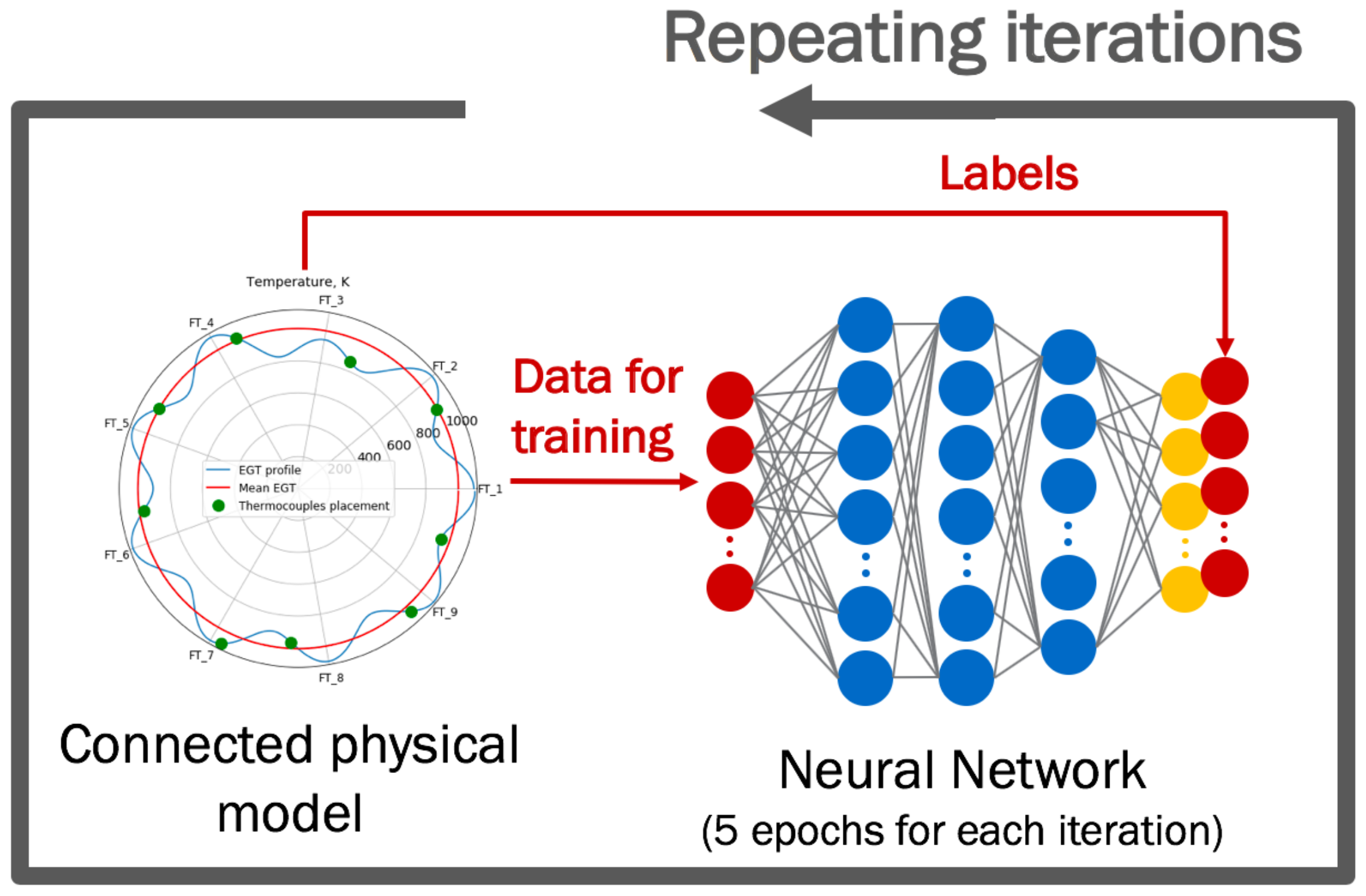
2.6.1. Combination of Approaches for Flame Tubes Health Monitoring

Physics-based and machine learning models were combined in the way in which the physics-based model simulated flame tube breakages. The following algorithm describes the simulation process:

• The physics-based model chose a random number N from zero to nine, which determined the amount of broken flame tubes in the data sample.
• Random flame tubes $n_j,j=\overline{1,N}$ were defined as broken.
• Malfunction in each $n_j$ flame tube was simulated as the increased variance of the temperature distribution. Figure 8 shows an example of the simulated malfunction in the third flame tube.
• The physics-based model simulated the steady-state working conditions of the turbine and calculated the EGT distribution.

In the combined model, the physics-based model generated new labeled data each iteration, which prevented the neural network from overfitting. Figure 9 shows how the physics-based model was connected with the machine learning model.

The model was trained in M iterations. The following Algorithm 1 was used for the training:

Algorithm 1: Training algorithm

We determined the absolute accuracy with the following formula:

$$acc=\frac{{\sum }_{j=1}^M{\sum }_{i=1}^9{p}_{ij}}{9\ast M},where{p}_{ij}=\{\begin{array}{cc}1& {\tilde{a}}_{ij}=a_{ij}\\ 0& {\tilde{a}}_{ij}\ne a_{ij}\end{array}$$

(34)

where $a_{ij}$ is the label for i flame tube in j experiment out of M and ${\tilde{a}}_{ij}$ is the prediction for i flame tube in j experiment out of M.

2.6.2. Model Training and Architectures Comparison

The most important task was to choose the right neural network architecture. We compared the neural networks with different numbers of trainable parameters and hidden layers. Each architecture was trained for 30 iterations, and its accuracy was checked on the same test dataset. The ELU activation function was used in hidden layers. Each architecture was also trained with 15 epochs in each iteration and was fitted with 100 batch sizes.

We investigated the hyperparameters of the neural network with three hidden layers. Each architecture for the model was trained with 500 iterations. The results show good trainability for the model, as presented in Figure 10. The architecture $[9-70-70-50-9]$ with the ELU activation function in hidden layers produced the most accurate results (−0.95).

We have chosen the following hyperparameters for training:

• Epochs number—16.
• Batch size—40.

The mean timing for each iteration shows that the physics-based model, which generates datasets, limits the speed of training:

• Mean time of the dataset generation = 9.6 s for 900 labeled data points.
• Mean time of the neural network training = 1.22 s for 16 epochs.

We considered other metrics as well. In the designed model, we checked the accuracy of the newly generated datasets. However, we considered a more common way to validate the model that generates just one test bench. On this test bench, we applied absolute accuracy and other metrics, such as F1 score, area under the receiver operating characteristic curve (AUC ROC) score, precision score, and recall score [36,37]. Figure 11 shows the results on the accuracy for different metrics. Absolute accuracy showed the same trend with the validation set as with the generated datasets.

The accuracy of the number of broken flame tubes was also investigated. The increase in the number of broken flame tubes complicates the EGT profile, so the model should have a lower accuracy value.

We designed an experiment where the pre-trained model was applied to eight different validation sets consisting of 600 data samples each. In each validation set, the constant number of broken flame tubes was simulated (0, 1, 2, ..., 7 broken flame tubes). Figure 12 shows our hypothesis that the accuracy would decrease with an increased number of simultaneously broken flame tubes was correct.

3. Results and Discussion

The physics-based model was used to train the neural network under various conditions of malfunctioning flame tube, and it achieved an accuracy of more than 0.95. The next step was to validate the model using field data.

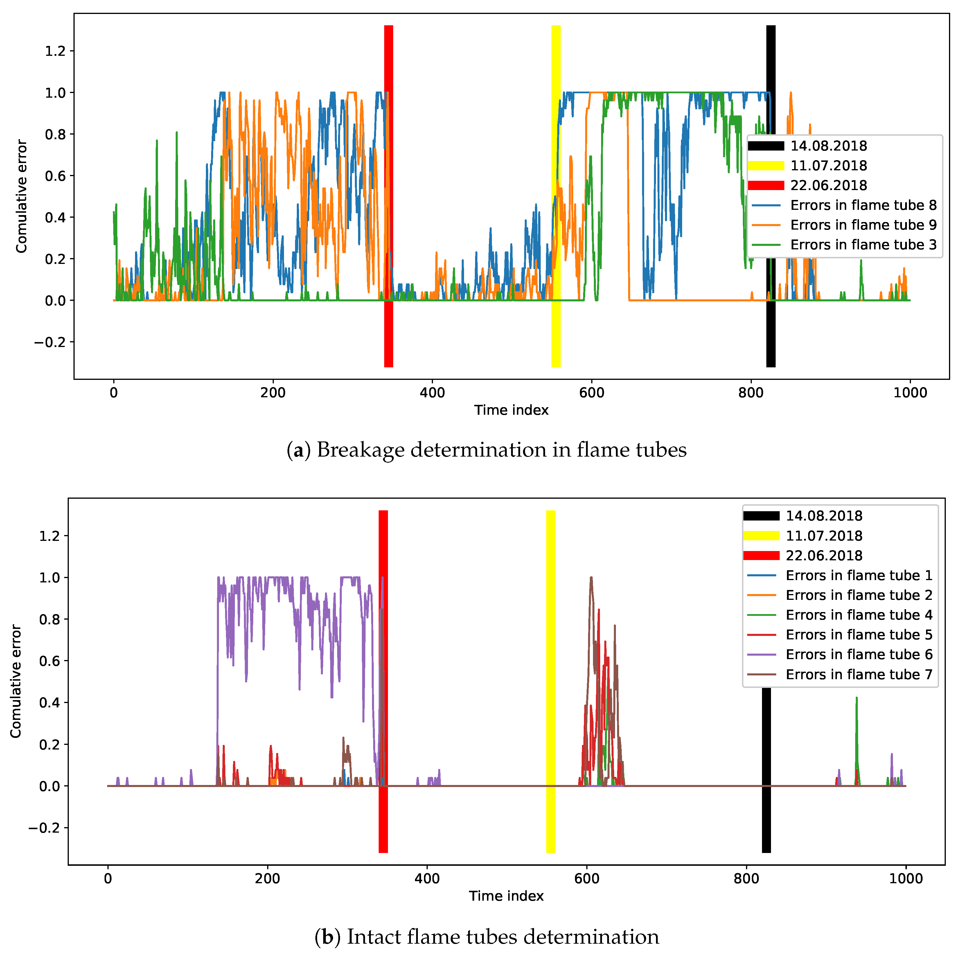
3.1. Prescriptive Results

We applied the model to predict the probability of flame tube malfunction for each field datum point. As the model worked with high accuracy only on steady-state conditions we accumulate the error every 15 min interval. We call it a cumulative error as it presents the whole error during this 15 min working interval (Figure 13). We defined the 15 min interval as time index.

Figure 14 shows the cumulative error over six months for all nine flame tubes. As shown in the figure, we identified three regions for discussion of the predictions. The regions are drawn in Figure 14:

• Black color—14 August 2018. The day when flame tubes 1, 2, 3, 4, 6, 8, 9 were repaired.
• Yellow color—11 July 2018. The day when flame tubes have broken, according to the model prediction.
• Red color—22 June 2018. A previous repair of flame tubes, according to the model prediction.

The application of the model to the FT8 gas turbine dataset correctly determined the breakage time for three broken flame tubes out of seven. False negative results (when the flame tube is broken, but the model predicts it is healthy) may be due to small defects in the replaced flame tubes.

Detecting the deviation in EGT profile from normal behaviour the hybrid model predict the flame tubes’ breakage a month before their repair. This means that the operating company used gas engines with broken flame tubes for about a month.

Between 22 June 2018 and 11 July 2018, some increase in error, Figure 14a, was seen. This increase presumably is linked with the breakage. It is probably connected to injector lag, so the subsequent improvement of the model will allow us to observe the causes in more detail.

The proposed methodology can be applied not only for development of gas turbines but also to any other complex systems, such as pumps, compressors, and turbochargers. The methodology presented in this study may be integrated into maintenance, repair, and overhaul software and may be used during the machinery life cycle for better performance.

3.2. Advantages of Combined Approach

As this work shows, the combined approach makes it possible to predict malfunction for even a very small amount of labeled data. In our case we have only one label for the whole dataset—the date when the flame tubes were replaced. Even so, we use this label not to train the model, but to validate it. The following advantages of the combined approach may be of research interest in this field:

• Only a small amount of the field data is needed to adjust the model to a real turbine. In the case of the FT8 gas turbine, we worked with only 10 data points to identify the performance maps. This means that the model could be tuned to new turbines after a day of operation, which indicates the scalability of the approach.
• Compared with a purely data-driven approach, the combined model allows operators to detect not only the abnormal behavior of gas turbines but also the reasons for it.
• Many malfunctions can be simulated. As soon as the physical model is validated, we can simulate many types of faults.

4. Conclusions

This paper presented the workflow of prescriptive analytics of the gas turbine engine based on its hybrid model. The model utilizes a data-driven and a physics-driven approach. The developed model can accurately identify different malfunctions of the engine based on its performance. However, the presented hybrid approach cannot be implemented without developing a physics-based model that is tuned to fit the performance of a gas turbine. Therefore, the developed model has some limitations:

• Lack of engineering data is the main limitation in the development of a physics-based model. It is not possible to develop a model without performance maps for the compressors and turbines.
• Unknown malfunctions or other malfunctions not taken into during machine learning model training, could be identified incorrectly.
• If the construction of a gas turbine is changed (for instance, if the EGT probes are placed differently), the model has to be adjusted.

References

1. Definition of Prescriptive Analytics—Gartner Information Technology Glossary. Available online: https://www.gartner.com/en/information-technology/glossary/prescriptive-analytics (accessed on 24 October 2020).
2. Lepenioti, K.; Bousdekis, A.; Apostolou, D.; Mentzas, G. Prescriptive analytics: Literature review and research challenges. Int. J. Inf. Manag. 2020, 50, 57–70. [Google Scholar] [CrossRef]
3. Deshpande, P.S.; Sharma, S.C.; Peddoju, S.K. Predictive and Prescriptive Analytics in Big-data Era. In Security and Data Storage Aspect in Cloud Computing; Springer: Berlin/Heidelberg, Germany, 2019; pp. 71–81. [Google Scholar]
4. Matyas, K.; Nemeth, T.; Kovacs, K.; Glawar, R. A procedural approach for realizing prescriptive maintenance planning in manufacturing industries. CIRP Ann. 2017, 66, 461–464. [Google Scholar] [CrossRef]
5. Martins, D.R. Off-Design Performance Prediction of the CFM56-3 Aircraft Engine. Master’s Thesis, Tecnico Lisboa, Lisboa, Portugal, 2015. [Google Scholar]
6. Ghose, P.; Patra, J.; Datta, A.; Mukhopadhyay, A. Prediction of soot and thermal radiation in a model gas turbine combustor burning kerosene fuel spray at different swirl levels. Combust. Theory Model. 2016, 20, 457–485. [Google Scholar] [CrossRef]
7. Durante, A.; Pena-Vergara, G.; Curto-Risso, P.; Medina, A.; Hernández, A.C. Thermodynamic simulation of a multi-step externally fired gas turbine powered by biomass. Energy Convers. Manag. 2017, 140, 182–191. [Google Scholar] [CrossRef] [Green Version]
8. Bilgen, E. Exergetic and engineering analyses of gas turbine based cogeneration systems. Energy 2000, 25, 1215–1229. [Google Scholar] [CrossRef]
9. Allen, C.W.; Holcomb, C.M.; de Oliveira, M. Gas Turbine Machinery Diagnostics: A Brief Review and a Sample Application. In Turbo Expo: Power for Land, Sea, and Air; American Society of Mechanical Engineers: New York, NY, USA, 2017; Volume 50916, p. V006T05A028. [Google Scholar]
10. Wong, P.K.; Yang, Z.; Vong, C.M.; Zhong, J. Real-time fault diagnosis for gas turbine generator systems using extreme learning machine. Neurocomputing 2014, 128, 249–257. [Google Scholar] [CrossRef]
11. Mulewicz, B.; Marzec, M.; Morkisz, P.; Oprocha, P. Failures prediction based on performance monitoring of a gas turbine: A binary classification approach. Schedae Inform. 2017, 26, 21. [Google Scholar]
12. Yan, W.; Yu, L. On Accurate and Reliable Anomaly Detection for Gas Turbine Combustors: A Deep Learning Approach. In Proceedings of the Annual Conference of the Prognostics and Health Management Society, Coronado, CA, USA, 18–24 October 2015; Volume 6, pp. 59–71. [Google Scholar] [CrossRef]
13. Digital Twin: Manufacturing Excellence through Virtual Factory Replication—White Paper by M. Grieves. Available online: https://www.researchgate.net/publication/275211047_Digital_Twin_Manufacturing_Excellence_through_Virtual_Factory_Replication (accessed on 11 August 2020).
14. Madni, A.M.; Madni, C.C.; Lucero, S.D. Leveraging digital twin technology in model-based systems engineering. Systems 2019, 7, 7. [Google Scholar] [CrossRef] [Green Version]
15. Prario, A.; Voss, H. FT8A, a New High Performance 25 MW Mechanical Drive Aero Derivative Gas Turbine. In Turbo Expo: Power for Land, Sea, and Air; American Society of Mechanical Engineers: New York, NY, USA, 1990; Volume 79061, p. V003T07A004. [Google Scholar]
16. Day, W.H. FT8: A High Performance Industrial and Marine Gas Turbine Derived from the JT8D Aircraft Engine. In Turbo Expo: Power for Land, Sea, and Air; American Society of Mechanical Engineers: New York, NY, USA, 1987; Volume 79245, p. V002T03A005. [Google Scholar]
17. Allegorico, C.; Mantini, V. A data-driven approach for on-line gas turbine combustion monitoring using classification models. In Proceedings of the Second European Conference of the Prognostics and Health Management Society, Nantes, France, 8–10 July 2014; pp. 92–100. [Google Scholar]
18. Gas Turbine Power Plants. Available online: https://www.isisvarese.edu.it/wp-content/uploads/2016/03/first-law-of-thermodynamics-for-an-open-system-.pdf (accessed on 11 August 2020).
19. GE primer on GE Gas Turbine Performance Characteristics. Available online: http://ncad.net/Advo/CinerNo/ge6581b.pdf (accessed on 11 August 2020).
20. Dai, X.; Breikin, T.; Gao, Z.; Wang, H. Dynamic modelling and Robust Fault Detection of a gas turbine engine. In Proceedings of the 2008 American Control Conference, Seattle, WA, USA, 11–13 June 2008; pp. 2160–2165. [Google Scholar]
21. Turan, O.; Aydin, H. Exergy-based Sustainability Analysis of a Low-bypass Turbofan Engine: A Case Study for JT8D. Energy Procedia 2016, 95, 499–506. [Google Scholar] [CrossRef] [Green Version]
22. Bălănescu, D.-T.; HriţCu, C.E.; Talif, S.G. Aeroderivative Pratt & Whitney FT8-3 gas turbine—An interesting solution for power generation. Incas Bull. 2011, 3, 9–14. [Google Scholar]
23. Kurzke, J.; Riegler, C. A new compressor map scaling procedure for preliminary conceptional design of gas turbines. In Turbo Expo: Power for Land, Sea, and Air; American Society of Mechanical Engineers: New York, NY, USA, 2000; Volume 78545, p. V001T01A006. [Google Scholar]
24. Cumpsty, N. Jet Propulsion: A Simple Guide to the Aerodynamics and Thermodynamic Design and Performance of Jet Engines; Cambridge University Press: Cambridge, UK, 2003. [Google Scholar] [CrossRef]
25. Energy Efficient Engine High Pressure Compressor—Component Performance Report. Available online: https://ntrs.nasa.gov/citations/19850025825 (accessed on 11 August 2020).
26. Broichhausen, K. Aerodynamic Design of Turbomachinery Components—CFD in Complex Systems; AGARD Lecture Series 195; NATO Science and Technology Organization: Brussels, Belgium, 1994. [Google Scholar]
27. Extended Parametric Representation of Compressor Fans and Turbines. Volume 3: MODFAN User’s Manual (Parametric Modulating Flow Fan). Available online: https://ntrs.nasa.gov/citations/19860014467 (accessed on 11 August 2020).
28. Performance of a High-Work Low Aspect Ratio Turbine Tested with a Realistic Inlet Radial Temperature Profile. Available online: https://ntrs.nasa.gov/citations/19910010813 (accessed on 11 August 2020).
29. NASA Report: Coefficients for Calculating Thermodynamic and Transport Properties of Individual Species. Available online: https://ntrs.nasa.gov/citations/19940013151 (accessed on 16 October 2020).
30. Ding, C.H.; Dubchak, I. Multi-class protein fold recognition using support vector machines and neural networks. Bioinformatics 2001, 17, 349–358. [Google Scholar] [CrossRef] [PubMed] [Green Version]
31. Bhardwaj, A.; Tiwari, A.; Bhardwaj, H.; Bhardwaj, A. A genetically optimized neural network model for multi-class classification. Expert Syst. Appl. 2016, 60, 211–221. [Google Scholar] [CrossRef]
32. Clevert, D.; Unterthiner, T.; Hochreiter, S. Fast and Accurate Deep Network Learning by Exponential Linear Units (ELUs). In Proceedings of the 4th International Conference on Learning Representations, ICLR 2016, San Juan, PR, USA, 2–4 May 2016. [Google Scholar]
33. Pedamonti, D. Comparison of non-linear activation functions for deep neural networks on MNIST classification task. arXiv 2018, arXiv:1804.02763. [Google Scholar]
34. Kingma, D.P.; Ba, J. Adam: A method for stochastic optimization. arXiv 2014, arXiv:1412.6980. [Google Scholar]
35. Understanding Binary Cross-Entropy/Log Loss: A Visual Explanation. Available online: https://towardsdatascience.com/understanding-binary-cross-entropy-log-loss-a-visual-explanation-a3ac6025181a (accessed on 11 August 2020).
36. Shung, K.P. Accuracy, Precision, Recall or F1? 2018. Available online: https://towardsdatascience.com/accuracy-precision-recall-or-f1-331fb37c5cb9 (accessed on 11 August 2020).
37. McClish, D.K. Analyzing a portion of the ROC curve. Med. Decis. Mak. 1989, 9, 190–195. [Google Scholar] [CrossRef] [PubMed]
Figure 1. FT8 gas turbine [16].
Ijtpp 05 00029 g001
Figure 2. Exhaust gas temperature (EGT) probes’ placement and temperature profile characteristics [12].
Ijtpp 05 00029 g002
Figure 3. Workflow for physics-based model of a gas turbine power plant development.
Ijtpp 05 00029 g003
Figure 4. Architecture of the gas turbine model.
Ijtpp 05 00029 g004
Figure 5. Exhaust gas temperature distribution after one flame tube.
Ijtpp 05 00029 g005
Figure 6. Simulated and measured combustion pressure and EGT histories.
Ijtpp 05 00029 g006
Figure 7. Structure of the neural network used for flame tube malfunction detection.
Ijtpp 05 00029 g007
Figure 8. Temperature distribution after LPC turbine with a broken third flame tube.
Ijtpp 05 00029 g008
Figure 9. Architecture of a combined model.
Ijtpp 05 00029 g009
Figure 10. Neural network accuracy.
Ijtpp 05 00029 g010
Figure 11. Accuracy results for different metrics.
Ijtpp 05 00029 g011
Figure 12. Absolute accuracy for different number of broken flame tubes.
Ijtpp 05 00029 g012
Figure 13. Error on field data and cumulative errors for the 4th EGT probe.
Ijtpp 05 00029 g013
Figure 14. Application of the model to predict exact number of broken flame tubes.
Ijtpp 05 00029 g014
Publisher’s Note: MDPI stays neutral with regard to jurisdictional claims in published maps and institutional affiliations.