An Extended Version of an Algebraic Intermittency Model for Prediction of Separation-Induced Transition at Elevated Free-Stream Turbulence Level

Abstract

An algebraic intermittency model for boundary layer flow transition from laminar to turbulent state, is extended using an experimental data base on boundary layer flows with various transition types and results by large eddy simulation of transition in a separated boundary layer. The originating algebraic transition model functions well for bypass transition in an attached boundary layer under a moderately high or elevated free-stream turbulence level, and for transition by Kelvin–Helmholtz instability in a separated boundary layer under a low free-stream turbulence level. It also functions well for transition in a separated layer, caused by a very strong adverse pressure gradient under a moderately high or elevated free-stream turbulence level. It is not accurate for transition in a separated layer under a moderately strong adverse pressure gradient, in the presence of a moderately high or elevated free-stream turbulence level. The extension repairs this deficiency. Therefore, a sensor function for detection of the front part of a separated boundary layer activates two terms that express the effect of free-stream turbulence on the breakdown of a separated layer, without changing the functioning of the model in other flow regions. The sensor and the breakdown terms use only local variables.

1. Introduction

Laminar boundary layer separation, followed by transition to turbulence in the separated layer, is a common phenomenon in low Reynolds number flows over aerofoils and turbomachinery blades. A separated boundary layer becomes unstable and breaks down with the generation of fine-scale turbulence [1]. The resulting small-scale unsteadiness creates increased momentum exchange in the wall-normal direction, and mostly leads to turbulent boundary layer reattachment with formation of a separation bubble. In a free stream with a low turbulence level, the inherent instability of the separated layer leads to transition after separation. The transition is accelerated in the presence of elevated free-stream turbulence, due to perturbations by fluctuations from the free stream [2,3].

A small increase in flow incidence may cause an abrupt increase in the bubble length and a significant loss increase in an aerodynamic flow with low turbulence level. This process is typically referred as bubble bursting [4]. Thus, proper accounting for boundary layer separation and transition is important for aircraft design and operation. In low pressure turbines of aero-engines, the chord-based Reynolds numbers are relatively low. So large portions of the boundary layers are laminar. The main consequences of this are for suction surface boundary layers, which are subjected to an adverse pressure gradient. The laminar boundary layer may separate and cause a significant decrease in efficiency. Thus, proper accounting for transition in attached and separated boundary layers is also important for turbomachinery flows.

2. Phenomena in Transitional Separated Boundary Layers

The flow phenomena during transition from laminar state to turbulent state in a separated boundary layer, subjected to an adverse pressure gradient, under various levels of free-stream turbulence, were recently reviewed by Z. Yang [5], based on direct numerical simulation (DNS) by McAuliffe and Yaras [6] and Balzer and Fasel [7] and experimental results by Simoni et al. [8] and Istvan and Yarusevych [9]. The findings were subsequently summarized by Li and Yang [10] and further interpretation was added, gained from large eddy simulation results (LES) by these authors. Based on the discussion by Li and Yang and conclusions from DNS by Hosseinverdi and Fasel [11], we summarize the relevant phenomena hereafter.

In this paper, turbulence levels are categorised as low, moderately high and elevated for free-stream turbulence intensities at the position of transition lower than about 1%, in the order of 2% to 3%, and higher than about 4%. Adverse pressure gradients are quantified by the pressure gradient parameter K = −10⁶νU⁻²(dU/dx) at the position of transition, where ν is the kinematic viscosity, U is the magnitude of the velocity at the boundary layer edge and dU/dx is the corresponding stream-wise gradient. The pressure gradient levels are quantified by the terms mild, moderately strong and strong for K-values of about one, two and three.

Under a very low or low free-stream turbulence level, rolls are formed by Kelvin–Helmholtz instability in a separated laminar boundary layer (primary instability). At their origin, they cover the full span of the separated layer, group into pairs while they travel downstream, and become unstable themselves by spanwise perturbations (secondary instability). The secondary instability causes breakdown, leading to the production of turbulence. Unless the adverse pressure gradient is very strong, the separated layer, after becoming turbulent, reattaches due to increased momentum transfer in the transversal direction.

Under increased free-stream turbulence, streaky structures, called Klebanoff streaks, develop in the attached part of the boundary layer upstream of separation. These are zones alternating in a spanwise direction with a streamwise velocity larger than the mean value (positive streak) and with a streamwise velocity lower than the mean value (negative streak) [12]. The streaks are induced by penetration into the laminar boundary layer of low-frequency components of fluctuations from the free stream, while high-frequency components are filtered out. The low-pass filtering by the laminar layer is called the shear-sheltering effect [13,14]. The streaks are elongated in the streamwise direction and have a spanwise width comparable to the boundary layer thickness. Under a weak or mild adverse pressure gradient, without boundary layer separation, the streaks cause transition in attached boundary layer state. This form of transition is categorised as bypass transition, meaning that the instability patterns of Tollmien–Schlichting type, which occur under low free-stream turbulence in an attached boundary layer, are bypassed. When the boundary layer separates, the Klebanoff streaks perturb the Kelvin–Helmholtz rolls. When the streaks reach sufficient strength due to excitation by the free-stream turbulence, they break the rolls up into part-span rolls. The breakdown of the separated layer is then much faster.

In the past, this last type of transition in separated state was often described as being of bypass type with the meaning that it was believed that the Klebanoff steaks suppress the Kelvin–Helmholtz rolls. However, the research by McAuliffe and Yaras [6], Balzer and Fasel [7], Simoni et al. [8] and Istvan and Yarusevych [9] has proven that this does not happen. The Kelvin–Helmholtz rolls stay present in the separated boundary layer, but the Klebanoff streaks distort the rolls and break them into parts with formation of part-span rolls. The higher the free-stream turbulence level is, the more intense the distortions by the Klebanoff streaks are, the faster the Kelvin–Helmholtz rolls split into parts and the faster the final breakdown leading to turbulence is. So, streaks and rolls interact in the transition process. The transition may still be categorised as being of bypass type, but with the meaning that the spontaneous secondary instability phase by spanwise patterns of full-span Kelvin–Helmholtz rolls, which occurs under a low free-stream turbulence level, is bypassed, but not the primary instability of the separated boundary layer leading to the creation of the rolls themselves.

Increased free-stream turbulence and an increased adverse pressure gradient cause stronger growth of the Klebanoff streaks, both in the attached part of the boundary layer upstream of the separation and in the front part of the separated boundary layer, downstream of the separation. McAuliffe and Yaras [6] showed that an instability by local inflectional velocity profiles develops in a separated boundary layer perturbed by streaks. It is similar to the Kelvin–Helmholtz instability under a low turbulence level, but it results in part-span rolls. The instability leads to the formation of a series of vortex loops—similar to a turbulent spot in an attached boundary layer—and causes entrainment of fluid towards the wall. As a result, a patch of turbulent boundary layer develops downstream. Coull and Hodson [15] also observed the development of part-span rollup eddies in a separated boundary layer perturbed by moving wakes. They concluded that both streaks and part-span Kelvin–Helmholtz rolls contribute to earlier transition under wake impact.

Further insight in the role of the streaks and the part-span rolls has been obtained by the DNS of Hosseinverdi and Fasel [11]. They showed that both have a role, but that the effect of the rolls is the largest at the lower free-stream turbulence level, while the effect of the streaks is the largest at larger free-stream turbulence level. Under lower free-stream turbulence, transition is dominated by Kelvin–Helmholtz rolls, which are broken into part-span rolls by the Klebanoff streaks, leading to faster breakdown than with full-span rolls. Under higher free-stream turbulence, the process of breaking the rolls into parts is stronger, but the streaks also cause the boundary layer breakdown directly.

3. Quantification of the Effects Causing Transition in Separated Boundary Layers

The conclusion from the above description of the phenomena is that a transition model connected to the Reynolds-averaged Navier–Stokes equations (RANS), meant for transition in a separated boundary layer subjected to an adverse pressure gradient and to moderately high or elevated free-stream turbulence, has to express the growth of perturbations by the combined effects of Kelvin–Helmholtz rolls and Klebanoff streaks and has to express when the distortion of the separated boundary layer becomes sufficiently strong for causing transition. Therefore, the effects of free-stream turbulence level, adverse pressure gradient magnitude and flow Reynolds number have to be quantified. Clearly, the higher the turbulence level, the faster the transition occurs.

The effect of the adverse pressure gradient is less clear from the research cited up to now, because the pressure gradient was not varied in any of the research studies. More insight comes from the recently composed experimental data base by Simoni et al. [16], on boundary layer flows on a flat plate, with four turbulence levels, four adverse pressure gradient levels and three Reynolds numbers and the interpretation of the effects by Dellacasagrande et al. [2,3].

Starting from a case with a rather strong adverse pressure gradient, it is observed that by lowering the adverse pressure gradient, the separation point is delayed, and the separated zone becomes longer. The explanation for this last phenomenon is that under the same level of free-stream turbulence and the same Reynolds number, the boundary layer is somewhat thicker at separation by the delayed separation, which makes the size of the Kelvin–Helmholtz rolls somewhat larger and their evolution path, thus, somewhat longer. This means that the size of the separation bubble scales with the thickness of the boundary layer at separation under a varying adverse pressure gradient. This scaling effect is clear from the correlations constructed by Dellacasagrande et al. [2,3] for the distance between the position of separation and the start of breakdown and for the distance between the start of breakdown and the position of reattachment. These correlations, in the form of a distance Reynolds number as a function of the momentum thickness Reynolds number and the free-stream turbulence level at the point of separation, do not contain the magnitude of the adverse pressure gradient.

The effect of the Reynolds number is somewhat similar. With a larger Reynolds number, the position of separation only changes slightly under an unchanged adverse pressure gradient and free-stream turbulence level, and the height and length of the separation bubble become smaller. This means that under a varying Reynolds number, the size of the bubble also scales with the thickness of the boundary layer at separation, which becomes lower with an increased Reynolds number.

From the correlations determined by Dellacasagrande et al. [2,3], the scaling effects can be seen. For the distances between separation and start of transition (ST) and transition to reattachment (TR), the correlations are Re_ST = 44.5${Re}_{\theta s}^{0.65}$/Tu^0.5 and Re_TR = 146${Re}_{\theta s}^{0.9}$, and these correlations express similar tendencies as earlier constructed ones. The adverse pressure gradient and flow Reynolds number are not explicit in the correlations, but the effect of these parameters is present by the use of distance Reynolds numbers and the dependence on the momentum thickness Reynolds number at separation, Re_θs. The scaling with the momentum thickness at separation is clear, but the proportionality is less than linear. The effect of the free-stream turbulence level on the length of the instability zone (ST) of the separated layer is explicit.

The primary effect of an increased free-stream turbulence level is that the Klebanoff streaks become stronger upstream and downstream of the separation. The separation position remains almost the same under an unchanged adverse pressure gradient and Reynolds number, but the breakdown of the separated layer is faster with stronger streaks. The unchanged position of separation is a confirmation of the feature, seen earlier with the bypass transition in an attached boundary layer state, that streaks are perturbations without noticeable associated Reynolds stress. From the correlations, it can be deduced that the free-stream turbulence level does not influence the distance between the start of breakdown and reattachment. It means that the free-stream turbulence affects the front zone of the separated boundary layer, which is the instability zone, but not the rear zone which is the zone of recovery towards attached state. This difference in behaviour is also visible in the DNS results by McAuliffe and Yaras [6] and Hosseinverdi and Fasel [11].

4. Transition Models Combined with Turbulence Models

There are three main categories of transition models combined with turbulence models in RANS flow description. In their basic form, they are designed for modelling bypass transition in an attached boundary layer state under a moderately high and elevated free-stream turbulence level and for modelling transition in a separated state by Kelvin–Helmholtz instability under low free-stream turbulence level. Hereafter, we summarize the main characteristics of the categories. For details we refer to the review paper by Dick and Kubacki [17].

Two categories use the concept of intermittency, γ, which is a variable equal to zero in laminar flow and equal to unity in turbulent flow. It is mostly used as a multiplier of the production term(s) of a turbulence model. These terms are suppressed in laminar flow, grow in a transitional boundary layer and recover their full strength in turbulent flow. In most models, the intermittency is obtained from a transport equation (Menter et al. [18], Langtry et al. [19], Ge et al. [20], Menter et al. [21]). However, an intermittency factor may also be expressed by an algebraic formula, either as a function of streamwise distance (Fürst et al. [22]) or as a function of wall-normal distance (Kubacki and Dick [23,24]).

Most models using the intermittency concept employ empirical correlations in the equation for intermittency, but some obtain the intermittency by sensor quantities that are representative for some types of transition (Ge et al. [20], Kubacki and Dick [23,24]). With intermittency-based models, separation-induced transition is frequently described by a supplementary production term. An example is the model by Menter et al. [21] with an additional production term in the k-equation expressing the breakdown due to Kelvin–Helmholtz instability.

A third category of transition models employs a transport equation for laminar fluctuation kinetic energy in a laminar boundary layer perturbed by free-stream turbulence (Walters and Cokljat [25], Pacciani et al. [26], Lopez and Walters [27]). The breakdown process is modelled by equal and opposite transfer terms in the laminar and turbulent fluctuation kinetic energy transport equations. Some models have specific terms for transition in separated state (Pacciani et al. [26]), but some do not have such terms, yet capture the transition to some extent (Walters and Cokljat [25]).

In the present work, an extended version of the algebraic intermittency model by Kubacki and Dick [24] is presented, aimed at improving the predictive qualities for separation-induced transition under moderately high and elevated free-stream turbulence levels. The extension was made thanks to an experimental data base on boundary layer flows on a flat plate under various Reynolds numbers, turbulence intensity levels and pressure gradients by Simoni et al. [16], and thanks to a large eddy simulation (LES) of transition in a separated boundary layer on a flat plate under a moderately high free-stream turbulence level and a very strong adverse pressure gradient by Li and Yang [10].

5. Formulation of the Algebraic Intermittency Model

The transport equations for the turbulent kinetic energy, k, and specific dissipation rate, $\omega$, have the same form as in the previous model version [24]. The basic equations are those of the $k-\omega$ turbulence model by Wilcox [28,29], but the production term in the k-equation is adapted for simulation of transition. The previous model version was designed for simulation of bypass transition in attached boundary layer state and for simulation of transition in separated boundary layer state under low free-stream turbulence. Two changes are made for the extension to transition in a separated boundary layer under moderately high and elevated free-stream turbulence.

The transport equations are:

$$\frac{Dk}{Dt}={\gamma }_{eff}{P}_k+P_{sep}-{\beta }^{*}k\omega +\frac{\partial }{\partial x_j}\left[\left(\nu +{\sigma }^{*}\frac{k}{\omega }\right)\frac{\partial k}{\partial x_j}\right],$$

(1)

$$\frac{D\omega }{Dt}=\alpha \frac{\omega }{k}{P}_k-\beta {\omega }^2+\frac{\partial }{\partial x_j}\left[\left(\nu +\sigma \frac{k}{\omega }\right)\frac{\partial \omega }{\partial x_j}\right]+\frac{{\sigma }_d}{\omega }\frac{\partial k}{\partial x_j}\frac{\partial \omega }{\partial x_j}.$$

(2)

The coefficient β = f_ββ₀, where the function f_β is equal to unity in two-dimensional flows and takes a value lower than unity in round jets. The coefficients α, β₀, β*, σ, σ* and σ_d are constants [28,29]. The first production term in the k-equation is γ_effP_k = γ_effν_sS², where γ_eff is an effective intermittency factor, ν_s is the eddy-viscosity of the small-scale turbulence (defined below by Equation (13)) and $S=\sqrt{2S_{ij}{S}_{ij}}$ is the magnitude of the shear rate tensor S_ij. We also use the magnitude of the rotation rate tensor $\mathsf{\Omega }=\sqrt{2{\mathsf{\Omega }}_{ij}{\mathsf{\Omega }}_{ij}}$. The first production term is the main term for modelling all kinds of transition. It is started by the intermittency factor, γ_eff. The second production term, P_sep, is a boosting term, which has a role in modelling of transition in a separated boundary layer. The expressions of the intermittency factor, γ_eff, and the boosting term, P_sep, are extended with respect to these in the previous model version (defined below by Equations (7) and (8)).

Bypass transition in an attached boundary layer is modelled by two ingredients. The first is splitting of the turbulent kinetic energy k into a small-scale part k_s and a large-scale part k_i by

$$k_s=f_{SS}k,k_l=k-k_s.$$

(3)

The filtering is realised with the shear-sheltering function [24]:

$$f_{SS}=exp\left[-{\left(\frac{C_{SS}\nu }{\sqrt{k}y}\right)}^2\right],\mathrm{with}{C}_{SS}=C_S\left(1+f_k\chi \right),$$

(4)

where χ and f_k account for curvature effects:

$$\chi =tanh\left(\frac{-\mathsf{\Omega }\left(S-\mathsf{\Omega }\right)}{C_{\chi }{\left({\beta }^{\ast }\omega \right)}^2}\right), f_k=1-tanh\left(\frac{k}{C_k\nu \omega }\right).$$

(5)

The values of the constants C_S, C_χ and C_k (see

Table 1. Transition model constants.

Bypass Transition
Aγ	CS		Cχ		Ck		a2
12.0	21.0		10.0		6.0		0.60
Separation-Induced Transition
CKH	AKH	CKlebP	CKlebγ	aω	bω	aγ	bγ	aKleb
2	550	0.01	0.3	150	5	0.95	150	1

) are the same as in the previous model version [24]. The shear-sheltering term (4) expresses the damping of small-scale turbulent fluctuations by the shear in a laminar boundary layer, according to the observations by Jacobs and Durbin [13,14]. With the shear-sheltering function (Equation (4)), the large-scale turbulent fluctuations, with fluctuation kinetic energy k_l (Equation (3)), are allowed to penetrate into the near-wall zone of a laminar boundary layer. These large-scale fluctuations generate the streaks, which are laminar fluctuations. The small-scale turbulent fluctuations are confined to the upper zone of a laminar boundary layer and contribute to the production of turbulence by the production term γ_effP_k = γ_effν_sS².

The shear-sheltering function in the form (4) was introduced by Walters and Cokljat [25] for splitting turbulent fluctuations in small-scale and large-scale parts. However, in their modelling approach, there is an additional equation for laminar fluctuation kinetic energy. In the model used here, laminar fluctuations are not described.

When the turbulent kinetic energy, k, reaches a critical value in the upper zone of a laminar boundary layer, production of turbulence is started deeper in the boundary layer by activation of the intermittency factor by

$$\gamma =min\left(max\left(\frac{\sqrt{k}y}{A_{\gamma }\nu }-1,0\right),1\right).$$

(6)

This activation models the transition.

The value of the constant A_γ (see Table 1) is the same as in the previous model version. In the previous version of the model γ_eff = γ, which is now extended into

$${\gamma }_{eff}=max\left[\gamma ,C_{Kleb\gamma }{f}_{sep}\right],$$

(7)

where f_sep is a new function with a role in modelling of transition in a separated boundary layer and C_Klebγ is a new model constant. The function f_sep is bounded by unity and the constant C_Klebγ is lower than unity. We detail f_sep later (see the later Equation (10)). It is zero in an attached laminar boundary layer, such that the modelling of bypass transition in an attached laminar boundary layer is not changed. The activation of the intermittency is the second ingredient in the modelling of bypass transition. It expresses the excitation of the streaks by the fine-scale turbulence in the edge zone of a laminar boundary layer, leading to the breakdown. After transition completion, the intermittency becomes unity in the turbulent part of a turbulent boundary layer. It stays zero at the wall and evolves towards unity inside the viscous sublayer. So, k_s represents the full turbulent kinetic energy in the turbulent part of a turbulent boundary layer. We refer to Kubacki and Dick [23] for an illustration of the functioning of the bypass model in an attached boundary layer.

The second production term in the k-equation is P_sep. It is a boosting term with a role in modelling of laminar-to-turbulent transition in a separated boundary layer. With respect to the previous model version, it is extended into

$$P_{sep}=max\left[\left(1-\gamma \right)C_{KH}{f}_{KH},C_{KlebP}{f}_{sep}\right]\nu S^2.$$

(8)

The first term between brackets, (1 − γ)C_KHf_KH, is the term for separation-induced transition in the previous model version. It expresses breakdown due to Kelvin–Helmholtz instability under a low free-stream turbulence level. It is a similar term as in the intermittency model by Menter et al. [21] and has been borrowed from that model:

$$f_{KH}=min\left(max\left(\frac{R_V}{2.2A_{KH}}-1,0\right),1\right),\mathrm{with}{R}_V=\frac{y^{2}S}{\nu }.$$

(9)

The term becomes active when the “vorticity Reynolds number”, R_V, reaches a critical value set by the constant A_KH, which may occur inside a separated layer due to the combination of the magnitude of the shear rate and the distance to the wall. This term has been maintained in the current model version. The f_KH-function is active in a separated boundary layer under a sufficiently strong adverse pressure gradient, but it only contributes to the P_sep-term when the local turbulence level is very low and thus, the activity zone of the f_sep-term stays small. This typically happens for separation near a trailing edge under a low free-stream turbulence level, which can be understood from the behaviour of the f_sep-function, discussed hereafter. The values of the constants A_KH and C_KH (see Table 1) are the same as in the previous model version. The function f_sep is the same as in the expression of the effective intermittency (Equation (7)) and C_KlebP is a new model constant.

The model functions without the extension by the f_sep-terms for bypass transition in attached boundary layer state, for transition in a separated layer caused by a moderately strong or strong adverse pressure gradient under a low free-stream turbulence level and for transition in a separated layer caused by a very strong adverse pressure gradient under a moderately high or elevated free-stream turbulence level. The first and second ways of functioning are as explained above, by the γ-expression (6) and the f_KH-term (9). The third functioning comes also from the γ-expression. The intermittency is also activated when a large value of k appears together with a relatively large value of the distance to the wall, which occurs with a large separation zone caused by a very strong adverse pressure gradient combined with a high free-stream turbulence level.

The previous model version has no ingredient for transition in a separated state, under a moderately strong adverse pressure gradient, in the presence of a moderately high or elevated free-stream turbulence level. The previous model version functions for such combinations of flow parameters, but the predictions are not very accurate, as will be shown later. For improving the modelling of transition in a separated boundary layer, with this combination of adverse pressure gradient and free-stream turbulence level, we define the function f_sep, which detects a separated boundary layer. It is the product of two functions:

$$f_{sep}=f_{\gamma }{f}_{\omega },$$

(10)

with

$$f_{\gamma }=\frac{1}{1+exp\left[b_{\gamma }\left(\gamma -a_{\gamma }\right)\right]},f_{\omega }=\frac{1}{1+exp\left[-b_{\omega }\left({Re}_{\omega }-a_{\omega }\right)\right]}.$$

(11)

By the value a_γ = 0.95, the f_γ-function is zero in the outer zone of a laminar boundary layer, also a separated one, in the turbulent part of an attached turbulent boundary layer and in the free stream. The b_γ = 150 value determines the (strong) steepness of this function. The f_γ-function is near to unity close to a wall.

At walls, the boundary conditions of k and ω are [28,29]:

$$k=0\mathrm{and}\omega =6\nu /\left({\beta }_0{y}^2\right).$$

(12)

The set of k–ω Equations (1) and (2) has a solution with eddy-viscosity equal to zero, thus a laminar-flow solution. It is of form k ~ y^3.31 in wall vicinity together with the expression of ω in Equation (12). This solution is thus valid near a wall. Therefore, k = 0 is imposed at the wall itself and ω according to Equation (12) is imposed in the first cell centre next to a wall.

The Reynolds number Re_ω = ωy²/ν is about 85 in the wall’s vicinity due to the wall boundary condition of ω. This Reynolds number stays near to 85 in a large part near the wall of an attached laminar boundary layer and in the viscous sublayer of a turbulent boundary layer and it evolves to a larger value at the edge of an attached laminar boundary layer and in the turbulent part of a turbulent boundary layer. By the value a_ω = 150, the f_ω-function is near to unity away from a wall, outside an attached laminar boundary layer and outside the viscous sublayer of an attached turbulent boundary layer. The value b_ω = 5 determines the steepness of this function. The f_ω-function is near to zero close to a wall. By the value a_ω = 150, the f_ω-function reaches unity away from a wall, but still inside a separated laminar boundary layer, if this layer is sufficiently far away from the wall and if the free-stream turbulence level is sufficiently high. This way, the product of the f_γ- and f_ω-functions becomes different from zero in the outer zone of a separated laminar boundary layer under moderately high or elevated free-stream turbulence. The value of a_ω = 150 is quite critical for obtaining this property. We discuss the choice of a_ω in the next section on the tuning of the model.

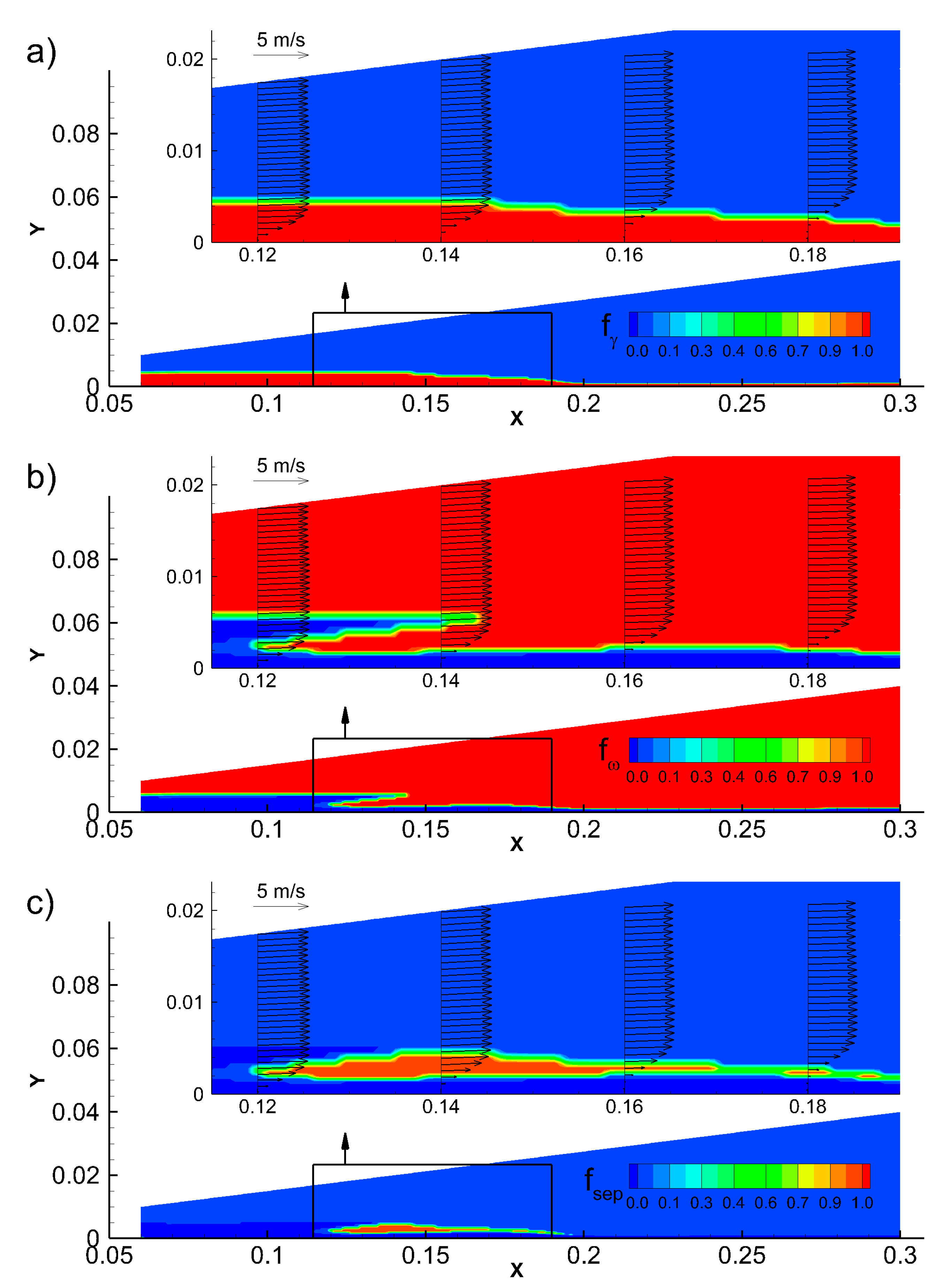
Figure 1 shows contour plots of the f_γ- and f_ω-functions and the resulting f_sep-function in the flow on a flat plate under a moderately strong adverse pressure gradient and a moderately high free-stream turbulence level (a case with boundary layer separation from the data base by Simoni et al. [16] with Tu ≈ 2.5% at the separation point), simulated using the extended model. The magnified views show superimposed velocity vectors (on selected lines) on the contour levels. The separation bubble starts around x = 0.12 m and ends around x = 0.21 m. The f_γ-function is active inside the boundary layer in the laminar state and inside the viscous sublayer in the turbulent state. The f_ω-function is active in the outer zone of the boundary layer and the free stream. The resulting f_sep-function is active in the outer zone of the separated laminar boundary layer and mainly in the front part of the separation bubble. The figure illustrates that by activation of production of turbulent kinetic energy in the zone defined by the f_sep-function, transition may be numerically simulated. Transition starts at the end of the zone defined by the f_sep-function (close to x = 0.18 m). The precise mechanism will be illustrated in the next section (see Figure 2).

The f_sep-function is used in two ways for modelling transition in a separated boundary layer, implemented by the two technically possible ways for changing the source term in the equation of turbulent kinetic energy with the previous version of the model. The first way is by combining f_sep with the expression of the intermittency for bypass transition in the effective intermittency, γ_eff (Equation (7)). Transition is then imposed quite directly, but even with a quite large value of C_Klebγ (we obtain C_Klebγ = 0.3 by tuning), the effect of the intermittency is not immediate, because γ_eff multiplies ν_sS² and the small-scale eddy viscosity, ν_s, is very small at the start of separation due to the damping by the shear-sheltering function f_SS. So, the development of the turbulent kinetic energy, k, needs some flow distance and the rate of development depends on the free-stream turbulence level. The second way of using f_sep is in the boosting term P_sep (Equation (8)). C_KlebP is set at a low value (we obtain C_KlebP = 0.01 by tuning). The boosting term is small, but it is active in the whole area where f_sep is active, because the coefficient in P_sep multiplies νS², with ν the molecular viscosity coefficient. There is thus a small production of turbulent kinetic energy, which finally triggers the intermittency function, γ (Equation (6)). The flow distance needed for reaching the triggering depends on the free-stream turbulence level.

The two ways of using f_sep have a different purpose. The P_sep-term acts quite gradually. By the f_sep-term with coefficient C_Klebγ (Equation (8)), we intend to express the gradually accelerated breakdown by the earlier splitting of the full-span Kelvin–Helmholtz rolls into part-span rolls by the Klebanoff streaks, when these increase in strength. The intermittency function acts more directly. With the f_sep-term with coefficient C_Klebγ in the intermittency expression (Equation (7)), we intend to express the accelerated breakdown of the separated layer by the direct effect of the Klebanoff streaks. Both actions by the Klebanoff streaks become stronger under the combined effects of a large adverse pressure gradient and a large free-stream turbulence level.

Both ways of using f_sep express explicitly the influence of the free-stream turbulence level, but there is no explicit influence of the Reynolds number and the adverse pressure gradient in the modelling terms by f_sep. However, the Reynolds number and the pressure gradient are taken into account in the production of turbulent kinetic energy, because these parameters determine the thickness of the boundary layer at the separation position and thus the size of the activity zone of the f_sep-function. The scaling effects of the Reynolds number and the adverse pressure gradient are thus taken into account.

The way of modelling transition in a separated boundary layer does not correctly express the process of development of perturbations by Kelvin–Helmholtz rolls and Klebanoff streaks, because these are actually coherent fluctuations which do not create turbulent shear stress. They are thus, laminar fluctuations, which in a laminar fluctuation kinetic energy model contribute to the laminar fluctuation kinetic energy. In the current model, there is some Reynolds stress produced in the instability zone of a separated laminar boundary layer, which is physically not present. This should be taken into account in the interpretation of the results of skin friction or boundary layer shape factor.

The small- and large-scale turbulent viscosities are obtained by:

$${\nu }_s=\frac{k_s}{{\tilde{\omega }}_s}, \mathrm{with} {\tilde{\omega }}_s=max\left[\omega ,C_{lim}\frac{S}{f_{sep}{a}_{Kleb}+(1-f_{sep})a_1}\right],$$

(13)

$${\nu }_l=\frac{k_l}{{\tilde{\omega }}_l}, \mathrm{with} {\tilde{\omega }}_l=max\left[\omega ,C_{lim}\frac{S}{a_2}\right].$$

(14)

The eddy viscosity in the Navier–Stokes equations is ν_T = ν_s + ν_l The expressions contain a stress limiter, which limits the eddy viscosity in zones where ω becomes rather small, which mainly happens in reattachment zones of separated layers. The values in the k–ω turbulence model by Wilcox [28,29] are C_lim = 7/8 and a₁ = 0.3. The value of a₁ was determined by Wilcox by tuning the reattachment length of a turbulent boundary layer separating from a backward-facing step. Without the limiter, the eddy viscosity is too large, and the separation zone is too short.

The limiter value in the large-scale eddy viscosity expression (14) is higher: a₂ = 0.6. This value has only a small influence on the reattachment length of a separated layer, because the large-scale part of the turbulence is then very small, but it critically determines the speed by which a boundary layer evolves towards a fully turbulent boundary layer after activation of bypass transition. With a₂ = 0.3, the recovery to a fully turbulent layer is too slow. Moreover, the skin friction stays below the value produced by the original k–ω model. This last effect is caused by the intermittency factor (Equation (6)) which sets γ to zero in the viscous sublayer and thus reduces the production of turbulent kinetic energy in wall proximity with respect to the production by the original turbulence model. In order to compensate the deficit, the shear stress limiter, a₂, of the large-scale turbulence (Equation (14)) has to be enlarged with respect to the limiter, a₁, of the unmodified model. The value of a₂ was obtained by tuning and originally set to 0.45 [23,24]. Later, Fürst [30] reported that in some of his tests, the skin friction after transition stayed lower than obtained by the unmodified turbulence model. The tuning was then reconsidered and the value of a₂ was enlarged to 0.6. This value was already employed in the model version by Kubacki et al. [31] and is maintained here.

The limiter value in the small-scale eddy viscosity expression (13) is changed by the f_sep-function. The limiter value is a₁ in a turbulent boundary layer (f_sep = 0). With active f_sep-function, the limiter value is unity by a_Kleb = 1. This way, the small-scale eddy viscosity is enlarged in a separated boundary layer, which promotes the activation of transition under the influence of free-stream turbulence. The choice for the value of the stress limiter a_Kleb = 1 is justified by the work of Zheng and Liu [32], who derived a weak realizability condition by imposing the Schwartz-inequality to the sum of the squares of the off-diagonal terms of the Reynolds stress tensor, leading to ${\displaystyle \sum }{(\overline{u_i^{\prime }{u}_j^{\prime }})}^2\le 4k^2$, thus ${\nu }_{T}S\le \frac{2}{\sqrt{3}}k$ or $\omega \ge \sqrt{3}S/2$. Combining this formula with the stress-limiter formula by Wilcox, ω ≥ C_limS/a_Kleb, results in $a_{Kleb}=2C_{lim}/\sqrt{3}\approx 1.01$. Therefore, we set a_Kleb = 1, because we feel that we should obey at least the weak realizability condition. The limiter of the large-scale eddy viscosity (Equation (14)) is not modified in a separation zone, because this does not have much of an effect. We remark that the condition for positivity of the normal Reynolds stresses, derived by Park and Park [33] is ${\nu }_{T}S\le \frac{2}{\sqrt{3}}k$, resulting in a maximum allowable limiter factor of about 0.7. We thus obey this stronger limit by a₂, but not by a_Kleb.

6. Functioning of the Model for Transition in Separated State

Figure 2 illustrates the functioning of the extended model for the same case with separation as in Figure 1 (70LTU12). Profiles of selected variables are shown in the laminar attached part of the boundary layer (x/L = 0.3), the laminar separated part (x/L = 0.5), the transitional part (x/L = 0.7) and the turbulent attached part (x/L = 0.9) (L = 300 mm is the length of the plate). The plotted variables are the mean x-velocity normalised by the velocity at the boundary layer edge, U/U_δ, the variable k^1/2y/ν, used in the shear-sheltering term (Equation (4)) and the intermittency term (Equation (6)), the P_sep-term (Equation (8)) normalized by D_inlet = β*k_inletω_inlet, with area-averaged inlet values of k and ω. Additionally, profiles of k/(νS) are shown, which is a variable that may also be used in the shear-sheltering term and the intermittency term. E.g., k/(νΩ) was used as the variable in the shear-sheltering term in a previous model version [23], following the formulation by Walters and Cokljat [25]. The horizontal lines show the critical value C_ss = 21 (assuming C_ss = C_s) of k^1/2y/ν in the shear sheltering term (Equation (4)) and A_γ = 12 in the intermittency term (Equation (6)).

A first observation is that the variations of the variables k^1/2y/ν and k/(νS) are largely equivalent in the laminar state of the boundary layer, and close to the wall in the transitional and turbulent states. The difference is somewhat larger in the transitional state. The comparison shows that it is possible to choose other sensor parameters than k^1/2y/ν. However, Figure 2 demonstrates that the variations of the parameter k^1/2y/ν are very regular, which justifies our preference for this parameter.

Figure 2a shows that the shear sheltering is active in the whole laminar boundary layer. It also shows that the intermittency is set to zero in almost the whole boundary layer. Production of turbulence is only allowed in the edge zone of the laminar boundary layer. Figure 2b shows that the P_sep-term is activated by detection of the separation. This causes a local increase in the turbulent kinetic energy, k, such that the intermittency becomes unity in a large part of the upper zone of the boundary layer. The activation of the intermittency starts the production term P_k in the set of k-ω Equations (1) and (2), leading to the simulated transition, visible in Figure 2c,d. Once the separation ends, the P_sep-term becomes zero.

7. Tuning of the Model for Transition in Separated State

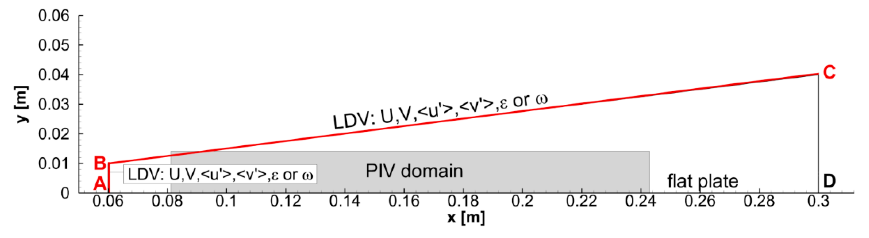
The tuning of the model parameters for transition in separated boundary layer state was completed with selected cases from the experimental data base of Simoni et al. [16] for boundary layer flows on a flat plate. We refer to cases of the data base by the acronym UNIGE, which stands for University of Genoa. The measured flow domain is a trapezoidal area, as shown in Figure 3, bounded by the AB, BC and CD lines. The AB and CD sides of the trapezoid are 10 and 40 mm high, respectively. The AB side is at 60 mm downstream of the leading edge of the plate. The BC side begins at 10 mm above the plate at 60 mm from the leading edge and ends 40 mm above the plate at the plate end (300 mm). Four cases were selected that are representative for separation-induced transition, two cases for bypass transition and two cases with a laminar boundary layer without transition. The cases are listed in

Table 2. Summary of UNIGE test cases. The Reynolds number is based on the plate length and the mean free-stream velocity at the leading edge of the plate. The free-stream turbulence intensity, Tu, is reported at the edge of the boundary layer at the inlet to the computational domain (60 mm downstream of the leading edge of the plate). The numbers 70, 150 and 220 refer to the Reynolds numbers (70k, 150k and 220k). The turbulence levels are coded by LLTU (lowest), LTU (low), HTU (high), HHTU (highest). The adverse pressure gradients are coded by the opening angle of the diverging section of the wind tunnel (0°, 5°, 9° and 12°). The acronym APG stands for adverse pressure gradient.

Test Case	Re	Tu [%]	Pressure Gradient	Transition Mode / Flow
70LLTU12	70,000	1.5	strong APG	separation-induced
70LTU12	70,000	2.5	strong APG	separation-induced
70LTU9	70,000	2.5	moderate APG	separation-induced
70HTU9	70,000	3.5	moderate APG	separation-induced
150LTU5	150,000	2.5	mild APG	bypass
220LTU5	220,000	2.5	mild APG	bypass
70LLTU5	70,000	1.5	mild APG	laminar (no transition)
150LLTU5	150,000	1.5	mild APG	laminar (no transition)

. The free-stream turbulence intensities are categorised in the data base with the terms lowest, low, high and highest, corresponding to 1.5%, 2.5%, 3.5% and 5% at the plate leading edge. The values at the transition point do not differ much. Thus, all turbulence intensities in the data base are actually rather high. With the terminology used here, we categorise the turbulence levels as moderately high to elevated. The adverse pressure gradients in the data base range from zero pressure gradient to a magnitude with a K-value of about three at the point of transition. Thus, the three pressure gradient levels called mild, moderately high and strong in this paper occur. However, the adverse pressure gradient may be stronger in practice. We discuss a case with a stronger adverse pressure gradient in the next section. The focus of the extension of the transition model is not on cases with a very strong adverse pressure gradient combined with a high free-stream turbulence level, because, as explained in Section 5, the transition model functions already for such cases, without the proposed modifications.

The experiments deliver the mean velocity components in the x- and y-directions, the corresponding root mean square velocity fluctuation levels and the integral time-scale of the fluctuations on the inflow boundaries of the computational domain (the AB and BC lines). The mean velocity components were directly imposed on these lines and constant static pressure was imposed on the outlet boundary (CD Line). The inlet profiles of k and ω were derived from the experimental data by the procedures described in Simoni et al. [16]. No-slip conditions were set along the plate, combined with the boundary conditions for k and ω by the Equation (12).

Steady two-dimensional incompressible Navier–Stokes equations were used, discretized by the finite volume method, with second-order upwind approximation of convective fluxes and second-order central representation of diffusive fluxes, available in the ANSYS Fluent CFD-package (version 15). The transition model was implemented by the User Defined Function-facility. The solution of the equations was by the coupled pressure-based algorithm with iterations done until the normalised residuals of the momentum and the transport equations dropped below 10⁻⁶.

A good-quality grid was generated with a structured part near the plate and an unstructured part away from the plate. The total number of cells was 36,000, with values of y⁺ below 0.01 along the plate. A grid sensitivity study was completed with a coarser grid of 25,000 cells, with y⁺ about one along the plate, and a finer grid of 77,000 cells. The shape factor distributions along the plate were visually identical on all meshes (results not shown). The basic mesh was thus proven to be fine enough and it was chosen for the simulations.

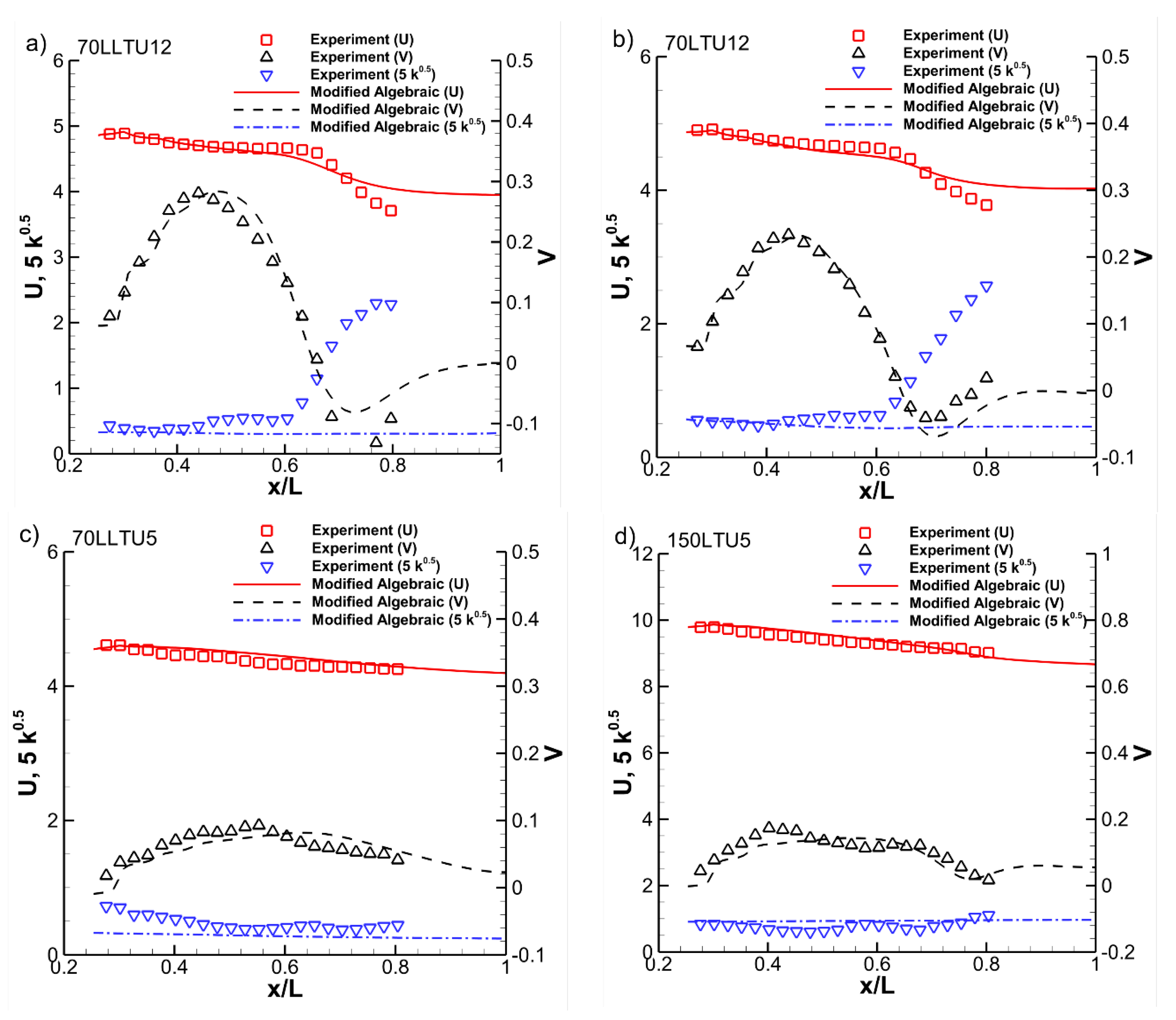
In order to assess the quality of the imposed inlet conditions along the AB and BC lines, a comparison is made in Figure 4 between the mean x- and y-velocity components, and the turbulent kinetic energy, at the distance y/L = 0.04 (12 mm) from the plate, as measured using Particle Image Velocimetry (PIV) and as numerically obtained. The comparison is made for four cases (70LLTU12, 70LTU12, 70LLTU5 and 150LTU5), but a similar level of agreement was obtained with the other four cases. The wall normal distance, y/L = 0.04, is four to five times δ (δ is the boundary layer thickness) at the domain inlet (AB line) and 0.7 to 4 times δ at the domain outlet (CD line). The differences in the boundary layer thickness are due to variability of the Reynolds number, the turbulence level and the pressure gradient. In the cases with bypass transition and the cases with a laminar boundary layer that is prone to separation, the y/L = 0.04 line is above the boundary layer edge on all streamwise positions. In the cases with the strong adverse pressure gradient and boundary layer separation, the y/L = 0.04 line enters the boundary layer on the rear part of the plate.

Figure 4a,b show the comparison between the distributions of measured and predicted x- and y- mean velocity components and turbulent kinetic energy, k, for the cases with strong pressure gradient and separated boundary layer (70LLTU12 and 70LTU12). The agreement is good for x/L < 0.6, but for x/L > 0.6 the numerical k-values are much too low. This is caused by the inability of the steady two-dimensional RANS simulation to reproduce the flow unsteadiness associated with the Kelvin–Helmholtz rolls. So, the difference for x/L > 0.6 is not caused by an error in the inlet conditions. With a laminar boundary layer along the plate (70LLTU5: Figure 4c) and with bypass transition (150LTU5: Figure 4d), the agreement between measured and computed mean velocity components and k-values is good along the whole y/L = 0.04 line.

Four constants determine the f_sep-function. The constants a_γ, b_γ and b_ω are not critical. This is in contrast to the constant a_ω, which has to be chosen so that f_sep does not become active in an attached laminar boundary layer and in the turbulent part of an attached turbulent boundary layer, and that it defines the front part of a separated laminar boundary layer. In order to ensure that the results of the previous version of the model are not changed much in a boundary layer that stays laminar, a sensitivity analysis to the value of a_ω was performed. 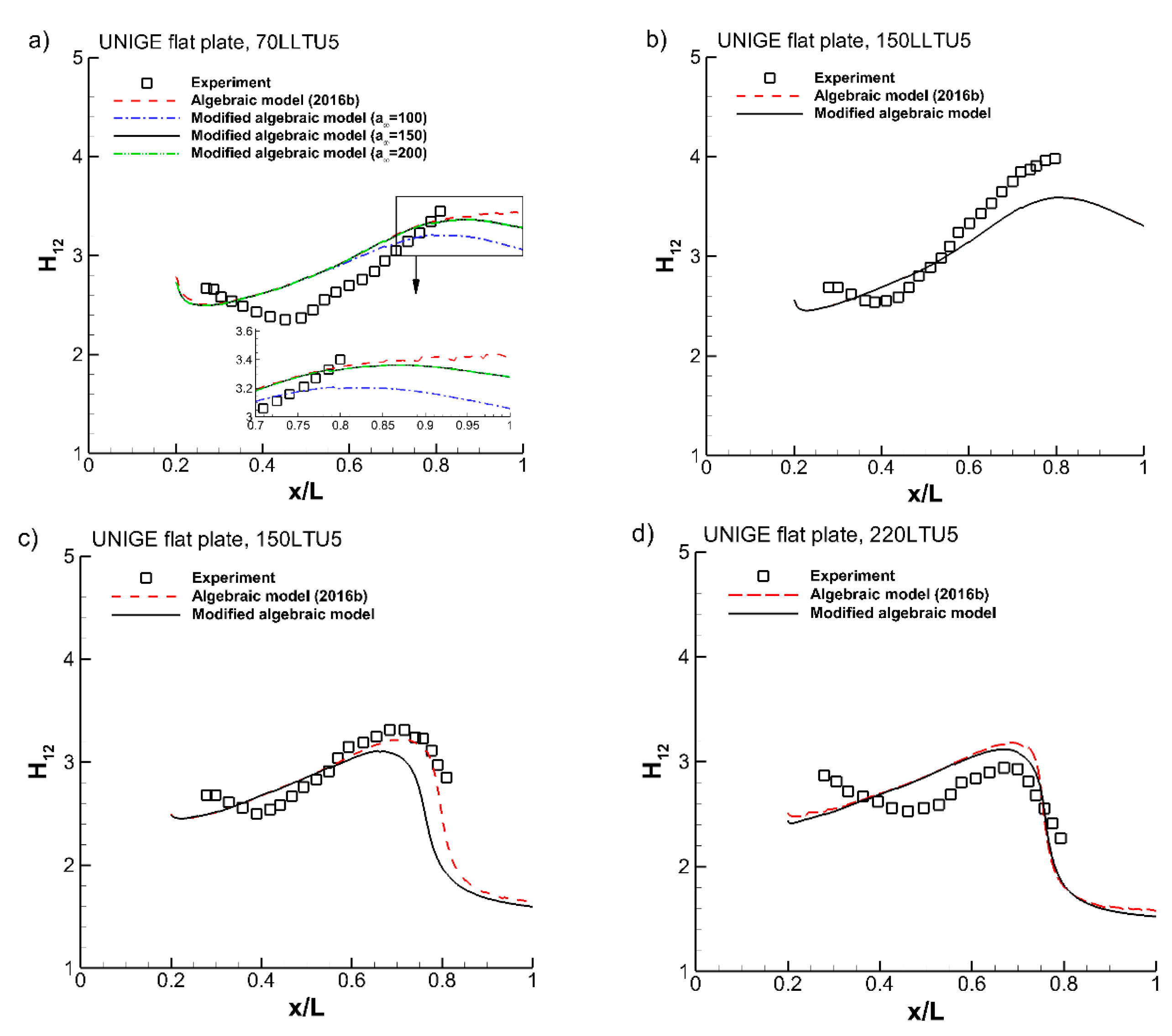Figure 5a shows the shape factor evolution along the plate for the 70LLTU5 case, obtained with the previous model version and with the extended model, using a_ω = 100, 150 and 200. The results produced by the previous model version are quite good. With a_ω = 100 some differences are observed between the results of the two versions. The results are almost unaltered for a_ω = 150 and 200. It means that a_ω = 100 is not high enough. We thus set a_ω = 150. Figure 5b shows the shape factor evolution by the extended model version with a_ω = 150 and the previous version for the second case without transition to turbulence before the end of the plate. No differences are observed between the results of the two model versions, and the results agree well with the experiment.

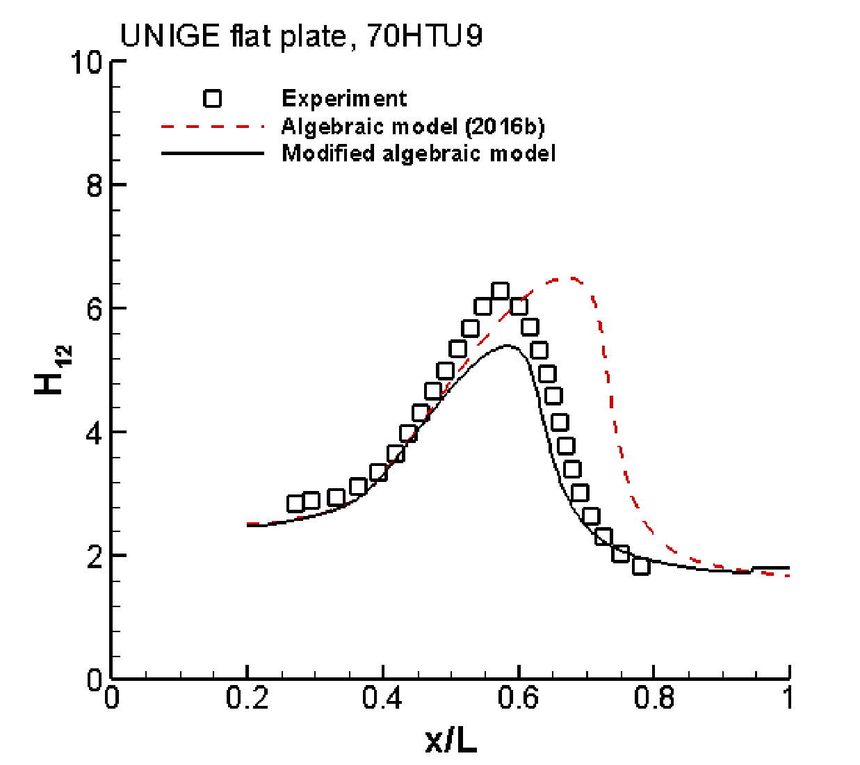
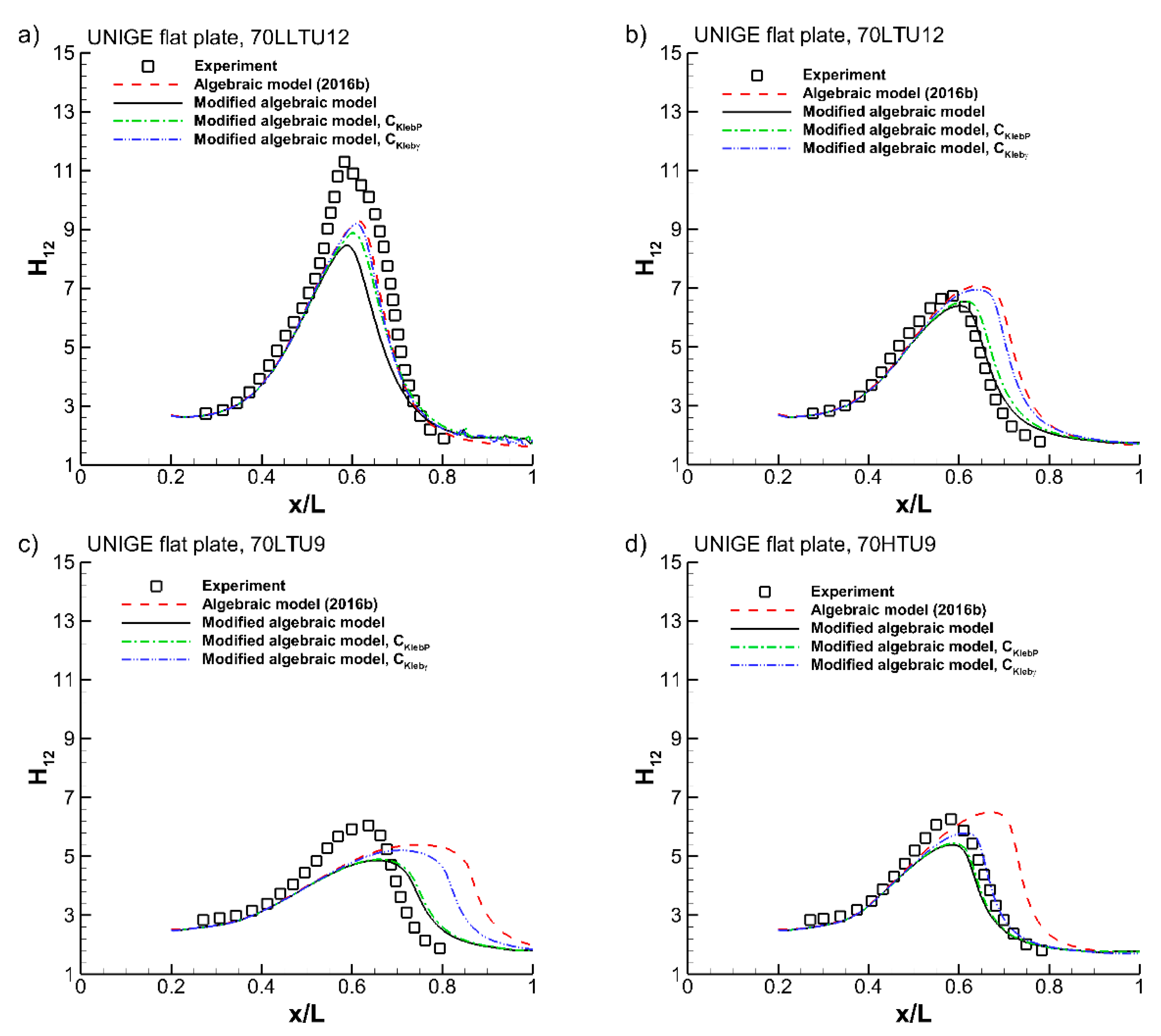
With selected values of the constants a_γ, b_γ, a_ω and b_ω (Equation (11)) and the constant a_Kleb (Equation (13)), the values of C_Klebγ (Equation (7)) and C_KlebP (Equation (8)) have to be tuned. For this purpose, the cases with moderate and strong pressure gradients and a large separation bubble on the plate were used. Figure 6 shows the numerical results for the four cases. The cases are arranged with an increasing turbulence level (a to b and c to d) and decreasing adverse pressure gradient (a and b to c and d). The results by the previous and the modified versions of the algebraic model are represented by the same line types as in Figure 5. In all cases, the supplementary production term in the k-equation (the P_sep-term on r.h.s. of Equation (1)) was active inside the separated boundary layer. This supplementary term triggers the transition in the separated-boundary layer, and further downstream (towards the end of the plate) the main production term (the P_k-term on r.h.s. of Equation (1)) takes over.

Two additional results are represented in Figure 6. The one denoted by C_KlebP is with a deactivated f_sep-term in the intermittency expression (7), (C_Klebγ = 0). The other one denoted by C_Klebγ is with a deactivated f_sep -term in the boosting production P_sep term (8), (C_KlebP = 0). The boosting term based on f_KH is always active (first part of Equation (8)). The effect of the f_sep-term in the expression of the intermittency, when used alone (C_Klebγ), increases in the order of the cases a to d, but cannot be tuned for good results in all four cases. With C_Klebγ = 0.3, the result of the fourth case, which is the one with the highest free-stream turbulence level, becomes good. The f_sep-term in the boosting production term, when used alone (C_KlebP), greatly improves the predictions and can be tuned for good results, albeit not perfect, in all four cases. The tuned value is C_KlebP = 0.01. When both f_sep-terms are active (full black line), the results do not differ much from those with the C_KlebP -term alone. It is thus not possible to accurately tune the value of C_Klebγ, when the C_KlebP-term is already used. However, clearly C_Klebγ = 0.3 is an appropriate value. From Figure 6, we conclude that it is beneficial to add the C_KlebP-term in the boosting production term (Equation (8)). We also conclude that it does not harm to add the C_Klebγ-term in the expression of the intermittency (Equation (7)), but that this addition is not necessary for the cases studied. For completeness, we mention that the results shown in the previous Figure 4 and Figure 5 do not change when the C_Klebγ-term is not used in the expression of the intermittency. Based on the tuning in this section, one may conclude that the C_Klebγ-term is not needed. We maintain it, however, because it allows a somewhat improved prediction for transition in a separated state under a very strong adverse pressure gradient and a high free-stream turbulence level, as we demonstrate in the next section.

All results in Figure 6 have a somewhat too low predicted peak value of the shape factor. This is due, as discussed in Section 5, to production of turbulent kinetic energy by the model in the instability zone of the separated layer, which does not occur in reality. The choice for C_KlebP = 0.01 is a compromise among the four cases shown in Figure 6 for a_Kleb = 1. We mention that comparable results are obtained by a somewhat larger value of C_KlebP together with a somewhat lower value of a_Kleb. However, the best results are obtained by keeping C_KlebP as low as possible, because a larger value of C_KlebP advances the transition prediction of the bypass transition cases (Figure 5c,d), where the influence of the value of a_Kleb is much less.

With the results shown in Figure 5 and Figure 6 in this section, one understands that the role of the added terms in the extended model is rather limited. Without the added terms, the transition model functions already for all transition types, but the added terms improve the predictions for transition in separated state under a moderately strong adverse pressure gradient, in the presence of a moderately high or elevated free-stream turbulence level.

8. Verification of the Model for Transition in Separated State under a Very Strong Adverse Pressure Gradient and a Moderately High Free-Stream Turbulence Level

The pressure gradient parameter expressed by K = −10⁶νU⁻²(dU/dx) is, at most, about three at the position of separation in the cases used for tuning in the previous section. Stronger adverse pressure gradients may occur in practice. Therefore, we verify the model on a case with a much larger adverse pressure gradient, with a K-value of about 4.75 at the position of separation. The free-stream turbulence intensity is moderately high.

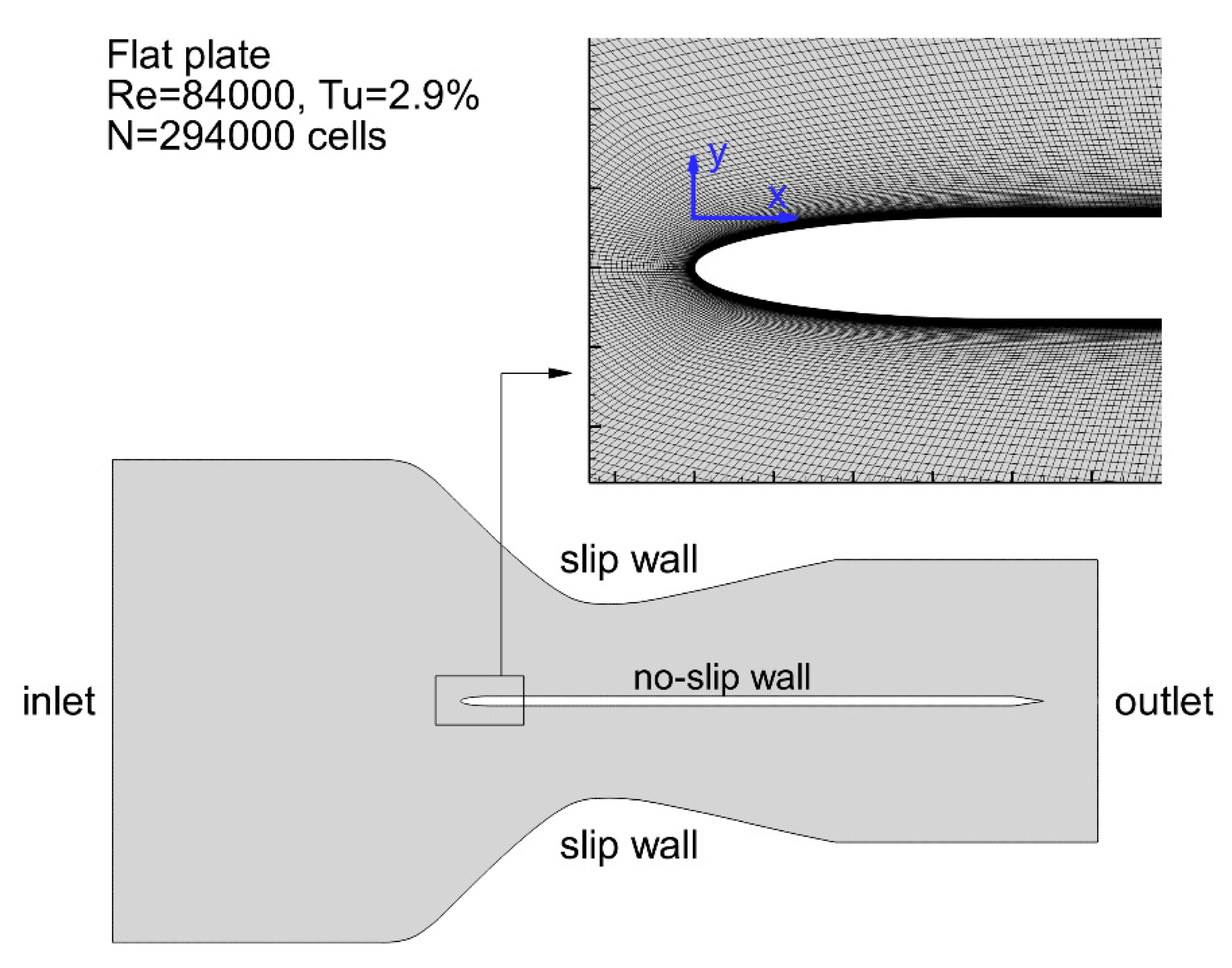
Figure 7 shows the geometry and the boundary conditions for the numerical simulation. The flow over the flat plate was experimentally studied by Coull and Hodson [15] and simulated using LES by Nagabhushana Rao et al. [34] and by Li and Yang [10]. The domain in Figure 7 is a two-dimensional section of the domain used by Li and Yang, with length 1315 mm, inlet height 644 mm and outlet height 377 mm. The length of the test area on the plate is S₀ = 500 mm. The plate thickness is 12.8 mm. The leading edge is elliptical, with a semi-major axis equal to 38 mm. The Reynolds number is 84,000, based on the length S₀ and the mean velocity in the free stream at the end of the test area (S₀ = 500 mm). Slip conditions were applied at the two contoured walls opposite to the plate, no-slip conditions along the plate, and the flow velocity at the inlet was set to U = 1.34 m/s, as in the LES by Li and Yang [10].

The inlet values of the turbulence quantities, k and ω, were obtained by tuning. Both in the experiment (Tu = 3.0%) and the LES by Li and Yang (Tu = 2.9%), the free-stream turbulence intensity at the leading edge of the plate was reported. In addition, the free-stream turbulent length scale at the leading edge was reported in the experiment (l_t = 30.1 mm). The wall-normal distance for the free-stream values of the turbulence level and the turbulent length scale was not specified in the experiment and neither in the LES. The distance y/S₀ = 0.12 was selected by visual inspection of Figure 5 in the work by Coull and Hodson [15]. The inlet values of turbulence level, Tu = 6.5 %, and turbulent length scale, l_t = 22.7 mm, were iteratively determined until the turbulence level, Tu = 2.9%, and the turbulent length scale, l_t = 30.1 mm, were obtained at the plate leading edge.

The same numerical algorithms were employed as in the cases discussed earlier. Iterations were done until the normalised residuals of the momentum and the transport equations dropped below 10⁻⁵. A good quality grid was generated with 294,000 cells and y⁺ < 0.06 along the plate (basic grid). A grid sensitivity study was performed by simulation on a coarser grid with 90,000 cells. The wall shear stress distribution obtained on the coarser grid was the same as that on the basic one. This ensures grid independency of the basic grid results.

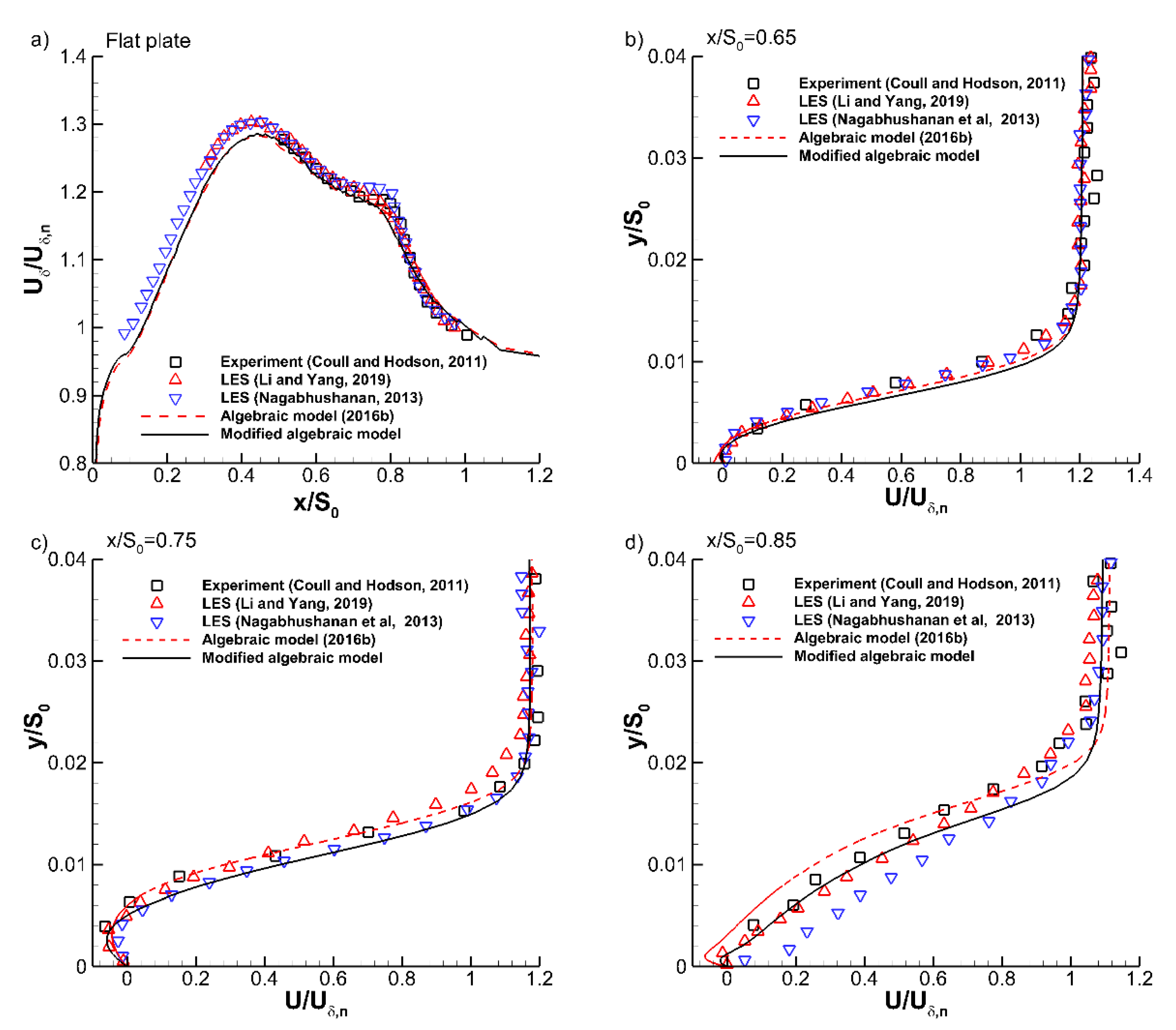
Figure 8a shows the evolution of the mean x-velocity at the boundary layer edge, as measured by Coull and Hodson, [15], simulated using LES by Nagabhushana Rao et al. [34] and by Li and Yang [10], and predicted by both versions of the transition model. The evolution of the edge velocity is correct with both versions of the transition model.

Figure 8b–d shows profiles of the mean x-velocity as a function of the wall-normal distance at the streamwise positions x/S₀ = 0.65, 0.75, and 0.85, obtained by the experiments, by both LES and by two-dimensional RANS with the previous and the extended versions of the transition model. The position x/S₀ = 0.65 is just downstream of the separation point (0.62), while the position x/S₀ = 0.85 is just upstream of the reattachment point (0.87).

The contoured walls were constructed by Nagabhushana Rao et al. and by Li and Yang with the objective to match the free-stream conditions of the experiment by Coull and Hodson. The walls differ slightly and they also differ from the wind tunnel walls of the experiment, which have bleeds for preventing boundary layer separation. Here, we use exactly the same wall and plate shapes as used by Li and Yang. So, we compare the two-dimensional RANS results, with the LES results by Li and Yang. The other results are shown for proving the realism of the simulations by Li and Yang.

Both versions of the transition model produce results that show good agreement with the two LES results and the experiment at the first two locations (Figure 8b,c), where the boundary layer flow is experimentally still laminar. The correspondence with the LES of Li and Yang is somewhat better by the previous model version, however.

At the position x/S₀ = 0.85, thus just before reattachment, the agreement obtained by the modified transition model with the LES results by Li and Yang is very good up to the wall-normal distance y/S₀ = 0.014. The previous model version predicts a somewhat too late reattachment. In the boundary layer edge zone, between y/S₀ = 0.014 and y/S₀ = 0.026, the correspondence with the LES results is less good by both transition model versions. This is not surprising, because the physical unsteadiness, especially at the boundary layer edge, is not captured by the two-dimensional steady RANS simulations.

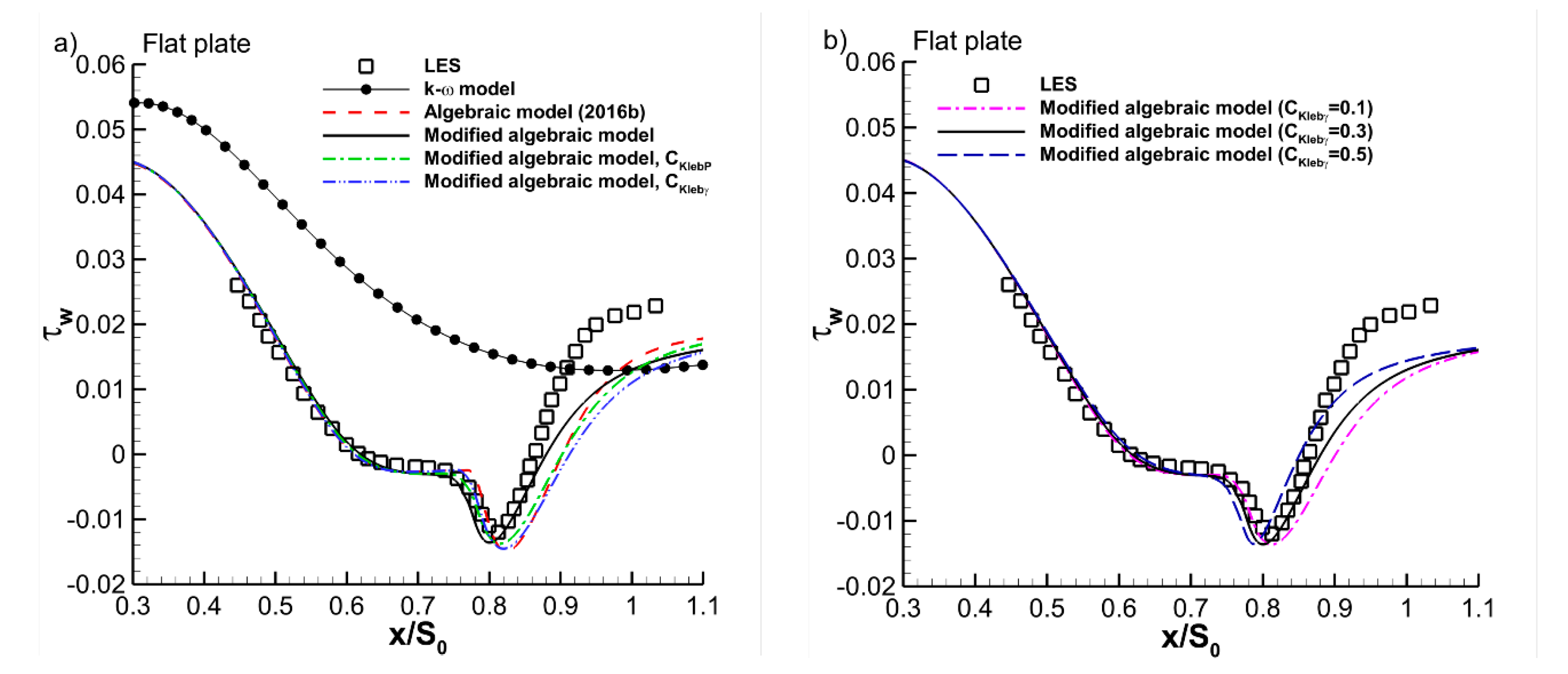
Figure 9a shows the wall shear stress along the plate, obtained by the LES, the fully turbulent k-ω model, and by the k-ω model combined with four versions of the algebraic transition model. With the indications C_Klebγ and C_KlebP is meant that only one of the extensions in the modified model is active (either Equation (7) or Equation (8)). With the reference LES, the separation and reattachment points are at x/S₀ = 0.62 and 0.87. All variants of the algebraic transition model capture well the separation point (x/S₀ = 0.62). The reattachment point is reproduced somewhat too, far downstream, with the previous version of the transition model (x/S₀ = 0.91). An improved result is obtained with the modified model (x/S₀ = 0.88), with both extensions for transition prediction in separated state active. The results with only one of the extensions active, (C_Klebγ or C_KlebP) are near to those of the previous model version. Thus, in this case, the combination of both extensions is necessary for improving the result. The asymptotic behaviour at a large streamwise distance (x/S₀ = 1.1) is not correct with either version of the algebraic transition model, but, clearly this deficiency is caused by the k-ω turbulence model.

The flat plate case studied here is one with a very strong adverse pressure gradient and a moderately high free-stream turbulence level at the position of separation. With such a case, the previous version of the transition model functions already quite well, because the dominant model ingredient is the basic algebraic formula for intermittency (Equation (6)), as explained in Section 5. Nevertheless, an improved prediction is obtained by adding the modifications based on the f_sep-function. Contrary to the cases used for tuning in the previous section, the prediction has now some sensitivity to the value of C_Klebγ, which is illustrated in Figure 9b. The conclusion is that the value C_Klebγ = 0.3, derived in the previous section, is an appropriate value. We repeat that accurate tuning of the value of C_Klebγ is not possible with the data used in the previous section. Clearly, for accurate tuning, a case is needed with separation under a very strong adverse pressure gradient in the presence of a high turbulence level, such that the intermittency (Equation (7)) becomes the dominant ingredient of the transition model.

9. Verification of the Extended Model on Previously Used Cases

It is essential that the terms added to the transition model do not cause loss of quality of the results of the tuning cases of the previous model version. Therefore, verification is demonstrated on some selected cases used in previous work: the four ERCOFTAC (European Research Community on Flow, Turbulence and Combustion) T3C flat plate cases [35], the two flows over the N3-60 turbine vane cascade, measured by Zarzycki and Elsner [36], and the two flows over the V103 compressor blade cascade, simulated with DNS by Zaki et al. [37]. In all cases in this section, the inlet conditions for the mean and fluctuating velocity components, grid resolution and discretisation schemes are the same as in previous work [23,24]. The simulations are completed with steady two-dimensional RANS. We mention that improved results of the V103 compressor cascade were obtained by simulations with three-dimensional unsteady RANS [23].

Table 3. Boundary conditions at the inlet of the computational domain and free-stream turbulence intensity in the leading edge plane for the ERCOFTAC flat plates, the N3-60 and V103 cascades. U denotes the velocity normal to the inlet boundary.

Test Case	U (m/s)	Tu (%)	lt (mm)	TuLE (%)
T3C5	8.95	~3.0	7.0	3.0
T3C2	5.30	~3.0	7.5	3.0
T3C3	3.85	~3.0	9.8	3.0
T3C4	1.25	~3.0	10.4	3.0
N3-60, Tu = 0.4%	8.20	~0.4	2.0	0.4
N3-60, Tu = 3.0%	8.20	~3.0	9.0	3.0
V103, Tu = 3.25%	9.95	3.25	8.0	2.5
V103, Tu = 6.5%	9.95	6.50	5.0	3.9

lists the inlet conditions for the model verification cases and the free-stream turbulence intensity in the leading edge plane.

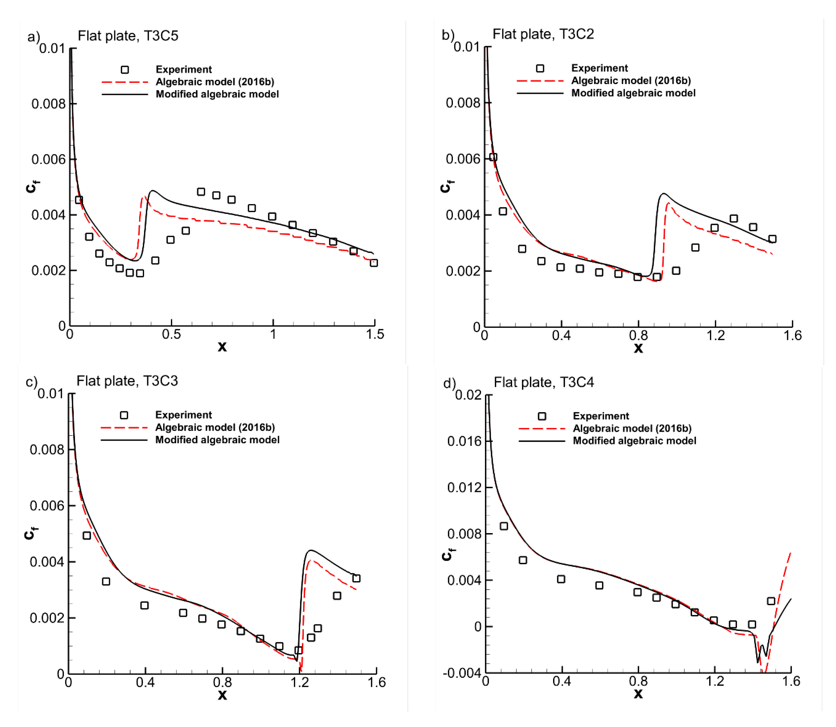
Figure 10 shows the skin friction along the plate for the T3C cases of ERCOFTAC [35]. The wall shear stress is normalised by the local dynamic pressure at the boundary layer edge. The transition is of bypass type in the first three cases. There is a small separation bubble in the fourth case. With the extended model, the evolution of the free-stream turbulence along the plate at the edge of the boundary layer is the same as with the previous model version (not shown). There are small changes in the predicted transition positions. With the bypass cases, the transition zone is always too short, as with the previous model version. This is an inherent feature of the simple algebraic description of the intermittency variable. The extended model produces a better asymptotic behaviour in the turbulent boundary layer region, due to the higher value of the a₂ constant. For the T3C4 case with transition in a separated state (Figure 10d), the experimental skin friction coefficient is represented as zero in the separation bubble. The results by the extended model and the previous model version are almost identical, because the transition is under low free-stream turbulence level and is activated by the f_KH-term, with almost no activity of the f_sep-term. Both model versions predict a somewhat too strong reversed flow in the separation bubble. The conclusion is that the extended model and the previous model version produce comparable results for the ERCOFTAC flat plate cases.

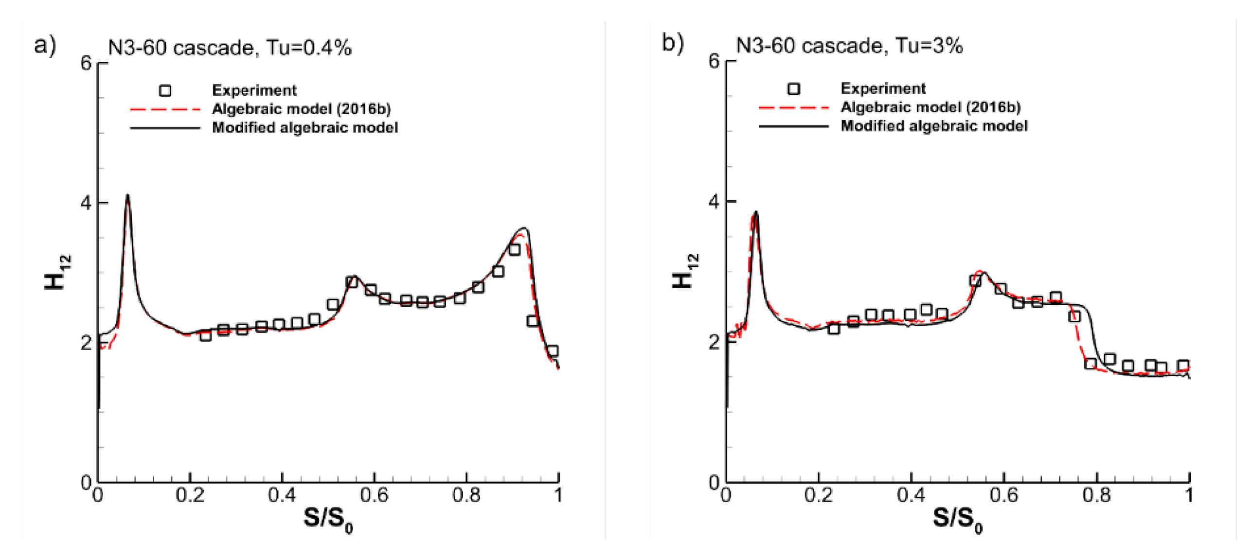
Figure 11 shows the shape factor evolutions along the suction side of the N3-60 turbine vane with low (Tu = 0.4%) and high (Tu = 3%) turbulence levels at the leading edge. The abscissa is the streamwise distance normalised by the surface length, S₀, on the suction side of the blade. The inlet value of the turbulent length scale was not measured in the experiments by Zarzycki and Elsner [36]. For the high turbulence case, the inlet value of the turbulent length scale was adjusted to match the measured turbulence level evolution at the distance 10 mm from the blade suction side [24]. In the low turbulence case, a much smaller value of the turbulent length scale was imposed at the inlet (no grid turbulence in the experiments). In this case (Tu = 0.4%), the results are not sensitive to the precise value of the turbulent length scale. With the previous model version, the agreement with the measurements is good for both cases. With the extended model, the result is identical to that by the previous model version for the low turbulence case (Figure 11a) with transition in separated state. The reason is the same as for the T3C4 flat plate, i.e., that the transition is under low free-stream turbulence level and is activated by the f_KH-term, with almost no activity of the f_sep-terms. There is a small delay of the transition onset prediction by the extended model in the high turbulence case (Figure 11b) with bypass transition. So, as with the flat plate bypass cases T3C5, T3C2 and T3C3, there is a small change in the predicted transition position.

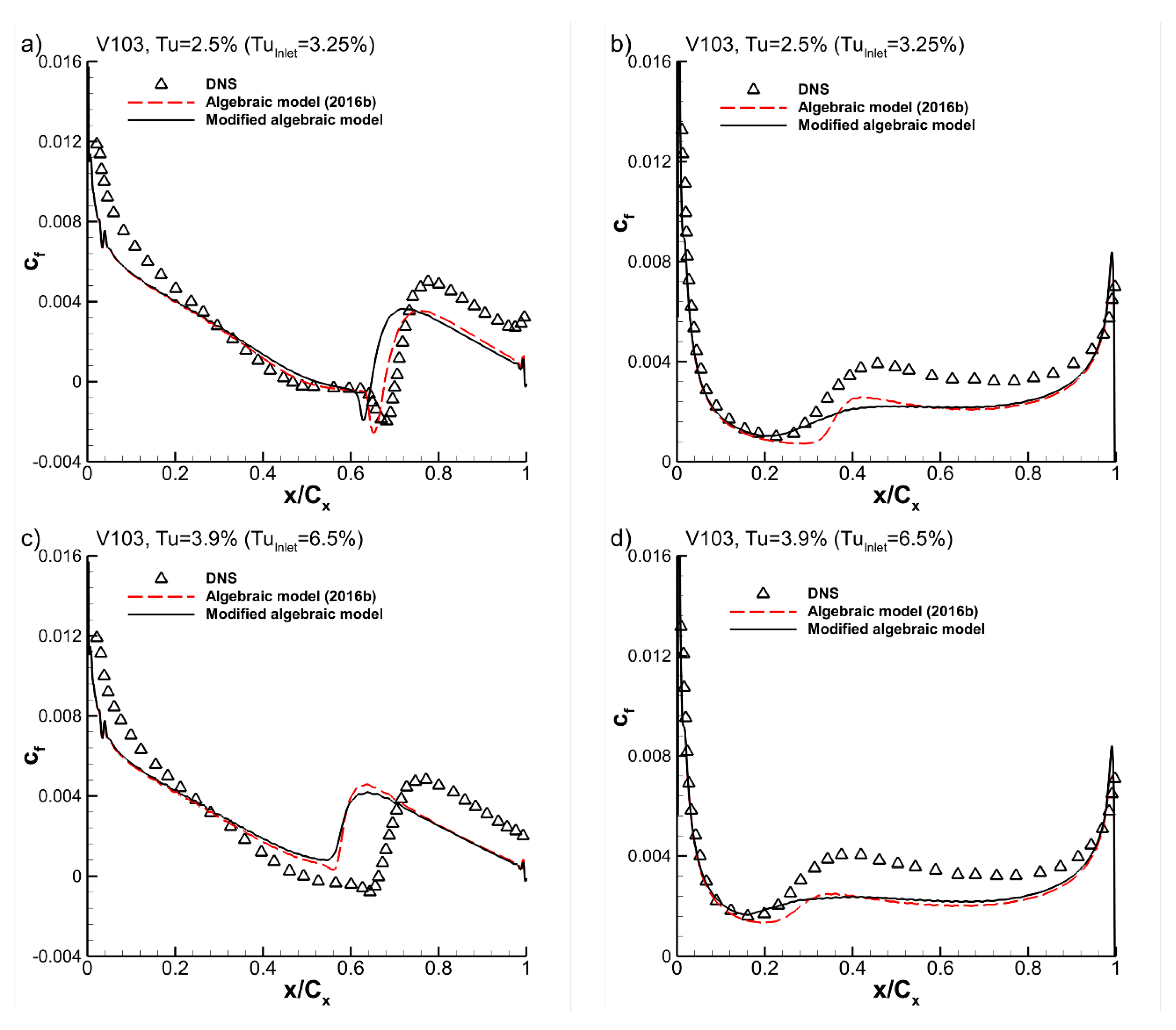
Figure 12 shows the skin friction distributions on the surfaces of the V103 compressor blade with high (Tu = 3.25%) and very high (Tu = 6.5%) free-stream turbulence levels at the inlet of the computational domain, placed 40 % of the axial chord upstream of the cascade leading edge line. The turbulence levels at the leading edge are Tu = 2.5% and 3.9% and are thus quite high. Good matching was obtained of the evolution of the free-stream turbulence level at mid-span with the DNS data [24] (not shown). The flow is subjected to a very strong adverse pressure gradient, with a K-value of about four, on the blade suction side, from 20% of the blade chord on. This causes boundary layer separation, despite the high level of free-stream turbulence. Both transition model versions properly predict the quite large size of the separation bubble for Tu = 2.5% (Figure 12a). The predicted transition positions are near to each other on the suction side with both model versions for both turbulence levels (Figure 12a,c). The explanation is that the modelled transition is by the basic intermittency term for bypass transition (Equation (6)), which functions here for transition in a separated state under a high free-stream turbulence level, as explained in Section 5. There is almost no activity by the f_sep-terms. Both models produce a comparable level of agreement with the DNS results obtained by Zaki et al. [37] on the pressure side of the blade (Figure 12b,d), where the transition is of bypass type. The asymptotic behaviour in the turbulent boundary layer region is not correct by both transition models, caused by underprediction of the skin friction by the k-ω turbulence model, also present on the suction side (Figure 12a,c) in fully turbulent flow.

10. Conclusions

A modified algebraic intermittency model has been developed, which improves predictions of RANS simulations by the previous model version [24], for separation-induced transition under a moderately high or elevated turbulence level. Two extensions have been made in the production term of the equation for turbulent kinetic energy of a k-ω turbulence model. The extensions express the effect of Klebanoff streaks generated upstream of separation on the splitting in the separated part of the layer of full-span Kelvin–Helmholtz instability rolls into part-span structures, which accelerates the breakdown, and the direct effect of the Klebanoff streaks on the breakdown of the separated layer. By the Klebanoff streaks, the breakdown is faster and occurs under the combined effects of a large adverse pressure gradient and a large free-stream turbulence level. The algebraic intermittency model is a simple alternative for commonly used transition models with transport equations for simulation of turbomachinery flows.