Impact of Underlying RANS Turbulence Models in Zonal Detached Eddy Simulation: Application to a Compressor Rotor

Abstract
1. Introduction
2. Experimental Facility
3. Numerical Test Bench
4. Zonal Detached Eddy Simulation
5. Rotor Performances
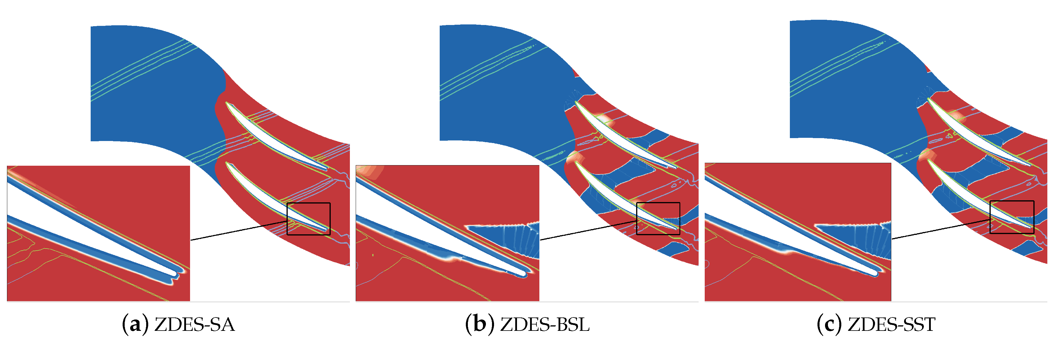
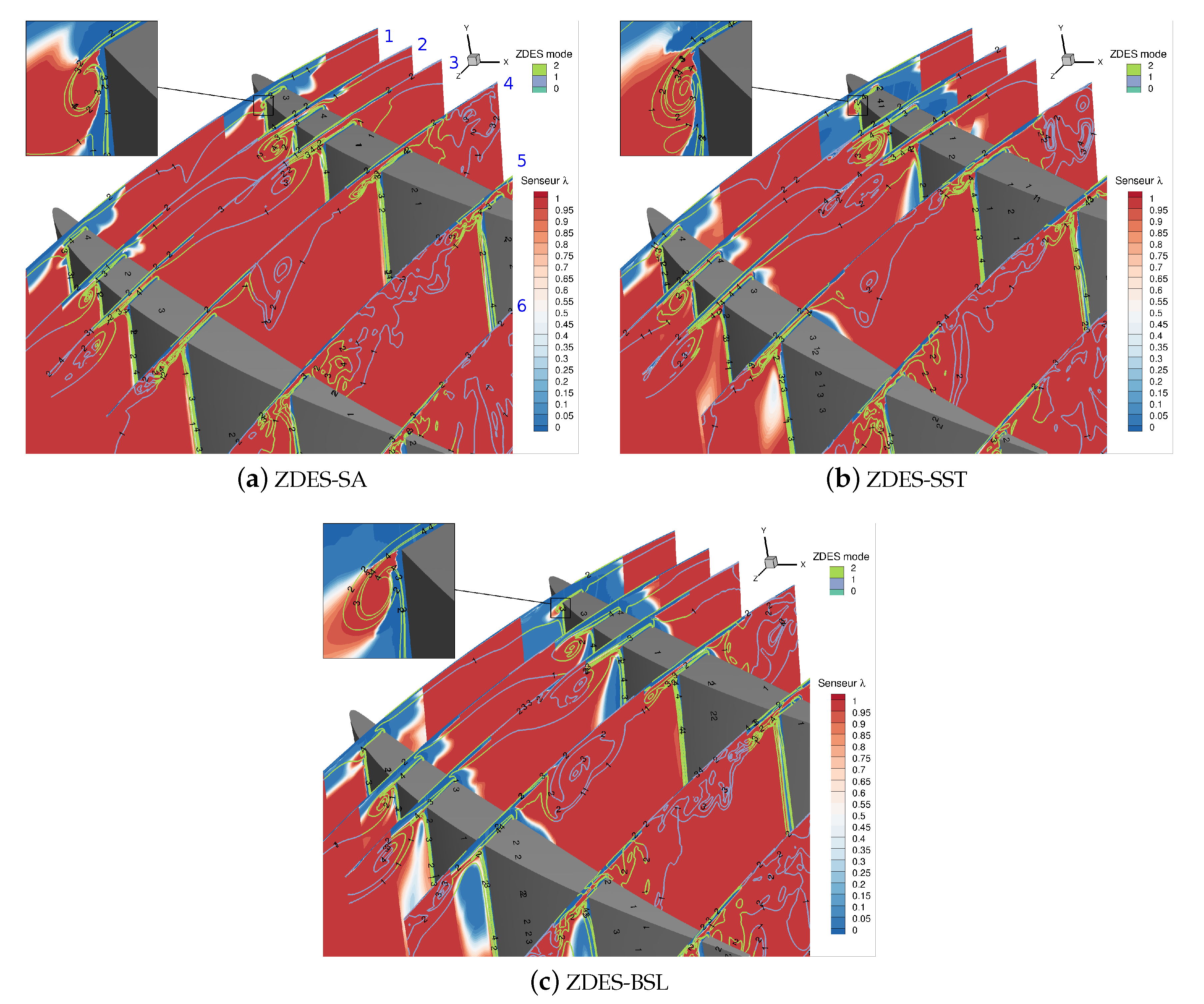
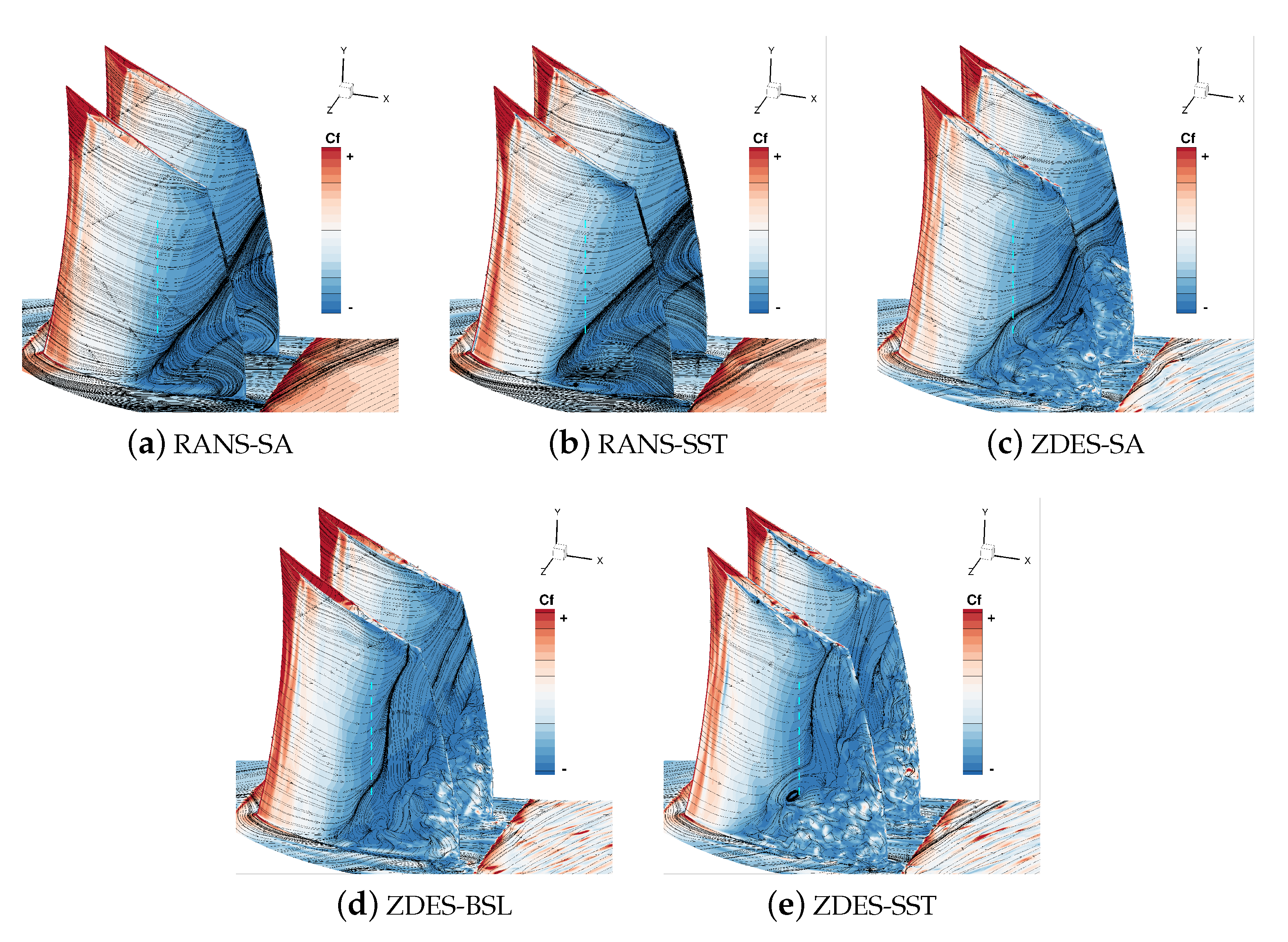
6. Flow around Rotor Blades
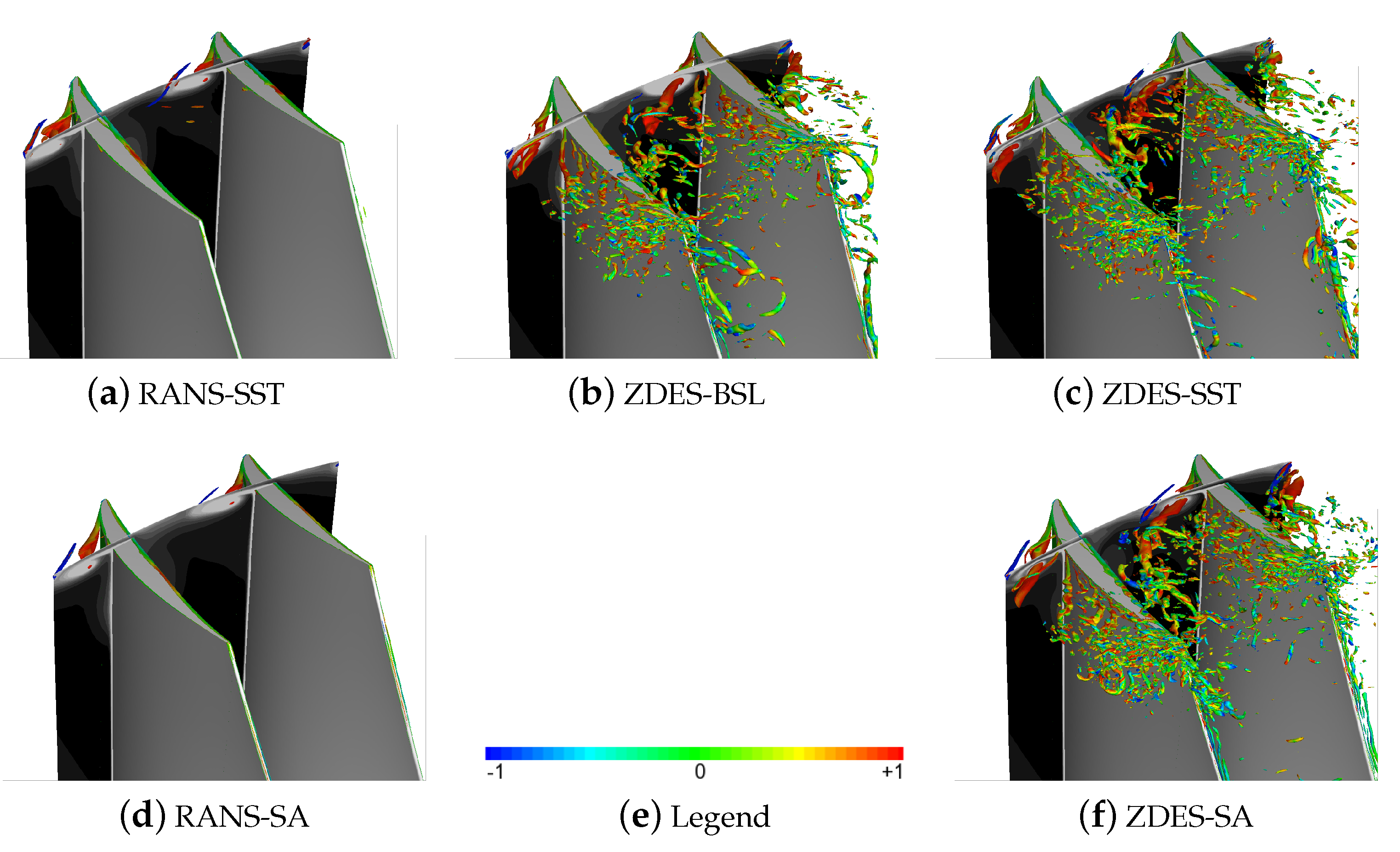
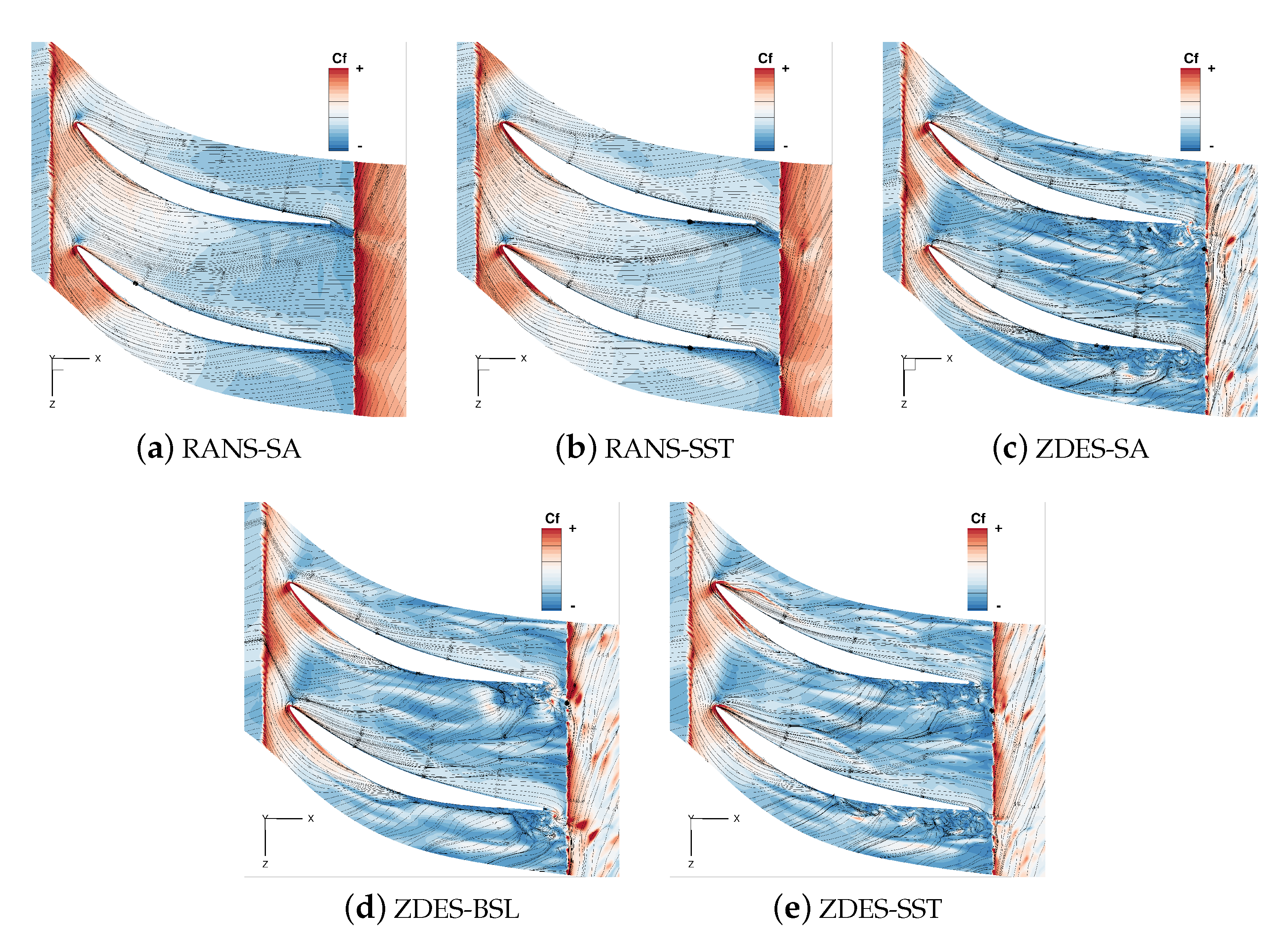
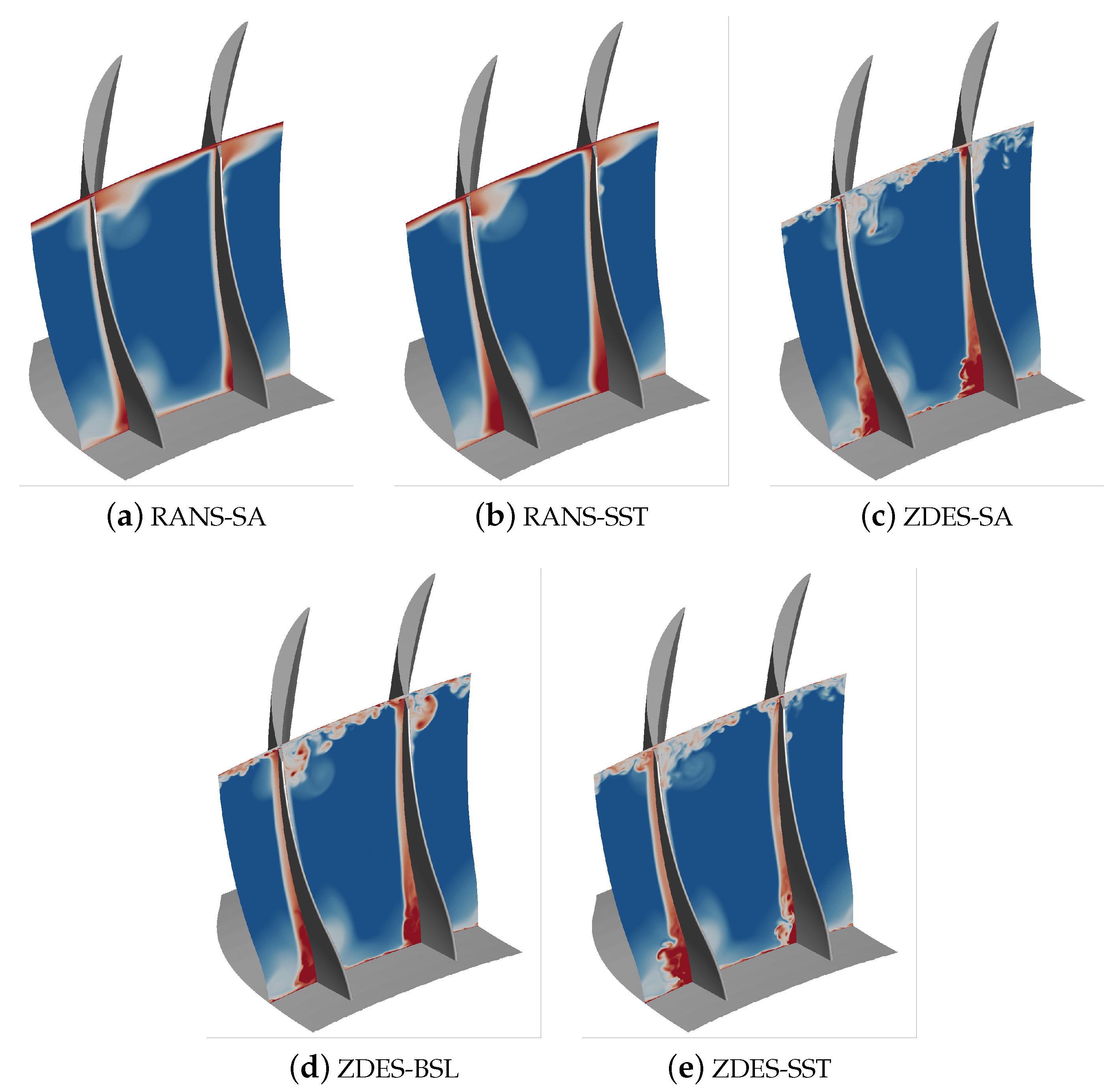
7. Tip Leakage Flow
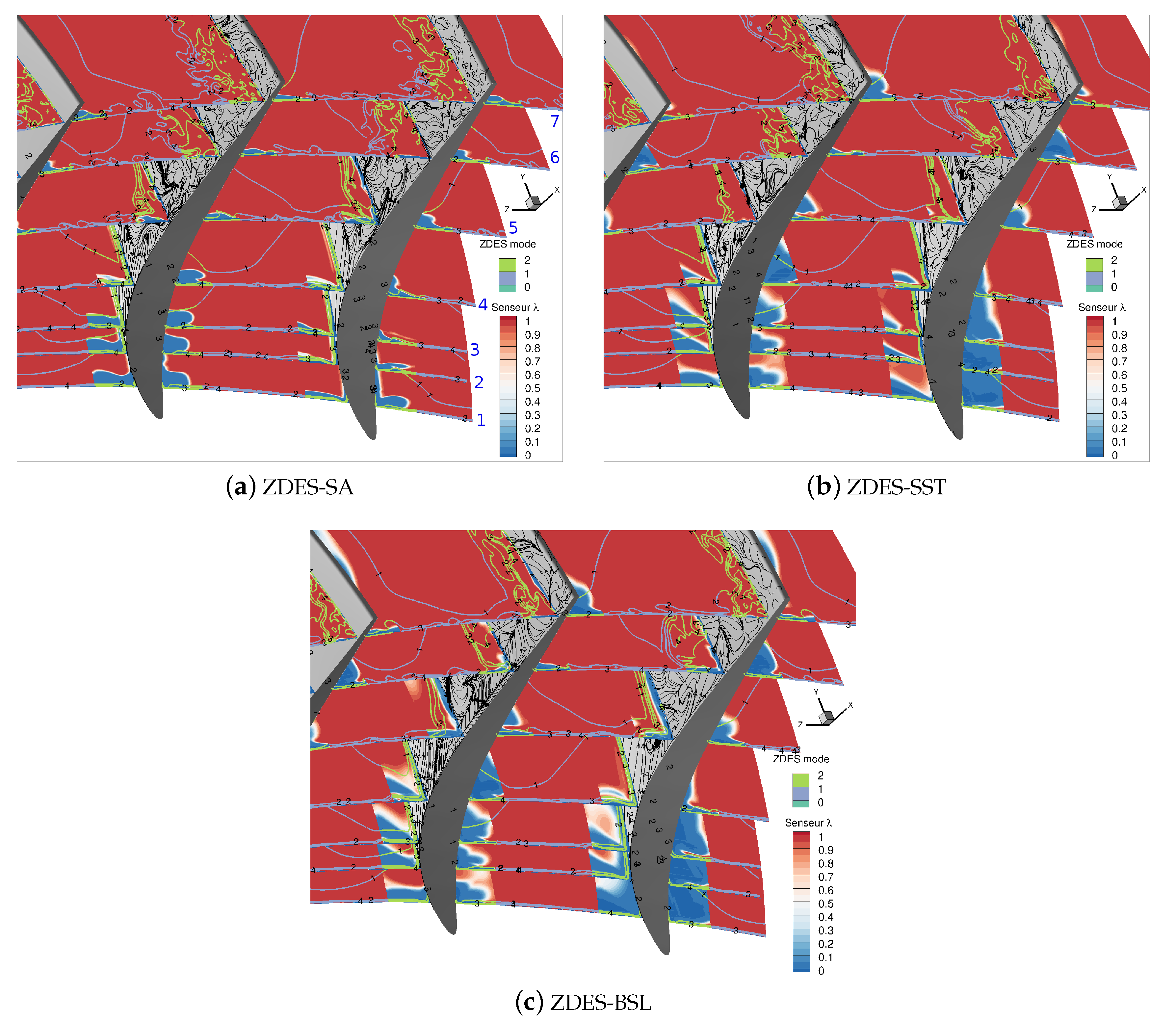
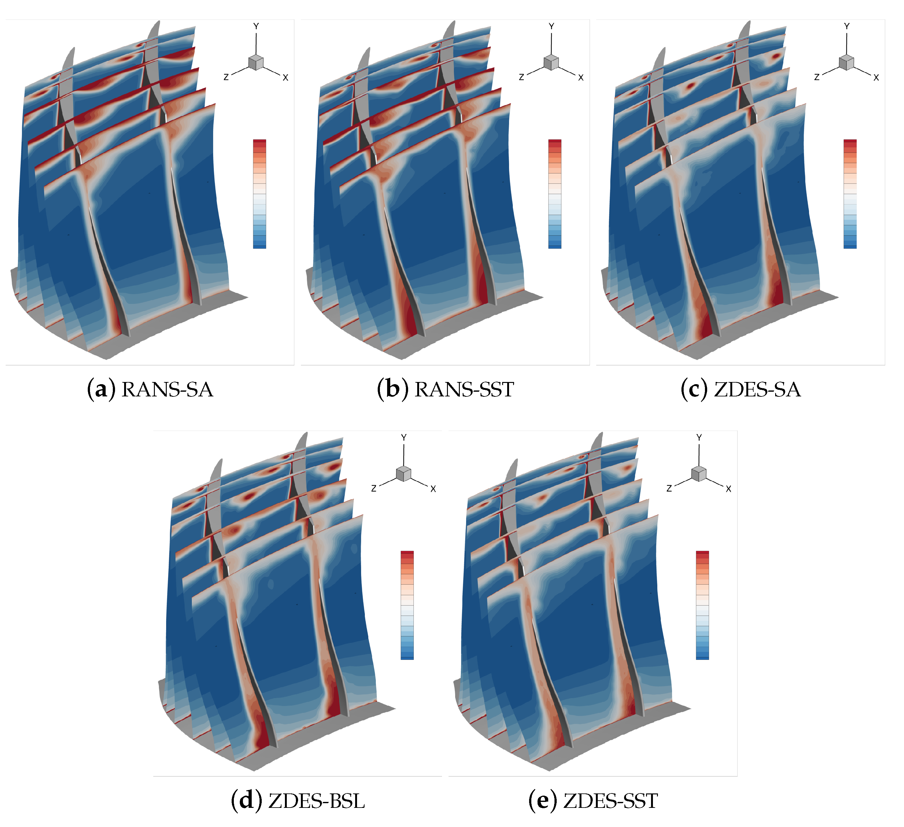
8. Hub Corner Flow
9. Conclusions
Author Contributions
Funding
Acknowledgments
Conflicts of Interest
Abbreviations
| BSL | BaSeLine Menter turbulence model |
| HRLES | Hybrid RANS/LES |
| IGV | Inlet Guide Vane |
| LDA | Laser Doppler Anemometry |
| LES | Large Eddy Simulation |
| R1 | First rotor of CREATE compressor |
| RANS | Steady/unsteady Reynolds-Averaged Navier–Stokes |
| SA | Spalart–Allmaras turbulence model |
| SST | Menter turbulence model with SST correction |
| ZDES | Zonal Detached Eddy Simulation |
References
- Greitzer, E.; Tan, C.; Graf, M. Internal Flow: Concepts and Applications; Cambridge Engine Technology Series; Cambridge University Press: Cambridge, UK, 2007. [Google Scholar]
- Denton, J. Loss Mechanisms in Turbomachines. J. Turbomach. 1993, 115, 621–656. [Google Scholar] [CrossRef]
- Mailach, R.; Lehmann, I.; Vogeler, K. Rotating Instabilities in an Axial Compressor Originating From the Fluctuating Blade Tip Vortex. J. Turbomach. 2000, 123, 453–460. [Google Scholar] [CrossRef]
- Margalida, G.; Joseph, P.; Roussette, O.; Dazin, A. Comparison and Sensibility Analysis of Warning Parameters for Rotating Stall Detection in an Axial Compressor. Int. J. Turbomach. Propuls. Power 2020, 5, 16. [Google Scholar] [CrossRef]
- Courtiade, N.; Ottavy, X. Experimental Study of Surge Precursors in a High-Speed Multistage Compressor. J. Turbomach. 2013, 135, 061018. [Google Scholar] [CrossRef]
- Thiam, A.H.; Whittlesey, R.W.; Wark, C.E.; Williams, D.R. Corner Separation and the onset of stall in an axial compressor. In Proceedings of the 38th Fluid Dynamics Conference and Exhibit, Seattle, WA, USA, 23–26 June 2008. [Google Scholar] [CrossRef]
- Tyacke, J.; Tucker, P.G.; Jefferson-Loveday, R.; Vadlamani, N.R.; Watson, R.; Naqavi, I.; Yang, X. Large Eddy Simulation for turbines: Methodologies, cost and future outlooks. J. Turbomach. 2013, 136, 061009. [Google Scholar] [CrossRef]
- McMullan, W.; Page, G. Towards Large Eddy Simulation of gas turbine compressors. Prog. Aerosp. Sci. 2012, 52, 30–47. [Google Scholar] [CrossRef]
- Chapman, D.K. Computational Aerodynamics Development and Outlook. AIAA J. 1979, 17, 1293–1313. [Google Scholar] [CrossRef]
- Tyacke, J.; Tucker, P. Future Use of Large Eddy Simulation in Aeroengines. In Proceedings of the ASME Turbo Expo, Düsseldorf, Germany, 16–20 June 2014. [Google Scholar] [CrossRef]
- Tucker, P.; Eastwood, S.; Klostermeier, C.; Xia, H.; Ray, P.; Tyacke, J.; Dawes, W. Hybrid LES Approach for Practical Turbomachinery Flows—Part I: Hierarchy and Example Simulations. J. Turbomach. 2012, 134, 1–10. [Google Scholar] [CrossRef]
- Tucker, P.; Eastwood, S.; Klostermeier, C.; Xia, H.; Ray, P.; Tyacke, J.; Dawes, W. Hybrid LES Approach for Practical Turbomachinery Flows—Part II: Further Applications. J. Turbomach. 2012, 134, 1–10. [Google Scholar] [CrossRef]
- Spalart, P. Comments on the Feasibility of LES for Wings, and on Hybrid RANS/LES Approach. In Proceedings of the First, AFOSR International Conference on DNS/LES, Ruston, LA, USA, 4–8 August 1997. [Google Scholar]
- Hodara, J.; Smith, M.J. Hybrid Reynolds-Averaged Navier–Stokes/Large-Eddy Simulation Closure for Separated Transitional Flows. AIAA J. 2017. [Google Scholar] [CrossRef]
- Quéméré, P.; Sagaut, P. Zonal multi-domain RANS/LES simulations of turbulent flows. Int. J. Numer. Methods Fluids 2002, 40, 903–925. [Google Scholar] [CrossRef]
- Deck, S. Recent Improvements in the Zonal Detached Eddy Simulation (ZDES) Formulation. Theor. Comput. Fluid Dyn. 2012, 26, 523–550. [Google Scholar] [CrossRef]
- Boudet, J.; Caro, J.; Li, B.; Jondeau, E.; Jacob, M.C. Zonal large-eddy simulation of a tip leakage flow. Int. J. Aeroacoustics 2016, 15, 646–661. [Google Scholar] [CrossRef]
- Su, X.; Ren, X.; Li, X.; Gu, C. Unsteadiness of Tip Leakage Flow in the Detached-Eddy Simulation on a Transonic Rotor with Vortex Breakdown Phenomenon. Energies 2019, 12, 954. [Google Scholar] [CrossRef]
- Liu, Y.; Zhong, L.; Lu, L. Comparison of DDES and URANS for Unsteady Tip Leakage Flow in an Axial Compressor Rotor. J. Fluids Eng. 2019, 141. [Google Scholar] [CrossRef]
- Li, R.; Gao, L.; Ma, C.; Lin, S.; Zhao, L. Corner separation dynamics in a high-speed compressor cascade based on detached-eddy simulation. Aerosp. Sci. Technol. 2020, 99, 105730. [Google Scholar] [CrossRef]
- Riéra, W.; Marty, J.; Castillon, L.; Deck, S. Zonal Detached-Eddy Simulation Applied to the Tip-Clearance Flow in an Axial Compressor. AIAA Journal 2016, 54, 1–15. [Google Scholar] [CrossRef]
- Mockett, C. A Comprehensive Study of Detached-Eddy Simulation. Ph.D. Thesis, Technische Universit, Berlin, Germany, 2009. [Google Scholar] [CrossRef]
- Uribe, C.; Marty, J.; Gerolymos, G. Zonal Detached Eddy Simulation extension to k-ω models. In Proceedings of the 23rd AIAA Computational Fluid Dynamics Conference, Denver, CO, USA, 5–9 June 2017; p. 4279. [Google Scholar] [CrossRef]
- Spalart, P.; Allmaras, S. A one-equation turbulence model for aerodynamic flows. La Recherche Aérospatiale 1994, 1, 5–21. [Google Scholar]
- Menter, F. Two-Equation Eddy-Viscosity Turbulence Models for Engineering Applications. AIAA J. 1994, 32, 1598–1605. [Google Scholar] [CrossRef]
- Ottavy, X.; Courtiade, N.; Gourdain, N. Experimental and Computational Methods for Flow Investigation in High-Speed Multistage Compressor. J. Propuls. Power 2012, 28, 1141–1155. [Google Scholar] [CrossRef]
- Mersinligil, M.; Brouckaert, J.F.; Courtiade, N.; Ottavy, X. A High Temperature High Bandwidth Fast Response Total Pressure Probe for Measurements in a Multistage Axial Compressor. J. Eng. Gas Turbines Power 2012, 134, 11. [Google Scholar] [CrossRef]
- Riéra, W. Evaluation of the ZDES Method on an Axial Compressor: Analysis of the Effects of Upstream Wake and Throttle on the Tip-Leakage Flow. Ph.D. Thesis, École Centrale de Lyon, Écully, France, 2014. [Google Scholar]
- Cambier, L.; Heib, S.; Plot, S. The Onera elsA CFD software: Input from research and feedback from industry. Mech. Ind. 2013, 14, 159–174. [Google Scholar] [CrossRef]
- Mary, I.; Sagaut, P.; Deville, M. An algorithm for low mach number unsteady flows. Comput. Fluids 2000, 29, 119–147. [Google Scholar] [CrossRef]
- Spalart, P.; Deck, S.; Shur, M.; Squires, K.; Strelets, M.; Travin, A. A new version of detached-eddy simulation, resistant to ambiguous grid densities. Theor. Comput. Fluid Dyn. 2006, 20, 181–195. [Google Scholar] [CrossRef]
- Smagorinsky, J. General circulation experiments with the primitive equations: I. The basic experiment. Mon. Weather Rev. 1963, 91, 99–164. [Google Scholar] [CrossRef]
- Deck, S.; Laraufie, R. Numerical investigation of the flow dynamics past a three-element aerofoil. J. Fluid Mech. 2013, 732, 401–444. [Google Scholar] [CrossRef]
- Strelets, M. Detached Eddy Simulation of Massively Separated Flows. In Proceedings of the 39th AIAA Fluid Dynamics Conference and Exhibit, Reno, NV, USA, 8–11 January 2001; pp. 1–18. [Google Scholar] [CrossRef]
- Chauvet, N.; Deck, S.; Jacquin, L. Zonal Detached Eddy Simulation of a Controlled Propulsive Jet. AIAA J. 2007, 45, 2458–2473. [Google Scholar] [CrossRef]
- Shur, M.; Spalart, P.; Strelets, M.; Travin, A. Detached-eddy simulation of an airfoil at high angle of attack. In Engineering Turbulence Modelling and Experiments 4; Rodi, W., Laurence, D., Eds.; Elsevier Science Ltd: Oxford, UK, 1999; pp. 669–678. [Google Scholar] [CrossRef]
- Délery, J.M. Robert Legendre and Henri Werlé: Toward the Elucidation of Three-Dimensional Separation. Annu. Rev. Fluid Mech. 2001, 33, 129–154. [Google Scholar] [CrossRef]
- Zambonini, G.; Ottavy, X.; Kriegseis, J. Corner Separation Dynamics in a Linear Compressor Cascade. J. Fluids Eng. 2017, 139. [Google Scholar] [CrossRef]


| Row | IGV | R1 | S1 | R2 | S2 | R3 | S3 |
|---|---|---|---|---|---|---|---|
| Blade number | 32 | 64 | 96 | 80 | 112 | 80 | 128 |
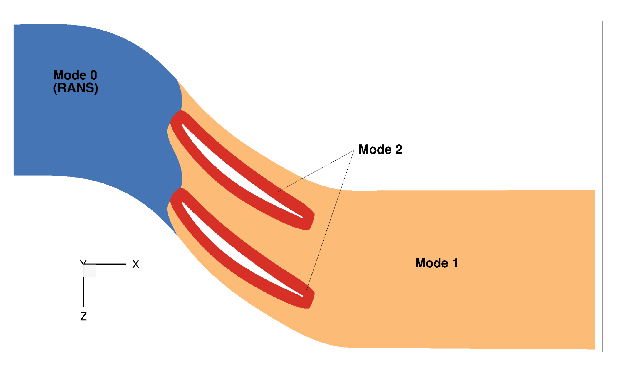
| ZDES SA | ZDES BSL and ZDES SST | |
|---|---|---|
| Substitution of by in terms | ||
| 0.65 | ||
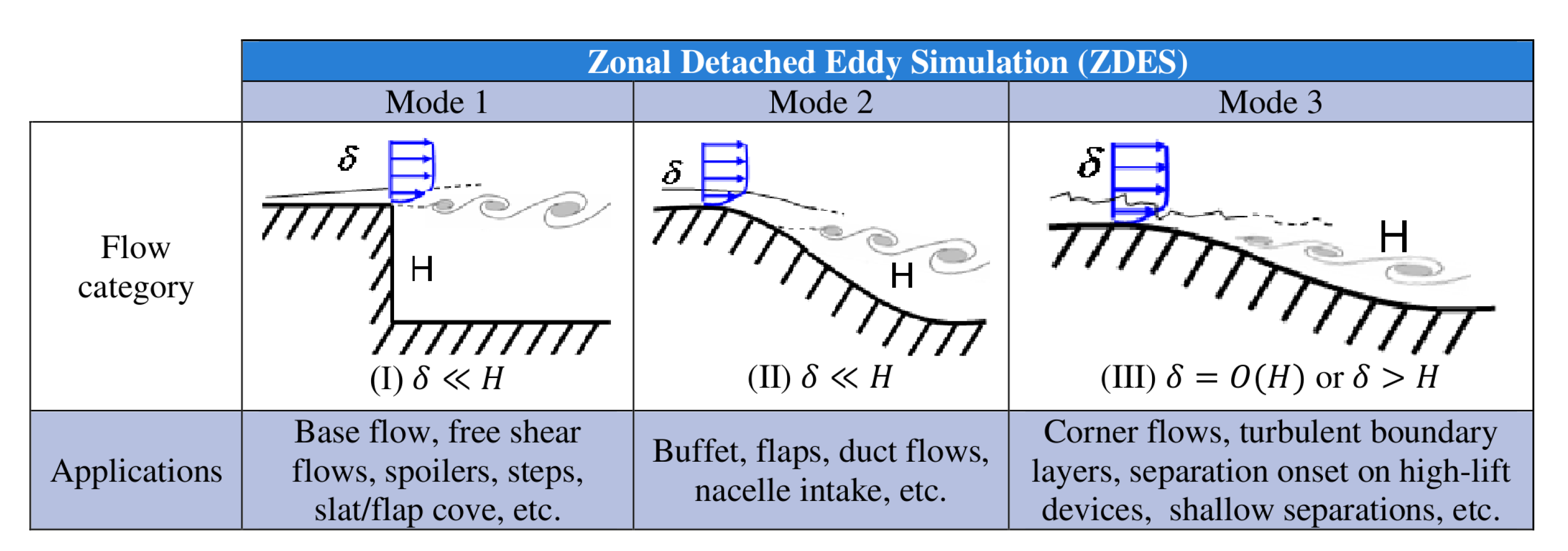
| Mode 1 | ||
| Mode 2 | ||
| 0.8 | 0.8 | |
© 2020 by the authors. Licensee MDPI, Basel, Switzerland. This article is an open access article distributed under the terms and conditions of the Creative Commons Attribution (CC BY) license (http://creativecommons.org/licenses/by/4.0/).
Share and Cite
Marty, J.; Uribe, C. Impact of Underlying RANS Turbulence Models in Zonal Detached Eddy Simulation: Application to a Compressor Rotor. Int. J. Turbomach. Propuls. Power 2020, 5, 22. https://doi.org/10.3390/ijtpp5030022
Marty J, Uribe C. Impact of Underlying RANS Turbulence Models in Zonal Detached Eddy Simulation: Application to a Compressor Rotor. International Journal of Turbomachinery, Propulsion and Power. 2020; 5(3):22. https://doi.org/10.3390/ijtpp5030022
Chicago/Turabian StyleMarty, Julien, and Cédric Uribe. 2020. "Impact of Underlying RANS Turbulence Models in Zonal Detached Eddy Simulation: Application to a Compressor Rotor" International Journal of Turbomachinery, Propulsion and Power 5, no. 3: 22. https://doi.org/10.3390/ijtpp5030022
APA StyleMarty, J., & Uribe, C. (2020). Impact of Underlying RANS Turbulence Models in Zonal Detached Eddy Simulation: Application to a Compressor Rotor. International Journal of Turbomachinery, Propulsion and Power, 5(3), 22. https://doi.org/10.3390/ijtpp5030022