Abstract
A turbocharger’s radial turbine has a strong impact on the fuel consumption and transient response of internal combustion engines. This paper summarizes the efforts to design a new radial turbine aiming at high efficiency and low inertia by applying two different optimization techniques to a parametrized CAD model. The first workflow wraps 3D fluid and solid simulations within a meta-model assisted genetic algorithm to find an efficient turbine subjected to several constraints. In the next step, the chosen turbine is re-parametrized and fed into the second workflow which makes use of a gradient projection algorithm to further fine-tune the design. This requires the computation of gradients with respect to the CAD parametrization, which is done by calculating and combining surface sensitivities and design velocities. Both methods are applied successfully, i.e., the first delivers a well-performing turbine, which, by the second method, is further improved by 0.34% in efficiency.
1. Introduction
The stationary and transient performance of large combustion engines is coined by the design of its turbocharger system, i.e., its compressor and turbine. In the present paper, a radial turbine is designed with a focus on both engine efficiency and transient response. These goals are directly linked to the turbine efficiency and its inertia. Furthermore, a high life expectancy is requested, which constrains the stress levels.
This problem is tackled with two different, subsequent design steps: The first is a gradient-free multidisciplinary optimization based on a meta-model assisted evolutionary algorithm. It can be considered standard in the sense that there are numerous publications that use comparable methods to improve rotor designs, see [1,2,3] or [4]. This method can explore the design space. However, its success is limited as the calculation effort scales with the number of design parameters, i.e., increasing the design space or, respectively, the potential for improvement comes with a great computational cost.
To overcome this major drawback, the global optimization in the first step with a gradient-based optimization in a second step. Additionally, the gradients in the second step are computed following an adjoint technique, which has the advantage that the effort per iteration does not scale with the number of parameters and promises fast design improvements. However, differentiating every available cost function with high accuracy and subsuming all of them in a single optimization is challenging—which is probably why only few authors have presented comparable multidisciplinary design chains. However, there are some, and the potential for design improvements has proven to be considerable, see [5] or [6]. Setting up a multidisciplinary gradient-based design chain, one faces several difficulties. First, the designer needs to have tools available that can calculate mesh sensitivities for the considered cost functions. By now, several open-source and commercial CFD codes are available that offer methods to calculate the flow-related ones using adjoint methods. However, finding codes that can do this for the rest of the considered cost functions (eigenfrequency, mass, inertia) proves troublesome. Hence, in this paper, we apply a combination of commercial codes, open-source academic codes as well as in-house developed programs. Second, one needs to find a way to calculate design velocities, which is compatible with the CAD tool in which the turbine is parametrized. Within this work, a finite difference approach is applied to achieve this. Third, data must be mapped in between meshes, so interpolation methods need to be applied, such as the implemented nearest neighbor algorithm in the presented workflow. Finally, an optimizer is required that handles the different tools and steers the overall process, like the in-house implementation of the gradient projection algorithm according to [7].
In the following, both optimization methodologies will be presented: In the next chapter, the gradient-free framework is detailed, and a turbine is designed. In the subsequent chapter, this turbine is further improved by applying the gradient-based workflow.
2. Gradient-Free Optimization
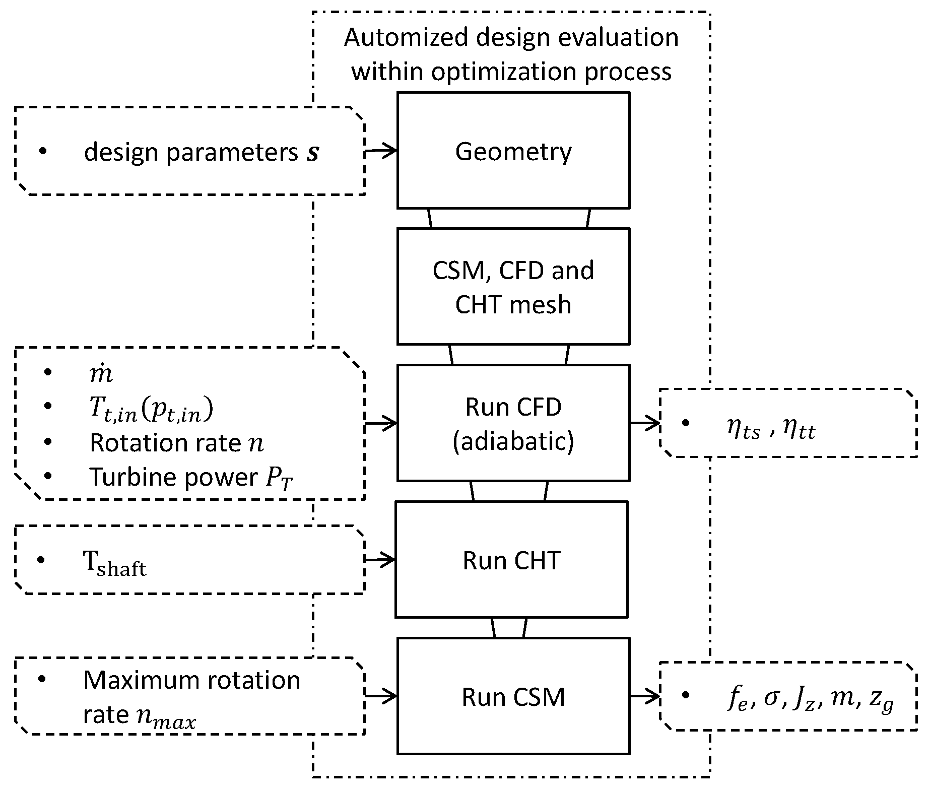
Figure 1 visualizes the gradient-free workflow, which will be explained in this first part of the paper. Initially, a fluid and a solid geometry are created and meshed based on a parametrized CAD model and a parameter set . The simulation is performed in three steps: First, an adiabatic CFD (Computational Fluid Dynamics) simulation is conducted to calculate the efficiency . Second, the solid mesh is activated to facilitate a CHT (Conjugate Heat Transfer) calculation that is initialized with the aforementioned CFD flow field. Finally, the CSM (Computational Structural Mechanics) is run, i.e., the temperature field in the solid, the surface pressure distribution and the rotation rate are used to calculate both the eigenfrequencies and the stresses. Furthermore, the rotor mass m, the center of gravity , and the inertia are calculated. The workflow is wrapped within an optimization software that implements a meta-model assisted genetic algorithm described and detailed at the end of this chapter.
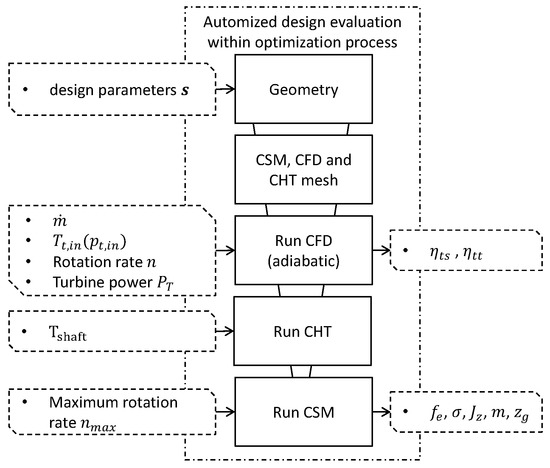
Figure 1.
Gradient-free setup.
2.1. Geometry Parametrization
The CAD geometry is built using the 3D modeling software CAESES®. The blade is modeled in three steps:
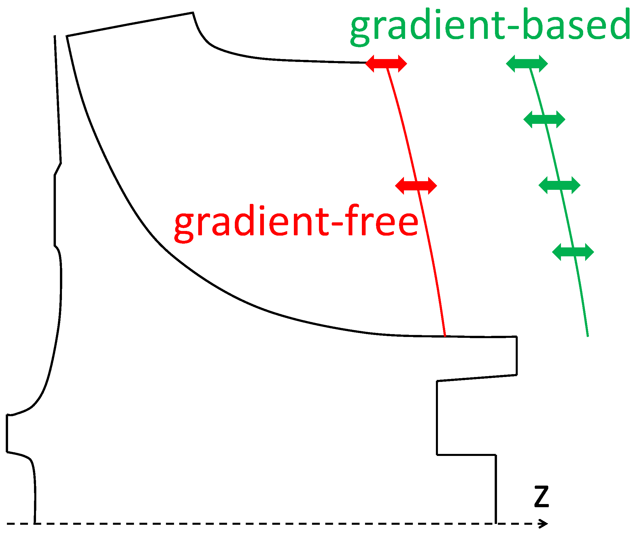
1. A meridional view of the blade is created using B-Splines, including the leading edge, trailing edge, hub, and shroud contour, see Figure 2. In the same step, the turbine back and outlet are designed.
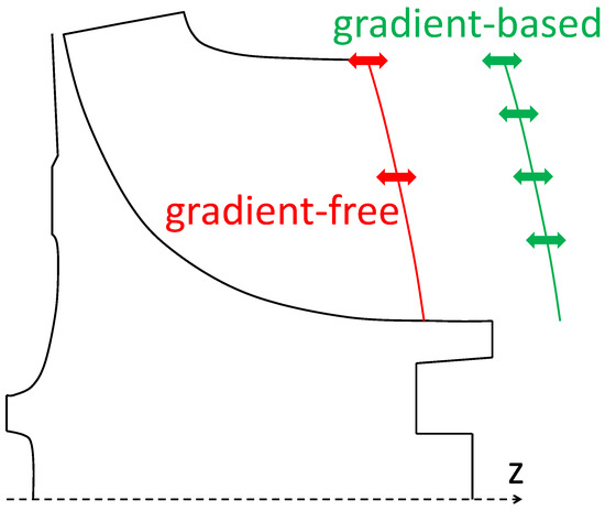
Figure 2.
Meridional view.
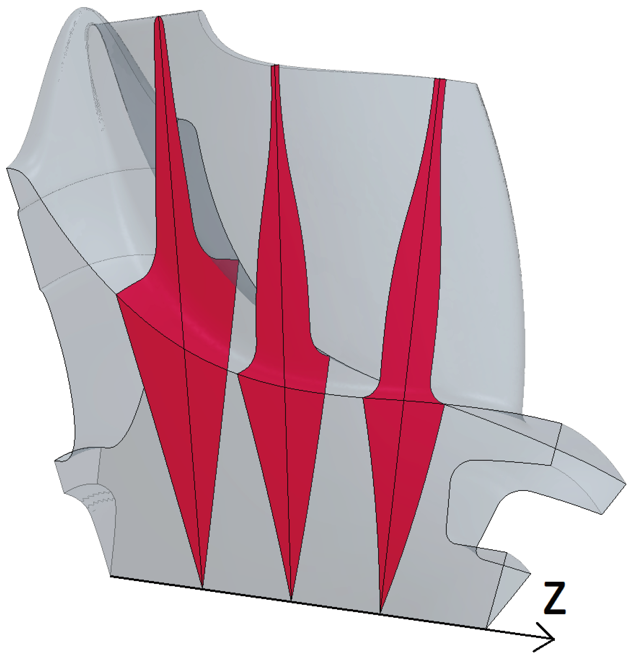
2. The blade camber surface is created based on the meridional surface by specifying a -distribution at hub, Figure 3, which is controlled via inlet angle and outlet angle plus two weighting points (red). The -distribution solely depends on the axial position z, and describes the peripheral angle. Consequently, the position of every point on the camber surface is fully defined by its radius r and its axial position z. The major benefit of this camber description is that it leads to radially fibered blades, Figure 4, that prevent bending stresses within the blades due to centrifugal forces.
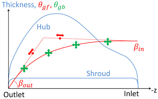
Figure 3.
Thickness and -distribution.

Figure 4.
Radially fibered blades.
3. Two splines are used to define a thickness distribution at both hub and shroud, Figure 3. A third spline is used to control the blending of the spanwise thickness.
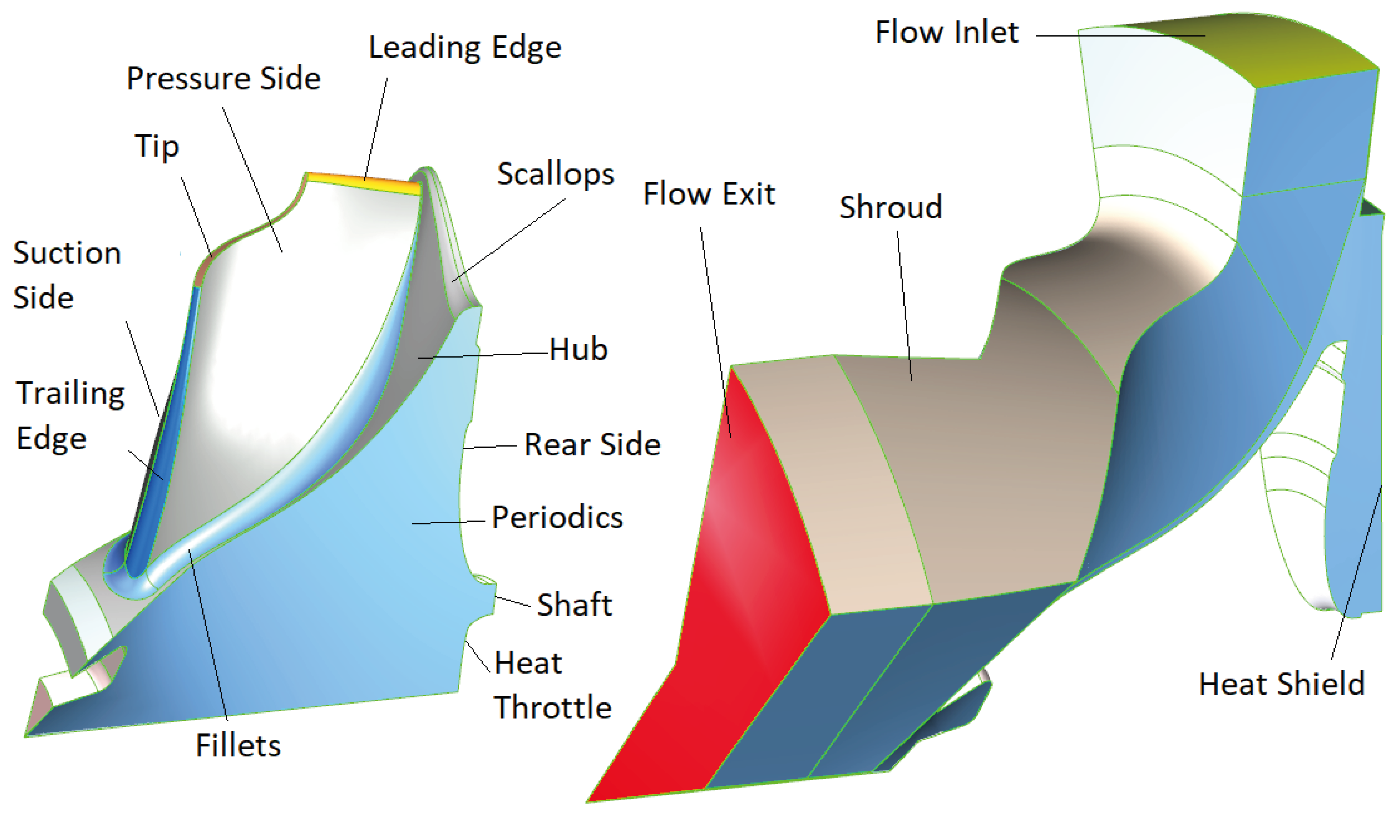
The model includes several further important features, Figure 5: Internally, the largest possible fillet radius is calculated based on the smallest distance of two adjacent blades. The latter mostly depends on the chosen number of blades and its hub thickness. This result is used to design the variable fillet connection of blade and hub geometry and is automatically chosen as large as possible to minimize the stresses in the fillets. The model also includes parameters to control the scallops. They are used to steer the inertia of the rotor and the stresses at the turbine rear side. The fluid geometry includes the gap between the heat shield and the rotor. The shroud tip gap can be defined, and both length and diameter of the diffuser can be set. However, these parameters are fixed during the optimization. In total, parameters, including the number of blades, are varied during optimization, see Table 1.
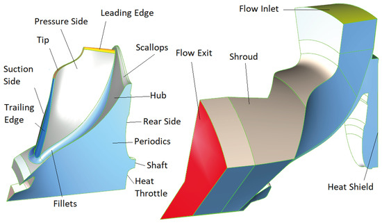
Figure 5.
Solid (l.) and fluid (r.) body.

Table 1.
Variable parameters for gradient-free and gradient-based setup
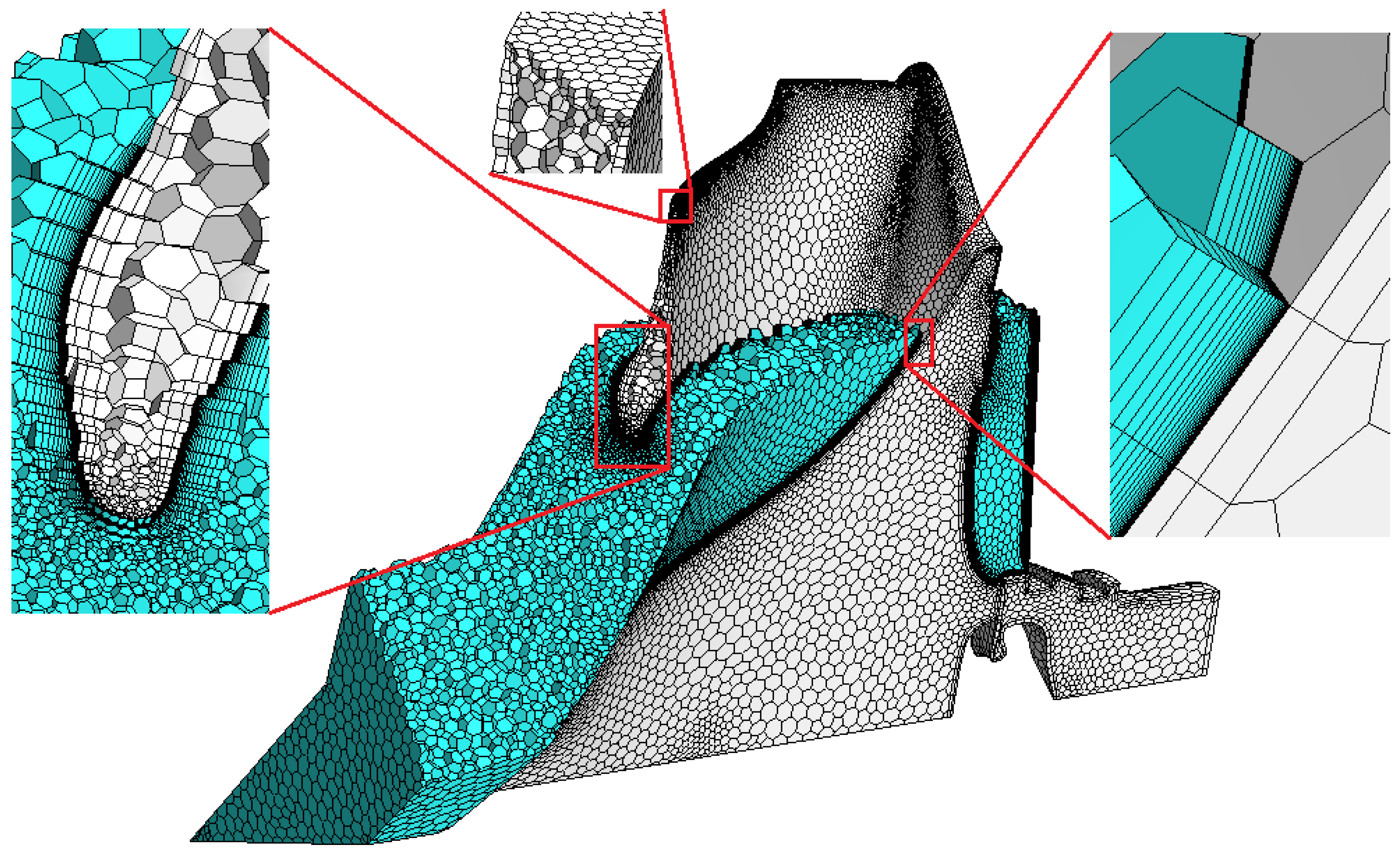
Eventually, the heat transfer calculations are substantially simplified as the fluid and the solid body share the same periodic surfaces, i.e., the fluid-solid-interface has a perfect overlap, see Figure 6.
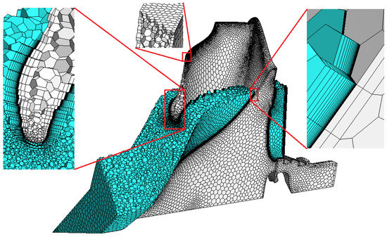
Figure 6.
Mesh for CFD and CHT.
2.2. Meshes
The solid geometry for CSM is meshed with Altair SimLab producing roughly 80.000 tetrahedral second-order elements. Table 2 presents a mesh study with three different meshes. A Richardson extrapolation [8] is used to calculate an estimate for the asymptotic values of the eigenfrequency and von Mises stresses . The relative extrapolated error
shows that a high uncertainty of must be expected. This observation is not surprising as small radii lead to high stress concentrations and therefore require many elements.

Table 2.
Mesh study on CSM mesh.
The fluid geometry for CFD and the solid geometry for CHT are meshed with unstructured polyhedrals using the Star-CCM+ meshing capabilities. Prism layers with a stretching of 1.2 are used to resolve the boundary layer, which maintains and leads to approximately 1 million cells in total. The flow outlet is elongated with a mesh extrusion. Table 3 summarizes a mesh study that once more uses a Richardson extrapolation to get an estimate for the asymptotic solution. The relative extrapolated error is considered reasonably small.

Table 3.
Mesh study on CFD mesh.
Even though block-structured meshes offer a higher ratio of accuracy to computational cost, unstructured meshes are preferred here, since they offer the flexibility to mesh the fillets, scallops, and heatshield gap. Furthermore, a node-conformal mesh at the interface between solid and fluid can be created, Figure 6. This facilitates a robust simulation of the turbine temperature field.
2.3. Simulation Setup
After the meshes have been generated, an adiabatic CFD calculation in Star-CCM+ is conducted. The boundary conditions are set as follows: The inlet mass flow and the back pressure are fixed. In absence of a volute, an inlet flow angle has to be set and is adjusted during simulation to assure that the turbine is delivering the target power . The angle is increased when the current power is too high and vice versa. This way, , which is connected to the turbine inlet temperature in piston engines, is not known a priori. A simple, linear way ([9], p. 30) is used to model this dependency to set the inlet temperature dynamically
where and are in-cylinder temperature and pressure at valve opening. The flow is assumed fully turbulent. The Reynolds number based on the inlet width b is , which is why a turbulent velocity profile is set at the inlet, i.e.,
with r as the distance from the mid of the inlet channel. The -model is used for closure of the RANS equations.
After convergence of the CFD simulation, the polyhedral mesh of the solid region is activated, Figure 7. A constant temperature is set at the shaft. Every other wall is assumed adiabatic, i.e., the shaft is the only heat sink and radiation is neglected. As this CHT simulation starts from a converged flow solution, it converges reasonably fast: . The temperature field is mapped onto the tetrahedral mesh as depicted in Figure 7. Additionally, the surface pressure distribution is mapped onto the surface of the tetrahedral mesh.
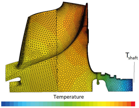
Figure 7.
Tetrahedrals (CSM, left), polyhedrals (CHT, right).
Subsequently, the von Mises stresses within the rotor are calculated with the open-source finite element code CalculiX [10] based on the maximum rotation rate , including both the previously calculated temperature and pressure field. While the temperature has a significant impact on the stresses, especially in the turbine back, the latter is almost negligible as it just slightly increases the stresses at the rotor-shaft-connection. The first blade eigenfrequency is calculated based on this pre-stressed state.
Lastly, inertia , mass m, and center of gravity are calculated. Gauss’s theorem is used, e.g.,
to calculate these quantities based on a tesselated STL file of the solid body surface.
The respective simulation runtimes are reported in Table 4.

Table 4.
Wall clock time within gradient-free setup.
2.4. Objectives and Constraints
Two objective values are maximized during the optimization: The total-to-static efficiency and the total-to-total efficiency, Equation (5):
These cost functions have a high correlation, yet, it is not one, see the final database in Figure 8. Maximizing is equivalent to assuming the exit kinetic energy after diffuser being a loss. However, within modern piston engines the radial turbine is not the last geometry in the exhaust piping system, i.e., there usually will be an exhaust after treatment (EAT). Consequently, from a system perspective, the stagnation pressure between turbine diffuser exit and EAT is important. Summarized, assuming having the choice between two designs with the same , then deciding for the one with the higher is reasonable.
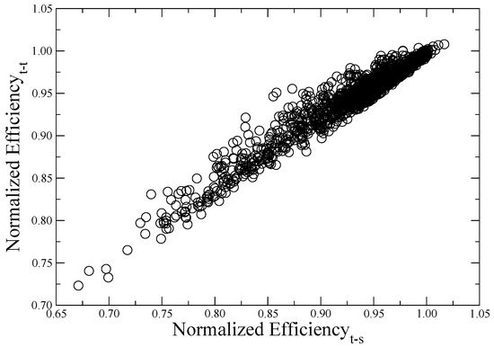
Figure 8.
Comparison of and .
Apart from these objectives, several constraints are considered:
The first eigenfrequency of the blade
is constrained to lie above a specific engine order (+ safety margin), which is an empirically chosen value. This constraint is set to prevent high cycle fatigue damages during operation.
The inertia of the turbine is constrained as it affects the turbocharger’s transient performance as a lower inertia leads to faster rotor acceleration. In that regard, the compressor inertia is not equally significant as its density is substantially lower due to different materials:
The rotor mass m is constrained as it slightly affects the manufacturing costs, but more importantly, influences the rotor dynamics as lower masses lead to smaller rotation orbits assuming comparable eccentricity and center of gravity. As such, it prevents the rotor from rubbing against the housing during operation even for small tip gaps. For the same reason, also the axial position of the center of gravity is constrained.
The von Mises stresses are constrained at two different surfaces where peaks are expected: On the fillet surface between two adjacent blades and at the turbine rear side, see Figure 5. The allowable stress is set well below the materials yield strength with a large safety margin as the turbine is designed to withstand a high number of load cycles. Furthermore, the stresses are evaluated in an integral sense as in [5], i.e.,
This formulation has a smoothing effect on the non-differentiable -evaluation. Consequently, it the quality of the applied meta-models and is less prone to mesh induced noise in the results. The optimization problem is summarized as follows:
2.5. Optimization Results
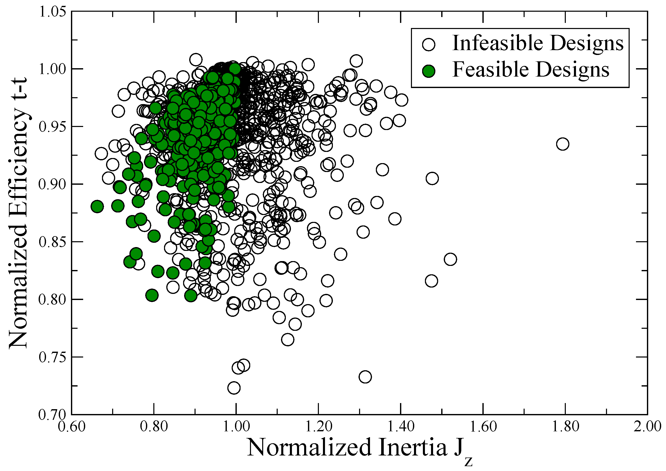
Based on the previously described workflow, the automated design evaluation is implemented within the optimization software modeFRONTIER. To sample the design space, first, a design of experiments is set up. A uniform Latin hypercube is used that delivers 395 successful design evaluations. Upon this database, the optimization is started exploiting one of the software’s implemented meta-model assisted multi-objective genetic algorithm (GA) called FAST MOGA II [11]. During the optimization, the software sets up four meta-models (polynomial SVDs, neural networks, radial basis functions, kriging) per output function and automatically chooses the most successful one for every function by comparing their prediction to the evaluated designs of the newest generation of designs. ’Success’ is determined by using a mean error. Afterwards, the new generation is added to the meta-model training base and the next generation is started. Another 1302 designs are assessed this way. 1697 designs are evaluated in total with 1105 being infeasible and violating at least one of the constraints, see Figure 9. The design with the highest efficiency fulfilling all constraints is picked and prepared for the subsequent design step, described in the next chapter. Figure 4, Figure 5, Figure 6 and Figure 7 show the chosen design. This design, coincidentally, is the one with the highest total-to-static efficiency , i.e., there is just one rank 1 Pareto design. Evaluating 1697 designs serially on 24 CPUs would have taken approximately 1300 h (see Table 4), so this process is very costly. This is driven by both the runtime per design and the 42 free parameters. Reducing the latter may drastically reduce the optimization runtime. However, deciding which parameters to render down is a difficult task on its own, which may either be guided by the designer’s experience or a prior sensitivity study. At last, this motivates the workflow presented in the next chapter as the number of free parameters has a marginal impact on the optimization runtime in the gradient-free setup.
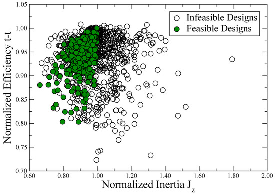
Figure 9.
Optimization results.
3. Gradient-Based Optimization
Figure 10 summarizes the process used to drive a gradient-based optimization of the radial turbine. The central idea is to locally approximate each response function linearly as
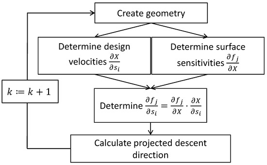
Figure 10.
Gradient-based optimization workflow.
A gradient projection algorithm is applied to drive an optimization aimed at raising the efficiency while satisfying several constraints. Calculating for every response function in a reasonable timeframe is, however, not straightforward:
Using finite differences is too costly as it would require design evaluations to approximate . Hence, the derivative is split via the chain rule
where X refers to the surface mesh node positions and is computed in a single simulation per response function. Still, evaluations are necessary to approximate ; however, these operations are cheap. Both steps are detailed below.
Unfortunately, not all response functions handled in the gradient-free framework are available in this gradient-based setting. In particular, the calculation of the stress sensitivity has not been included yet. One way to implement this has been presented by [12].
3.1. Altered Geometry Parametrization and Simulation Setup
To investigate whether the method is capable of further improving the design, the geometry is re-parametrized, i.e., two splines are exchanged to add further degrees of freedom. The two chosen splines describe the turbine trailing edge, and the -distribution, Figure 2 and Figure 3, sketched in red (old) and green (new). In total, it contains parameters (reminder: ). As the number of blades is a discontinuous parameter, it needs to be set constant.
The CFD simulation setup is adapted for this optimization: and remain fixed and a stagnation pressure at inlet is used, i.e., is set at the inlet. As might change as the design changes with these boundary conditions, it is now handled as a constraint.
The runtime of this setup changes compared to the gradient-free setup: The primal CFD run now takes approximately twice as long as going down to machine precision is advisable in the context of the subsequent adjoint calculation. The adjoint run takes approximately three times as long as the primal run accounting for two cost functions and the chosen GMRES solver. However, neither a temperature field nor stresses are calculated in this gradient-based setup.
3.2. Design Velocity
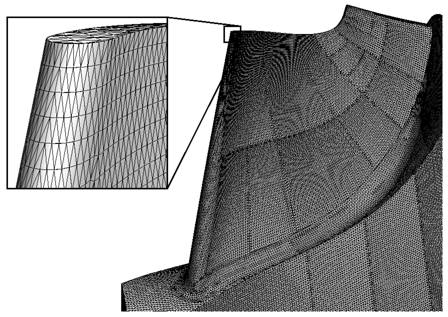
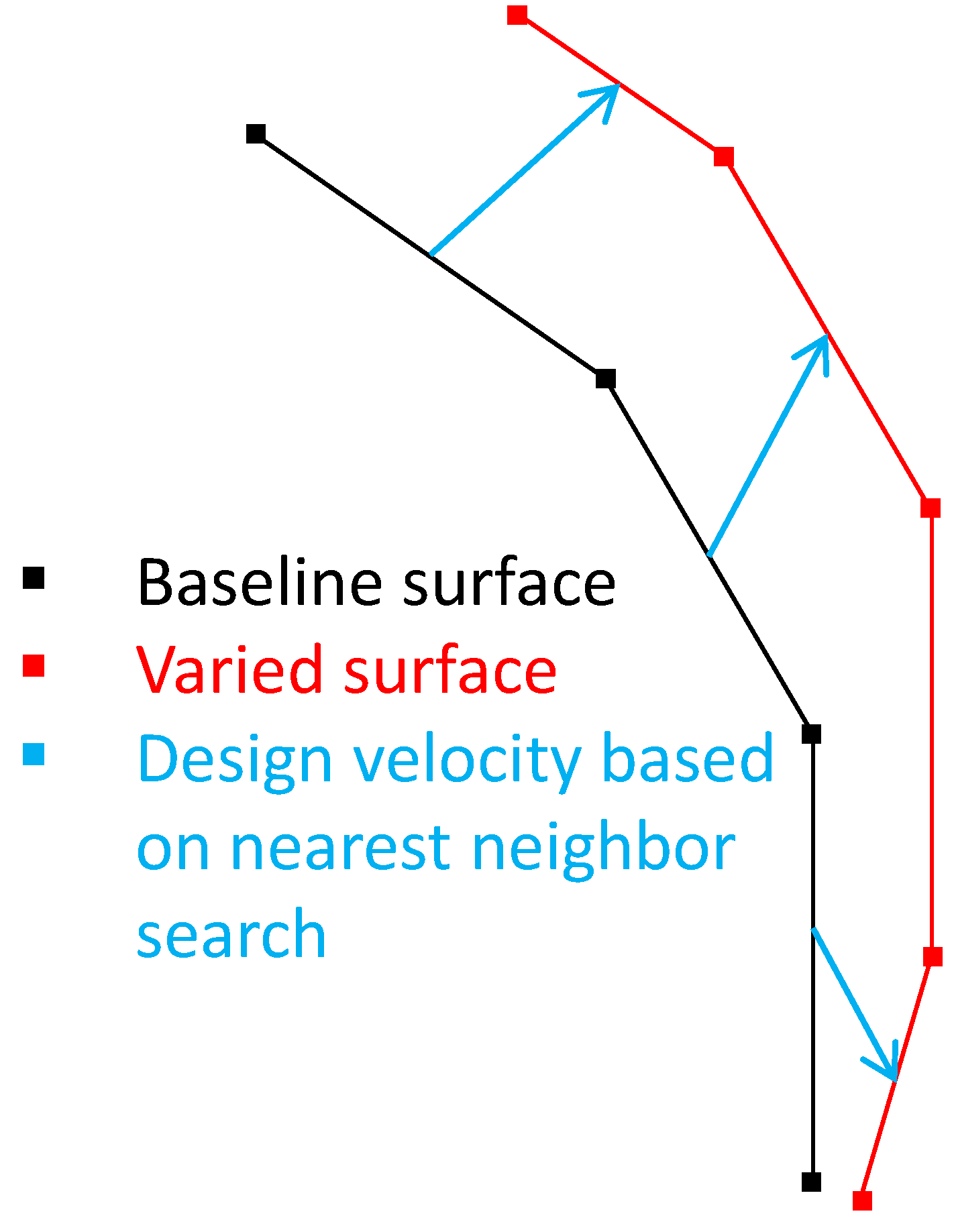
Tesselated surface descriptions, i.e., STL files, Figure 11, are used to calculate the design velocities with a first order finite differencing scheme, where X are the centers of the STL triangles and is a CAD parameter. To calculate the sensitivity, two geometries are necessary: The baseline geometry X based on the parameter set and , which is varied in one parameter by a small distance . The derivative is calculated pointwise
where , . Care must be taken as to which the point is compared to for the difference calculation in Equation (11). The nearest neighbor algorithm from Pythons SciPy library is used to find the point which is located closest to . The design velocity is calculated as in Equation (11) (depicted in blue in Figure 12).
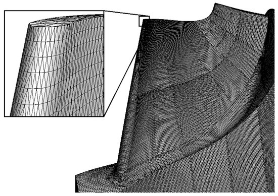
Figure 11.
Tesselated surface mesh.
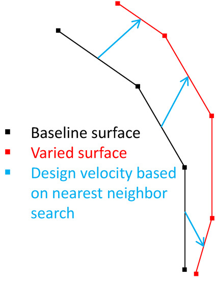
Figure 12.
Design velocity calculation.
3.3. Surface Sensitivity
The surface mesh sensitivity must be determined for every response function . The applied methods differ for the various responses:
The mesh sensitivities of both and are determined with the adjoint method, implemented in Star-CCM+, which allows for an efficient calculation of the gradients. Applying this method requires the solution of one additional system of equations per response, which are solved with a Krylov subspace scheme. The code implements the discrete adjoint approach, i.e., the derivation of the adjoint equations is based on the discretized Navier–Stokes Equations. The frozen turbulence assumption is used, i.e., the turbulent viscosity is assumed constant during the adjoint simulation. After calculation of the volume mesh sensitivities, only the sensitivities on the surface are used in the optimization. The values of the inner nodes are assumed negligible. Consequently, the sensitivity of the volume mesh regarding to the surface mesh neglected. For a general outline on this and related methods, see [13]. The total-to-static efficiency is no longer regarded: Gradient-based schemes in a multidisciplinary setting require compromise functions that weight individual objectives against each other, e.g., a weighted linear combination . In the following, however, we neglect s.t. .
The first eigenfrequency and its mesh sensitivity are calculated with the open-source code Kratos [14]. After the eigenvalue and its eigenvector have been determined, the calculation of the sensitivity with respect to a mesh node position can be found by differentiating the undamped eigenvalue equation to get
where M, K are the finite element mass and stiffness matrix, i.e., no further linear system must be solved. In Kratos, first order finite differences are used to determine both and . The mesh sensitivity of nodes not lying on the surface is neglected and assumed zero. For a derivation of Equation (12), see e.g., [15].
The surface sensitivity of , m, and can be determined analytically based on the tesselated surface. Take a triangle of the triangulated surface and let be its area. Assume this triangle being translated by in surface normal direction n. Then, the surface sensitivity of e.g., the inertia J is
In total, the optimization problem may be summarized as follows:
Please note that the subscript 1 refers to the values of design iteration 1, i.e., the chosen design at the end of the gradient-free optimization.
3.4. Gradient Calculation
Figure 13 exemplarily summarizes the steps described above. On the left, the surface sensitivity of the eigenfrequency is shown. In the middle, the design velocity of one parameter describing the blade thickness at shroud is presented. On the right, the pointwise product of these two is visualized, which is calculated using another nearest neighbor search. Integration along the surface finally delivers .

Figure 13.
Eigenfrequency sensitivity (left), design velocity (mid) and pointwise product (right).
3.5. Optimization Results
The gradient-based optimization is driven with a gradient projection algorithm, which facilitates the handling of both inequality and equality constraints, see [7], ch. 5: First, the gradient of the efficiency is orthogonally mapped into the subspace of all active, linearized constraints to calculate the projected descent direction. Equality constraints, such as the mass flow constraint, are always considered active, while inequality constraints including parameter boundaries are inactive as long as they are not violated. The second step is a damped correction step that copes with the difference between the target value and the actual value of the respective constraint. Finally, the chosen descent step is a linear combination of these two, i.e., projection and correction step.
The success of the optimization is tightly linked to the quality of the gradient approximation. Hence, a study based on forward differences is conducted to judge whether the presented chain of methods exploiting surface sensitivities and design velocities (SS+DV) delivers reasonable derivatives. However, determining a gradient via finite differences (FD) is expensive as the baseline design plus variations thereof must be evaluated to facilitate a finite difference gradient approximation. A comparison for a few cost functions is presented in Figure 14, where the dotted lines show the FD gradients, and the solid lines represent the derivatives based on the SS+DV approach for all parameters. The gradients , and match reasonably with only a few deviating parameters.

Figure 14.
, , each calculated both via finite differences (FD) and via surface sensitivities + design velocities (SS+DV).
The optimization runs successfully, see Figure 15. Within five iterations, the optimization stagnates. At this point, an increase in by 0.34% can be observed. Both the initial design and the design from iteration 8 are shown in Figure 16 for comparison. Figure 16 shows that the major design change lies in the -distribution. In iteration 4, the eigenfrequency drops below its constraint value, and the projected descent algorithm starts its correction steps. However, drifts away from its target value. This behavior indicates either imprecise gradients or a too strongly damped correction. The cost functions inertia , center of gravity , and rotor mass m hardly change throughout the optimization run, see Figure 15. Even though the stresses and have no longer been evaluated for the gradient-based setup, the minimal changes in geometry suggest that no major increase in stress has to be expected. Furthermore, it is worth mentioning that the total-to-static efficiency is hardly raised (∼0.1%). This result indicates that the change in is partly linked to an increased kinetic energy at the turbine outlet, i.e., the swirl is higher.
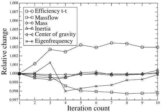
Figure 15.
Optimization run.
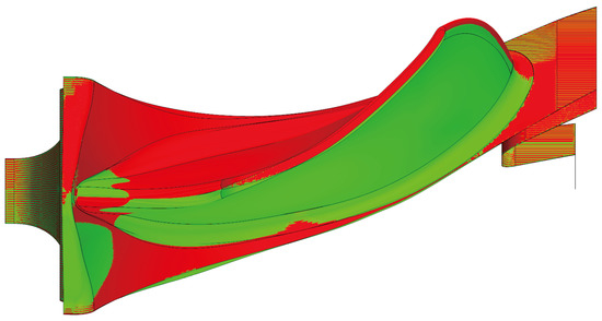
Figure 16.
Gradient-free design (iteration 1, red) and gradient-based design (iteration 8, green).
4. Conclusions
Two workflows to optimize a radial turbine with different advantages and disadvantages have been presented. They have shown to complement each other well: The gradient-free setup can be used to sample the design space and find a reasonable turbine design. Furthermore, it offers the possibility to handle discrete variables such as the number of blades. Yet, the designer is obliged to limit the number of free variables as computational cost becomes an issue, known as the curse of dimensionality. The gradient-based process allows for an increase in degrees of freedom without majorly affecting the computational costs. In fact, it is negligible compared to the costs that come along with the gradient-free setup. Within this study, the runtime of the gradient-based setup turned out to be two orders of magnitude lower: The runtime is driven by the primal and adjoint CFD simulations, which are more costly than in the gradient-free setup as mentioned earlier. Neglecting the CHT calculations, we estimate a ratio of
for this specific case. However, one must keep in mind that the gradient-free workflow started from scratch while the gradient-based workflow was initiated from an optimized design. Hence, no general conclusions on the runtimes of the workflows may be drawn.
Future work will focus on three aspects: First, the gradient-free setup will be supplemented with life-expectancy calculations that necessitate prior stress and temperature field simulations. Second, the gradient-based setup will be complimented with stress sensitivities to allow for a more holistic and comparable design chain. Third, the gradient quality of the flow-related sensitivities will be improved by dropping the frozen turbulence assumption and introducing a more sophisticated derivative of volume mesh regarding the surface mesh.
Author Contributions
Conceptualization, N.L.; funding acquisition, H.-P.S. and J.K.; investigation, N.L.; methodology, N.L. and D.B.; project administration, N.L.; supervision, H.-P.S. and J.K.; visualization, N.L.; writing, original draft, N.L.; writing, review and editing, N.L., D.B., H.-P.S. and J.K. All authors have read and agreed to the published version of the manuscript.
Funding
The authors acknowledge the financial support by the Federal Ministry for Economic Affairs and Energy of Germany (BMWi) in the project GAMMA (project number 03ET1469a). The APC of this paper was funded by Euroturbo.
Acknowledgments
We gratefully thank MTU Friedrichshafen GmbH for the permission to publish this paper and Friendship Systems for their support in building the CAD geometry.
Conflicts of Interest
The authors declare no conflicts of interest.
Abbreviations
The following abbreviations are used in this manuscript:
| Latin | |
| Extrapolated relative error | |
| Eigenfrequency | |
| Cost function j | |
| h | Specific enthalpy |
| J | Inertia |
| K | Stiffness matrix |
| Mass flow | |
| m | Rotor mass |
| M | Mass matrix |
| n | Rotation rate |
| p | Pressure |
| Parameter set | |
| T | Temperature |
| v | Velocity |
| Center of gravity | |
| Greek | |
| Isentropic exponent | |
| Efficiency | |
| Stress tensor | |
| Subscripts | |
| gradient-based | |
| gradient-free | |
| s | Static quantity |
| t | Stagnation quantity |
| Abbreviations | |
| CFD | Computational Fluid Dynamics |
| CHT | Conjugate Heat Transfer |
| CSM | Computational Structural Mechanics |
| GA | Genetic algorithm |
| RANS | Reynolds-averaged Navier–Stokes |
| STL | Standard Tesselation Language |
References
- Verstraete, T. Multidisciplinary Turbomachinery Component Optimization Considering Performance, Stress, and Internal Heat Transfer. Ph.D. Thesis, von Karman Institute for Fluid Dynamics—University of Gent, Gent, Belgium, 2008. [Google Scholar]
- Müller, L.; Alsalihi, Z.; Verstraete, T. Multidisciplinary Optimization of a Turbocharger Radial Turbine. J. Turbomach. 2013, 135. [Google Scholar] [CrossRef]
- Peter, J. Numerische Untersuchung und Optimierung des Laufrades einer Pkw-Abgasturboladerturbine. Ph.D. Thesis, Leibniz Universität Hannover, Hannover, Germany, 2016. [Google Scholar]
- Khairuddin, U.B.; Costall, A.W. Aerodynamic Optimization of the High Pressure Turbine and Interstage Duct in a Two-Stage Air System for a Heavy-Duty Diesel Engine. J. Eng. Gas Turbines Power 2018, 140. [Google Scholar] [CrossRef]
- Verstraete, T.; Müller, L.; Müller, J.D. Multidisciplinary Adjoint Optimization of Turbomachinery Components Including Aerodynamic and Stress Performance. In Proceedings of the 35th AIAA Applied Aerodynamics Conference, Denver, CO, USA, 5–9 June 2017. [Google Scholar]
- Schwalbach, M.; Verstraete, T.; Müller, L.; Gauger, N. CAD-Based adjoint multidisciplinary optimization of a radial turbine under structural constraints. In Proceedings of the Montreal 2018 Global Power and Propulsion Forum, Zug, Switzerland, 7–9 May 2018. [Google Scholar]
- Haftka, R.T.; Gürdal, Z.; Kamat, M. Elements of Structural Optimization (Solid Mechanics and Its Applications); Springer: Berlin/Heidelberg, Germany, 2013. [Google Scholar]
- Celik, I.B.; Ghia, U.; Roache, P.J.; Freitas, C.J.; Coleman, H.; Raad, P.E. Procedure for Estimation and Reporting of Uncertainty Due to Discretization in CFD Applications. J. Fluids Eng. 2008, 130. [Google Scholar] [CrossRef]
- Pucher, H.; Zinner, K. Aufladung von Verbrennungsmotoren: Grundlagen, Berechnungen, Ausführungen (German Edition); Springer: Berlin/Heidelberg, Germany, 2012. [Google Scholar]
- Dhondt, G.; Wittig, K. Calculix: A Free Software Three-Dimensional Structural Finite Element Program; MTU AeroEngines: Munich, Germany, 1998. [Google Scholar]
- Montrone, T.; Turco, A.; Rigoni, E. FAST Optimizers: General Description; Esteco Technical report; Esteco: Trieste, Italy, 2014. [Google Scholar]
- Verstraete, T.; Müller, L.; Müller, J.D. CAD-Based Adjoint Optimization of the Stresses in a Radial Turbine. In Proceedings of the ASME Turbo Expo 2017, Charlotte, NC, USA, 26–30 June 2017. [Google Scholar]
- Peter, J.E.; Dwight, R.P. Numerical sensitivity analysis for aerodynamic optimization: A survey of approaches. Comput. Fluids 2010, 39, 373–391. [Google Scholar] [CrossRef]
- KRATOS-Multiphysics. Available online: https://github.com/KratosMultiphysics/Kratos (accessed on 30 September 2018).
- Firl, M. Optimal Shape Design of Shell Structures. Ph.D. Thesis, Chair of Structural Mechanics—Technical University of Munich, Munich, Germany, 2010. [Google Scholar]
© 2020 by the authors. Licensee MDPI, Basel, Switzerland. This article is an open access article distributed under the terms and conditions of the Creative Commons Attribution (CC BY) license (http://creativecommons.org/licenses/by/4.0/).

