Abstract
The paper presents a state-of-the-art review of turbine trailing edge flows, both from an experimental and numerical point of view. With the help of old and recent high-resolution time resolved data, the main advances in the understanding of the essential features of the unsteady wake flow are collected and homogenized. Attention is paid to the energy separation phenomenon occurring in turbine wakes, as well as to the effects of the aerodynamic parameters chiefly influencing the features of the vortex shedding. Achievements in terms of unsteady numerical simulations of turbine wake flow characterized by vigorous vortex shedding are also reviewed. Whenever possible the outcome of a detailed code-to-code and code-to-experiments validation process is presented and discussed, on account of the adopted numerical method and turbulence closure.
1. Introduction
The first time the lead author came in touch with the problematic of turbine trailing edge flows was in 1965 when, as part of his diploma thesis, which consisted mainly in the measurement of the boundary layer development around a very large scale HP steam turbine nozzle blade, he measured with a very thin pitot probe a static pressure at the trailing edge significantly below the downstream static pressure. This negative pressure difference explained the discrepancy between the losses obtained from downstream wake traverses and the sum of the losses based on the momentum thickness of the blade boundary layers and the losses induced by the sudden expansion at the trailing edge. Pursuing his curriculum at the von Kármán Institute the author was soon in charge of building a small transonic turbine cascade tunnel with a test section of 150 × 50 mm, the C2 facility, which was intensively used for cascade testing for industry and in-house designed transonic bladings for gas and steam turbine application. These tests allowed systematic measurements of the base pressure as part of the blade pressure distribution for a large number of cascades which were first presented at the occasion of a Lecture Series held at the von Kàrmàn Institute (VKI) in 1976 and led to the publication of the well-known VKI base pressure correlation published in 1980. This correlation has served ever since for comparison with new base pressure data obtained in other research labs. Among these let us already mention in particular the investigations carried out on several turbine blades at the University of Cambridge, published in 1988, at the University of Carlton, published between 2001 and 2004, and at the Moscow Power Institute, published between 2014 and 2018.
In parallel to these steady state measurements, the arrival of short duration flow visualizations and the development of fast measurement techniques in the 1970’s allowed to put into evidence the existence of the von Kármán vortex streets in the wakes of turbine blades. Pioneering work was performed at the DLR Göttingen in the mid-1970’s, with systematic flow visualizations revealing the existence of von Kármán vortices on a large number of turbine cascades in the mid-seventies. This was the beginning of an intense research on the effect of vortex shedding on the trailing edge base pressure. A major breakthrough was achieved in the frame of two European research projects. The first one, initiated in 1992, Experimental and Numerical Investigation of Time Varying Wakes Behind Turbine Blades (BRITE/EURAM CT92-0048, 1992–1996) included very large-scale cascade tests in a new VKI cascade facility with a much larger test section allowing the testing of a 280 mm chord blade in a three bladed cascade at a moderate subsonic Mach number, with emphasis on flow visualizations and detailed unsteady trailing edge pressure measurements. The VKI tests were completed by low speed tests at the University of Genoa on the same large-scale profile for unsteady wake measurements using LDV. In the follow-up project Turbulence Modelling of Unsteady Flows on Flat Plate and Turbine Cascades in 1996 (BRITE/EURAM CT96-0143, 1996-1999) VKI extended the blade pressure measurements on a 50% reduced four bladed cascade model to a high subsonic Mach number, Both programs not only contributed to an improved understanding of unsteady trailing edge wake flow characteristics, of their effect on the rear blade surface and on the trailing edge pressure distribution, but also offered unique test cases for the validation of unsteady Navier-Stokes flow solvers.
A special and unexpected result of the research on unsteady turbine blade wakes was the discovery of energy separation in the wake leading to non-negligible total temperature variations within the wake. This effect was known from steady state tests on cylindrical bodies since the early 1940’s, but its first discovery in a turbine cascade was made at the NRAC, National Research Aeronautical Laboratory of Canada, in the mid-1990s within the framework of tests on the performance of a nozzle vane cascade at transonic outlet Mach numbers. The experimental results of the total temperature distribution in the wake of cascade at supersonic outlet Mach number served many researchers, in particular from the University of Leicester, for elaborating on the effect of energy separation.
The paper starts with the evaluation of the VKI base pressure correlation (Section 2) in view of new experiments. This is followed with a review of the advances in the understanding of unsteady trailing edge wake flows (Section 3), the observation and explanation of energy separation in turbine blade wakes (Section 4), the effect of vortex shedding on the blade pressure distribution (Section 5) and the effect of Mach number and boundary layer state on the vortex shedding frequency (Section 6). This experimental part is complemented with a review of the numerical methods and modelling concepts as applied to the simulation of unsteady turbine wake characteristics using advanced Navier-Stokes solvers. Available numerical data documenting significant vortex shedding affecting the turbine performance even in a time averaged sense, are collected and compared on a code-to-code and code-to-experiments basis in Section 7.
2. Turbine Trailing Edge Base Pressure
Traupel [1], was probably the first to present in his book Thermische Turbomaschinen, a detailed analysis of the profile loss mechanism for turbine blades at subsonic flows conditions. The total losses comprised three terms: the boundary losses including the downstream mixing losses for infinitely thin trailing edges, the loss due to the sudden expansion at the trailing edge (Carnot shock) for a blade with finite trailing edge thickness taking into account the trailing edge blockage effect and a third term which did take into account that the static pressure at the trailing edge differed from the average static pressure between the pressure side (PS) and the suction side (SS) trailing edges across one pitch. Thus, the profile loss coefficient reads:
where:
is the dimensionless average momentum thickness, and:
the dimensionless thickness of the trailing edge. The constant appearing at the right-hand-side of Equation (1) depends on the ratio:
that is, for and for , while a linear variation of is used for . Terms containing squares and products of were considered to be negligible.
Most researchers are, however, more familiar with a similar analysis of the loss mechanism by Denton [2], who introduced in the loss coefficient expression , the term quantifying the trailing edge base pressure contribution, with:
For commodity may be taken as the isentropic downstream velocity . However, there was a big uncertainty as regards the magnitude of this term, although it appeared that it could become very important in the transonic range and explain the presence of a strong local loss maximum as demonstrated in Figure 1, which presents a few examples of early transonic cascades measurements performed at VKI and the DLR.
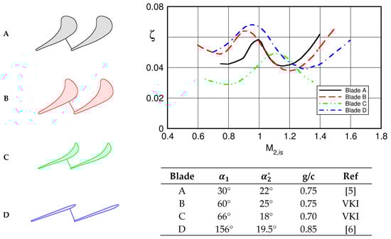
Figure 1.
Blade profile losses versus isentropic outlet Mach number for four transonic turbines. Blade A data from [5], blade B and C unpublished data from VKI, blade D data from [6].
Pioneering experimental research concerning the evolution of the turbine trailing edge base pressure from subsonic to supersonic outlet flow conditions was carried out at the von Kármán Institute. In 1976, at the occasion of the VKI Lecture Series Transonic Flows in Axial Turbines, Sieverding presented base pressure data for eight different cascades for gas and steam turbine blade profiles over a wide range of Mach numbers [3] and in 1980 Sieverding et al. [4] published a base pressure correlation (also referred to as BPC) based on a total of 16 blade profiles.
All tests were performed with cascades containing typically 8 blades and care was taken to ensure in all cases, and over the whole Mach range, a good periodicity. The latter was quantified to be 3%, in the supersonic range, in terms of the maximum difference between the pitch-wise averaged Mach number (based on 10 wall pressure tappings per pitch) of each of the three central passages and the mean value computed over the same three passages. The correlation covered blades with a wide range of cascade parameters, as outlined in Table 1:

Table 1.
Parameters range for Sieverding’s correlation.
Of all cascade parameters only the rear suction side turning angle and the trailing edge wedge angle appeared to correlate convincingly the available data, although the latter were insufficient to differentiate their respective influence. In fact, in many blade designs both parameters are closely linked to each other and, for two thirds of all convergent blades with convex rear suction side, both and were of the same order of magnitude. For this reason, it was decided to use the mean value as parameter. The relation , is graphically presented in Figure 2. The curves cover a range from to , but flow conditions characterized by a suction side shock interference with the trailing edge wake region are not considered. Comparing the experiments with the correlation (results not shown herein), it turned out that 80% of all data fall within a bandwidth and 96% within .
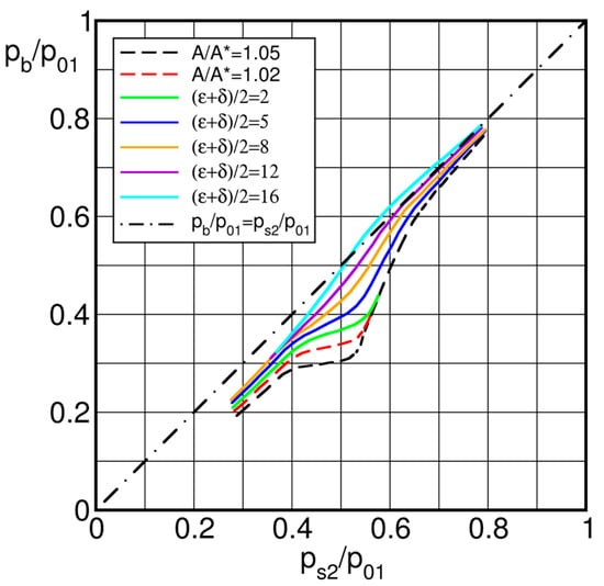
Figure 2.
Sieverding’s base pressure correlation; solid lines (resp. dashed lines) denote convergent blades (resp. convergent-divergent blades) [4].
An explanation for the significance of for the trailing edge base pressure is seen in Figure 3, presenting the blade velocity distribution for two convergent blades with different rear suction side turning angles of = 20° and 4.5°, blade A and B, together with a convergent/divergent blade with an internal passage area increase of , blade C. The curves end at because beyond, the pressure distribution is influenced by the acceleration around the trailing edge.
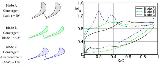
Figure 3.
Surface isentropic Mach number distribution for two convergent and one convergent/divergent blades at , based on data from [3].
The rear suction side turning angle ε has a remarkable effect on the pressure difference across the blade near the trailing edge. For blade A one observes a strong difference between the SS and PS isentropic Mach numbers, respectively pressures, while the difference is very small for blade B. On the contrary, for blade C the pressure side curve crosses the SS curve well ahead of the trailing edge and the PS isentropic Mach number near the trailing edge exceeds considerably that of the SS. The base pressure is function of the blade pressure difference upstream of the trailing edge.
It is also worthwhile mentioning that also plays an important role for the optimum blade design in function of the outlet Mach number. Figure 4 presents design recommendations for the rear suction side curvature with increasing Mach number from subsonic to low supersonic Mach numbers as successfully used at VKI.
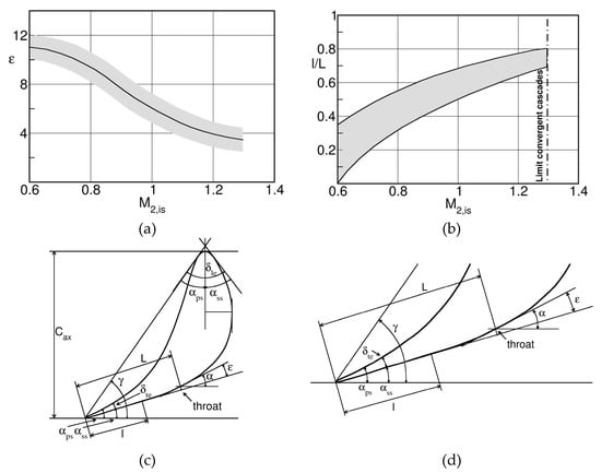
Figure 4.
Recommended values of (a) and (b) for the design of the blade rear suction side for increasing outlet Mach numbers. Full (c) and close-up (d) view of the parameters characterizing the turbine geometry.
The rear suction turning angle for convergent blades should decrease with increasing Mach number reaching a minimum of at (maximum Mach number for convergent blades). Note that similar trends can be derived from the loss correlation by Craig and Cox [7]. They showed that in order to minimize the blade profile losses the rear suction side curvature, expressed by the ratio , where represents the pitch and the radius of a circular arc approximating the rear suction side curvature, should decrease with increasing Mach number.
For a given rear suction side angle ε the designer is free as regards the evolution of the surface angle from the throat to the trailing edge. It appears to be a good design practice to subdivide the rear suction side length into two parts, a first part along which the blade angle asymptotically decreases to the value of the trailing edge angle, followed by a second entirely straight part of length , see Figure 4. With increasing outlet Mach number, the length of the straight part, that is the ratio increases, but it does never extend up to the throat.
For calculating the trailing edge losses induced by the difference between the base pressure and the downstream pressure, Fabry & Sieverding [8], presented the data for the convergent blades in Figure 2 in terms of the base pressure coefficient , defined by Equation (2), see Figure 5.
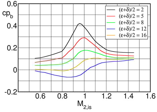
Figure 5.
Base pressure coefficients corresponding to the base pressure curves of Figure 2 [8].
Since the base pressure losses are proportional to the base pressure coefficient , the curves give immediately an idea of the strong variation of the profile losses in the transonic range. As regards the low Mach number range, the contribution of the base pressure loss is implicitly taken into account by all loss correlations. Therefore the base pressure loss is not to be added straight away to the profile losses as predicted for example with the methods by Traupel [1] and Craig and Cox [7] but rather as a difference with respect to the profile losses at :
Martelli and Boretti [9], used the VKI base pressure correlation for verifying a simple procedure to compute losses in transonic turbine cascades. The surface static pressure distribution for a given downstream Mach number is obtained from an inviscid time marching flow calculation.
An integral boundary layer calculation is used to calculate the momentum thickness at the trailing edge before separation. The trailing edge shocks are calculated using the base pressure correlation. Two examples are shown in Figure 6. Calculation of eight blades showed that 80% of the predicted losses were within the range of the experimental uncertainty.
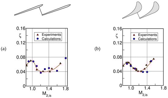
Figure 6.
Example of profile loss prediction for transonic turbine cascade, adapted from [9]; (a) low pressure steam turbine tip section, (b) high pressure gas turbine guide vane.
Besides the data reported by Sieverding et al. in [4,6], the only authors who published recently a systematic investigation of the effect of the rear suction side curvature on the base pressure were Granovskij et al. of the Moscow Power Institute [10]. The authors investigated 4 moderately loaded rotor blades (, , , ) with different unguided turning angles ( to 16°) in the frame of the optimization of cooled gas turbine blades. A direct comparison with the VKI base pressure correlation is difficult because the authors omitted to indicate the trailing edge wedge angle . Nevertheless, a comparison appeared to be useful. Figure 7 presents the comparison, after conversion, of the base pressure coefficient:
used by Granovskij et al. [10], to the base pressure coefficient (2) based on , used by Fabry and Sieverding at VKI [8]. The data of Granovskij et al. [10] (dashed lines) confirm globally the overall trends of the VKI base pressure correlation (solid lines). However, the peaks in the transonic range are much more pronounced.
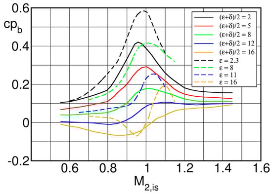
Figure 7.
Comparison of Granovskij’s base pressure data (dashed lines) with the VKI base pressure correlation (solid lines).
Also, cascade data reported by Dvorak et al. in 1978 [11] on a low pressure steam turbine rotor tip section, and by Jouini et al. in 2001 [12] for a relatively high turning rotor blade (, and a smaller pitch to chord ratio ), are in fair agreement with the VKI base pressure correlation, although the latter authors state that below , their data drop below those of the BPC.
However, some other cascade measurements deviate very significantly from the VKI curves. Deckers and Denton [13], for a low turning blade model and Gostelow et al. [14] for a high turning nozzle guide vane, report base pressure data far below those of Sieverding’s BPC, while Xu and Denton [15], for a very highly loaded HP gas turbine rotor blade ( and ) report base pressure data far above those of the BPC.
The simplicity of Sieverding’s base pressure correlation was often criticized because it was felt that aspects as important as the state of the boundary layer, the ratio of boundary layer momentum to trailing edge thickness and the trailing edge blockage effects (trailing edge thickness to throat opening) should play an important role.
As regards the state of the boundary layer and its thickness, tests on a flat plate model at moderate subsonic Mach numbers in a strongly convergent channel by Sieverding and Heinemann [16], showed that the difference of the base pressure for laminar and turbulent flow conditions was only of the order of 1.5–2% of the dynamic head of the flow before separation from the trailing edge. For the case of supersonic trailing edge flows, Carriere [17], demonstrated, that for turbulent boundary layers the base pressure would increase with increasing momentum thickness. On the contrary, supersonic flat plate model tests simulating the overhang section of convergent turbine cascades with straight rear suction sides showed that for fully expanded flow along the suction side (limit loading condition) an increase of the ratio of the boundary layer momentum to the trailing edge thickness by a factor of two, obtained roughening the blade surface, did not affect the base pressure, Sieverding et al. [18]. Note, that for both the smooth and rough surface the boundary layer was turbulent. Similarly, roughening the blade surface in case of shock boundary layer interactions on the blade suction side did not affect the base pressure as compared to the smooth blade, Sieverding and Heinemann [16]. However, a comparison of the base pressure for the same Mach numbers before separation at the trailing edge for a fully expanding flow and a flow with shock boundary layer interaction on the suction side before the TE showed an increase of the base pressure by 10–25 % in case of shock interaction before the TE. Since it was shown before that an increase of the momentum thickness did not affect the base pressure, the difference may be attributed to (a) different total pressures due to shock losses for the shock interference curve, (b) differences in the boundary layer shape factor and (c) differences in pressure gradients in stream-wise direction in the near wake region.
A systematic investigation of possible effects of changes in shape factor and boundary layer momentum thickness on the base pressure in cascades is difficult. Hence, the investigations are mostly confined to variations of the incidence angle which, via a modification of the blade velocity distribution, should have an impact on both the shape factor and the boundary layer momentum thickness. Based on linear transonic cascade tests on two high turning rotor blades Jouini et al. [19] at Carlton University, (blade HS1A: = 0.73, 0.082, , , , ; blade HS1B is similar to HS1A, but with less loading on the front side and ) concluded that discrepancies in the base region did not appear to be strongly related to changes of the inlet angle by , however in broad terms the weakest base pressure drop in the transonic range were obtained for high positive incidence. Similarly, experiments at VKI on a high turning rotor blade ( = 0.49, 0.082, , , , ) did not show any effect on the base pressure for incidence angle changes of [3].
In conclusion it appears that for conventional blade designs, changes in the boundary layer thickness alone, as induced by incidence variations, do not affect significantly the base pressure. Therefore, we need to look for possible other influence factors.
Figure 3 showed that the effect of the blade rear suction side blade turning angle ε on the base pressure was in fact function of the pressure difference across the blade near the trailing edge. Inversely, one should be able to deduct from the rear blade loading the tendency of the base pressure. The higher the blade loading at the trailing edge, the higher the base pressure. Corollary, a low or even negative blade loading near the trailing edge causes increasingly lower base pressures. This might help in explaining the large differences with respect to the BPC as found by Xu and Denton [15] on one side and Deckers et al. [13] and Gostelow et al. [14], mentioned before, on the other side.
To illustrate this, Figure 8 presents the base pressure data of Xu and Denton [15] for three of a family of four very highly loaded gas turbine rotor blades with a blade turning angle of and a pitch-to-chord , tested with three different trailing edge thicknesses. The blades are referred to as blade RD, for the datum blade, and blades DN and DK for changes of 0.5 and 1.5 times the trailing edge thickness with respect to the datum case.
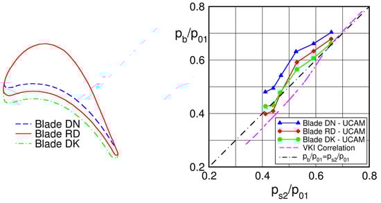
Figure 8.
Base pressure variation for blades of Xu & Denton; blade RD datum case, blade DK thick trailing edge, blade DN thin trailing edge. Adapted from [15].
The base pressures are overall much higher than those of the BPC which are indicated in the figure by the dashed line for a mean value of .
A possible explanation for the large differences is given by comparing the blade Mach number distribution of the datum blade with that of a VKI blade with a taken from [6], see Figure 9. To enable the comparison, the blade Mach number distribution of Xu & Denton (solid line) presented originally in function of the axial chord , had to be replotted in function of . The comparison is done for an isentropic outlet Mach number .
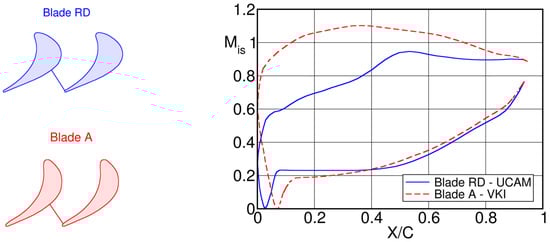
Figure 9.
Comparison of blade Mach number distribution for blade RD of Xu and Denton [15], (solid curve, ) with VKI blade (dashed curve, ).
Note that the geometric throat for the Xu & Denton blade is situated at , while for the VKI blade at . At the trailing edge, the Mach number difference between pressure and suction side for both blades are exactly the same, but contrary to the nearly constant Mach number for the VKI blade downstream of the throat, the blade of Xu and Denton is characterized by a very strong adverse pressure gradient in this region. As pointed out by the authors, this causes the suction side boundary layer to be either separated or close to separation up-stream of the trailing edge. Clearly, Sieverding’s correlation cannot deal with blade designs characterized by very strong adverse pressure gradients on the rear suction side causing boundary layer separation before the trailing edge.
The possible effect of boundary layer separation resulting from high rear suction side diffusion resulting in high base pressures was also mentioned by Corriveau and Sjolander in 2004 [20], comparing their nominal mid-loaded rotor blade HS1A, mentioned already before, with an aft- loaded blade HS1C with an increase of the suction side unguided turning angle from 11.5° to 14.5°. It appears that the increased turning angle could cause, in the transonic range, shock induced boundary layer transition near the trailing edge with, as consequence, a sharp increase of the base pressure, i.e., a sudden drop in the base pressure coefficient as seen in Figure 10. Note that the reported in the figure has been converted to of the original data.
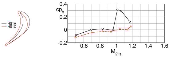
Figure 10.
Base pressure coefficient for mid-loaded (solid line) and aft-loaded (dashed line) rotor blade. Symbols:  HS1A geometry,
  HS1C geometry. Adapted from [20].
HS1A geometry, HS1C geometry. Adapted from [20].
As regards the base pressure data by Deckers and Denton [13] for a low turning blade model and Gostelow et al. [14] for a high turning nozzle guide vane, who report base pressure data far below those of Sieverding’s BPC, their blade pressure distribution resembles that of the convergent/divergent blade C in Figure 3 with a negative blade loading near the trailing edge which would explain the very low base pressures. In addition, the blade of Deckers and Denton has a blunt trailing edge, and there is experimental evidence that, compared to a circular trailing edge, the base pressure for blades with blunt trailing edge might be considerably lower. Sieverding and Heinemann [16] report for flat plate tests at moderate subsonic Mach numbers a drop of the base pressure coefficient by 11% for a plate with squared trailing edge compared to that with a circular trailing edge.
It is important to remember that the measurement of the base pressure carried out with a single pressure tapping in the trailing edge base region implies the assumption of an isobaric trailing edge pressure distribution. However, in 2003 Sieverding et al. [21] demonstrated that at high subsonic Mach numbers the pressure distribution could be highly non-uniform with a marked pressure minimum at the center of the trailing edge base, as will be shown later in Section 5. Under these conditions it is likely that the base pressure measured with a single pressure hole does not reflect the true mean pressure. In addition, the measured pressure would depend on the ratio of the pressure hole to trailing edge diameter , which is typically in the range . This fact was also recognized by Jouini et al. [12], who mentioned the difficulties for obtaining representative trailing edge base pressures measurements: “It should also be noted that at high Mach numbers the base pressure varies considerably with location on the trailing edge and the single tap gives a somewhat limited picture of the base pressure behavior”. It is probably correct to say that differences between experimental base pressure data and the base pressure correlation may at least partially be attributed to the use of different pressure hole to trailing edge diameters by the various researchers.
Finally, it is important to mention that the trailing edge pressure is sensitive to the trailing edge shape as demonstrated by El Gendi et al. [22] who showed with the help of high fidelity simulation that the base pressure for blades with elliptic trailing edges was higher than for blades with circular trailing edges. Melzer and Pullan [23] proved experimentally that designing blades with elliptical trailing edges improved the blade performance. The reason is that an elliptic trailing edge reduces not only the wake width but causes also an increase of the base pressure compared to that of blades with a circular trailing edge. This suggests that inaccuracies in the machining of blades with thin trailing edges could easily lead to deviations from the designed circular trailing edge shape and thus contribute to the differences in the base pressure.
3. Unsteady Trailing Edge Wake Flow
The mixing process of the wake behind turbine blades has been viewed for a long time as a steady state process although it was well known that the separation of the boundary layers at the trailing edge is a highly unsteady phenomenon which leads to the formation of large coherent structures, known as the von Kármán vortex street. The unsteady character of turbine blade wakes is best illustrated by flow visualizations.
Lawaczeck and Heinemann [24], and Heinemann and Bütefisch [25], were probably the first to perform some systematic schlieren visualizations on transonic flat plate and cascades with different trailing edge thicknesses using a flash light of 20 nano-seconds only, and deriving from the photos the vortex shedding frequencies and Strouhal numbers. The schlieren picture in Figure 11 shows impressively that the shedding of each vortex from the trailing edge generates a pressure wave which travels upstream.
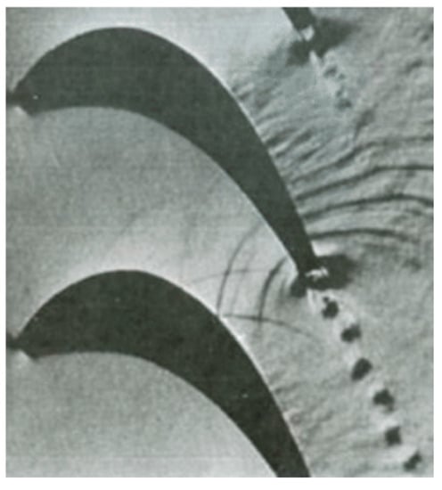
Figure 11.
Schlieren picture of turbine rotor blade wake at [24].
In 1982 Han and Cox [26], performed smoke visualizations on a very large-scale nozzle blade at low speed (Figure 12). The authors found much sharper and well-defined contours of the vortices from the pressure side and concluded that this implied stronger vortex shedding from this side and attributed this to the circulation around the blade.
Figure 12.
Smoke visualization of the vortex shedding from a low speed nozzle blade [26].
Beretta-Piccoli [27] (reported by Bölcs and Sari [28]) was possibly the first to use interferometry to visualize the vortex formation at the blunt trailing edge of a blade at transonic flow conditions.
Besides the problem of time resolution for measuring high frequency phenomena, there was also the problem of spatial resolution for resolving the vortex structures behind the usually rather thin turbine blade trailing edges. First tests on a large scale flat late model simulating the overhang section of a cascade allowed to visualize impressively details of the vortex shedding at transonic outlet Mach number (Figure 13a,b).
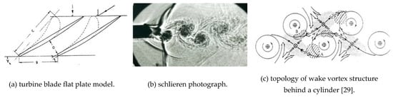
Figure 13.
Vortex shedding at transonic exit flow conditions [30].
Following Hussain and Hayakawa [29], the wake vortex structures can be described by a set of centers which characterize the location of a peak of coherent span-wise vortices and saddles located between the coherent vorticity structures and defined by a minimum of coherent span-wise vorticity. The successive span-wise vortices are connected by ribs, that are longitudinal smaller scale vortices of alternating signs.
A significant progress was made in the 1990’s in the frame of two European Research Projects, i.e., Experimental and Numerical Investigations of Time Varying Wakes behind Turbine Blades (BRITE/EURAM CT-92-0048) and Turbulence Modeling for Unsteady Flows in Axial Turbines (BRITE/EURAM CT-96-0143) in which the von Kármán Institute, the University of Genoa and the ONERA of Lille used short duration flow visualizations and fast response instrumentation in combination with large scale blade models to improve the understanding of the formation of the vortical structures at the turbine blade trailing edges and their impact on the unsteady wake flow characteristics. Results of these research projects are reported by Ubaldi et al. [31], Cicatelli and Sieverding [32], Desse [33], Sieverding et al. [34], Ubaldi and Zunino [35] and Sieverding et al. [21,36].
The large-scale turbine guide vane used in these experiments was designed at VKI (Table 2) and released in 1994 [37]. The blade design features a front-loaded blade with an overall low suction side turning in the overhang section and, in particular, a straight rear suction side from halfway downstream of the throat, Figure 14. Due to mass flow restrictions in the VKI blow down facility, the three-bladed cascade with a chord length mm was limited to investigations at a relatively low subsonic outlet Mach number of . The suction side boundary layer undergoes natural transition at . On the pressure side the boundary layer was tripped at . The boundary layers at the trailing edge with shape factors of 1.64 and 1.41 for the pressure and suction sides respectively, were clearly turbulent. The schlieren photographs in Figure 14 were taken with a Nanolite spark source, with . The dominant vortex shedding frequency was 2.65 kHz and the corresponding Strouhal number, defined as:
was .
Table 2.
VKI LS-94 large scale nozzle blade geometric characteristics [32].
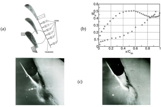
Figure 14.
Very large-scale turbine nozzle guide vane (VKI LS-94); case. (a) test section, (b) surface isentropic Mach number distribution, (c) schlieren photographs. Adapted from [32].
Figure 14c presents two instances in time of the vortex shedding process. The left flow visualization shows the enrolment of the pressure side shear layer into a vortex, the right one the formation of the suction side vortex. Note that the pressure side vortex appears to be much stronger than the suction side one, which confirms the observations made by Han and Cox [26].
Gerrard [38], describes the vortex formation for the flow behind a cylinder as follows, Figure 15. The growing vortex (A) is fed by the circulation existing in the upstream shear layer until the vortex is strong enough to entrain fluid from the opposite shear layer bearing vorticity of the opposite circulation. When the quantity of entrained fluid is sufficient to cut off the supply of circulation to the growing vortex—the opposite vorticity of the fluid in both shear layers cancel each other—then the vortex is shed off.
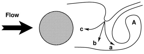
Figure 15.
Vortex formation mechanism; adapted from [38].
Contrary to the blow down tunnel at VKI, the Istituto di Macchine e Sistemi Energetici (ISME) at the University of Genoa used a continuous running low speed wind tunnel. Miniature cross-wire hot-wire probe and a four-beam laser Doppler velocimeter are used for the measurements of the unsteady wake. An example of the instantaneous patterns of the ensemble averaged periodic wake characteristics is presented in Figure 16. A detailed description is given by Ubaldi and Zunino [35]. The streamwise periodic component of the velocity, in Figure 16 (upper left), shows asymmetric periodic patterns of alternating positive and negative velocity components issued from the pressure to the suction side. As already shown schematically in Figure 13, saddle points separating groups of four cores, are located along the wake center line. On the contrary, the periodic parts of the transverse component (upper right) appear as cores of positive and negative values, approximately centered in the wake which alternate, enlarging in streamwise direction. The combination of the two velocity components give rise to the rolling up of the periodic flow into a row of vortices rotating in opposite direction as shown by the velocity vector plots (lower left).
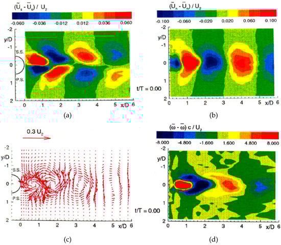
Figure 16.
Instantaneous realization of the ensemble averaged streamwise velocity (a), transversal velocity (b), velocity vector (c) and vorticity patterns (d) of the periodic flow [35].
As illustrated by Gerrard [38] (see Figure 15), the vortex formation is driven by the vorticity in the suction and pressure side boundary layers. The vorticity terms and in the wake have been determined taking respectively the curl of the phase averaged and time averaged velocity field: and , Figure 16 (lower right). The local maxima and minima and saddle regions (the points where the vorticity changes its sign) define the location, extension, rotation and intensity of the vortices.
With increasing downstream Mach number, the vortices become much more intense as demonstrated in Figure 17 on a half scale model of the blade already presented in Figure 14 and Table 2, at an outlet Mach number in a four bladed cascade, Sieverding et al. [36]. Contrary to schlieren photographs which visualize density changes, the smoke visualizations in Figure 17 show the instantaneous flow patterns and are therefore particular well suited to visualize the enrolment of the vortices. A close look at the vortex structures reveals that the distances between successive vortices change. In fact, the distance between a pressure side vortex and a suction side vortex is always smaller than the distance between two successive pressure side vortices. A possible reason is that the pressure side vortex plays a dominant role and exerts an attraction on the suction side vortex as already found by Han and Cox [26].
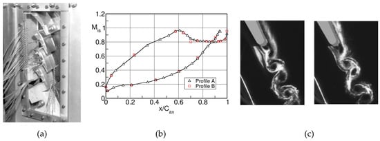
Figure 17.
VKI LS94 turbine blade, case. (a) four blades cascade, (b) surface isentropic Mach number distribution and (c) smoke visualizations. Adapted from [36].
The vortex formation and subsequent shedding is accompanied by large angle fluctuations of the separating shear layers which does not only lead to large pressure fluctuations in the zone of separations but also induces strong acoustic waves. The latter travel upstream on both the pressure and suction side as shown in the corresponding schlieren photographs obtained this time with a continuous light source, a high speed rotating drum and rotating prism camera from ONERA with a maximum frame rate of 35,000 frames per second (see Figure 18), as reported by Sieverding et al. [21].
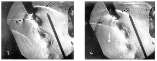
Figure 18.
Schlieren photographs of vortex shedding at two instances in time; [21].
In image 1 of Figure 18 the suction side shear layer has reached its farthest inward position and the local pressure just upstream of the separation point has reached its minimum value. Conversely, on the pressure side the separating shear layer has reached its most outward position. A pressure wave denoted Pi originates from the point where the boundary layer separates from the trailing edge. Upstream of Pi is the pressure wave from the previous cycle. It interferes with the suction side of the neighboring blade from where it is reflected. In image 4 of Figure 18, the suction side shear layer is at its most outward position. A pressure wave originates at the point of separation, denoted Si. The pressure wave further upstream is due to the previous cycle. On the pressure side the pressure wave Pi extends now to the suction side of the neighboring blade. The wave interference point of the previous cycle has moved up-stream. It can therefore be expected that the suction side pressure distribution near the throat region is highly unsteady.
Holographic interferometric density measurements, performed at VKI at by Sieverding et al. [36], give further information about the formation and the shedding process of the von Kármán vortices. The reference density is evaluated from pressure measurements with a fast response needle static pressure probe positioned just outside of the wake assuming the total temperature to be constant outside the wake.
The interferogram in Figure 19 shows the suction side vortex (upper blade surface) in its out most outward position i.e., at the start of the shedding phase. On the pressure side the density patterns point to the start of the formation of a new pressure side vortex. The pressure side vortex of the previous cycle is situated at a trailing edge distance of . This vortex is defined by ten fringes. With a relative density change between two successive fringes of the total relative density change from the outside to the vortex center is . The minimum in the vortex center is compared to an isentropic downstream static to total density ratio of .
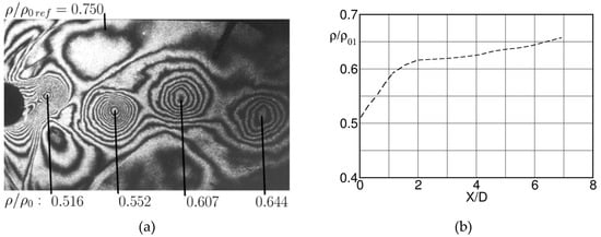
Figure 19.
Instantaneous density distribution (a) and variation of density minima with trailing edge distance (b) at ; adapted from [36].
Based on a large number of tests with holographic interferometry and white light interferometry, see Desse [33], Figure 19 shows the variation of the vortex density minima non-dimensionalized by the upstream total density , in function of the trailing edge distance . There are two distinct regions for the evolution of the vortex minima: a rapid linear density rise-up to distance followed by a much slower rise further downstream.
Comparing the vortex formation at and 0.79 shows that with increasing Mach number the vortices form much closer to the trailing edge. This tendency goes crescendo with further increase of the downstream Mach number as already shown in Figure 13 where normal shocks oscillate close to the trailing edge forward and backward with the alternating shedding of the vortices. A further increase of the outlet flow leads gradually to the formation of an oblique shock system at the convergence of the separating shear layers at short distance behind the trailing edge, causing a delay of the vortex formation to this region as demonstrated by Carscallen and Gostelow [39], in the high speed cascade facility of the NRC Canada. The high speed schlieren pictures revealed some very unusual types of wake vortex patterns as shown in Figure 20. Besides the regular von Kármán vortex street (left), the authors visualized other vortex patterns, such as e.g. couples or doublets, on the right. In other moments in time they observed what they called hybrid or random or no patterns. The schlieren photos in Figure 20 show the existence of an unexpected shock emanating from the trailing edge pressure side at the beginning of the trailing edge circle. Questioning Bill Carscallen [40] recently about the origin of this shock it appeared that the shock was simply due to an inaccuracy in the blade manufacturing of the trailing edge circle.
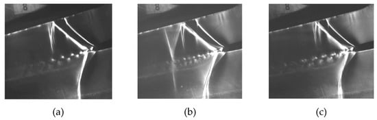
Figure 20.
Occurrence of different vortex patters in wake of transonic blade at . (a) regular vortex street, (b) couples, (c) doublets [39].
The question whether in distinction of the conventional von Kármán vortex street, a double row vortex street of unequal vortex strength may exist, was treated by Sun in 1983 [41]. Figure 21 presents an example of a double row vortex street with unequal vortex strength and vortex distances. The author demonstrated that such configurations are basically unstable.
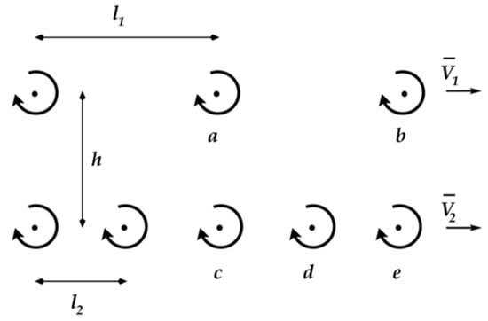
Figure 21.
An example of vortex street with unequal vortex strengths and unequal vortex spacings; adapted from [41].
4. Energy Separation in the Turbine Blade Wakes
In the course of a joint research program between the National Research Council of Canada and Pratt & Whitney Canada of the flow through an annular transonic nozzle guide vane in the 1980s certain experiments revealed a non-uniform total temperature distribution downstream of the uncooled blades, Carscallen and Oosthuizen [42]. Considering the importance of the existence of a non-uniform total temperature distribution at the exit of uncooled stator blade row for the aerothermal aspects of the downstream rotor, the Gasdynamics Laboratory of the National Research Council, Canada decided to build a continuously running suction type large scale planar cascade tunnel (chord length 175.3 mm, turning angle 76°, trailing edge diameter 6.35 mm) and launched an extensive research program aiming at the understanding of the mechanism causing the occurrence of total temperature variations downstream of a fixed blade row, determine their magnitude and evaluate their significance for the design of the downstream rotor. Downstream traverses with copper constantan thermocouples reported by Carscallen et al. [43] in 1996 showed that the total temperature contours correlated perfectly with the total pressure wake profiles, Figure 22.
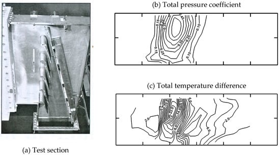
Figure 22.
Total pressure coefficient and temperature contours downstream of a nozzle guide vane at a pressure ratio PR = 1.9; adapted from [42].
In the wake center the total temperature dropped significantly below the inlet total temperature while higher values were recorded near the border of the wake. The differences increased with Mach number and reached a maximum at sonic outlet conditions. The question was then to elucidate the reasons for these temperature variations. The research on flows across cylinders was already more advanced in this respect. Measurements of the temperature distribution around a cylinder for a flow normal to the axis of the cylinder, performed at the Aeronautical Institute of Braunschweig in the late 1930’s and reported by Eckert and Weise [44] in 1943, showed that the recovery temperature at the base of the cylinder reduced below the true (static) temperature of the incoming flow, so that the recovery factor:
attained negative values in the base region (see Figure 23).
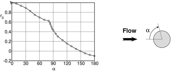
Figure 23.
Evolution of the recovery factor in the azimuthal direction from the stagnation point (°) to the rear side of the cylinder (); adapted from [44].
The authors suspected that the low values were possibly due to the intermittent separation of vortices from the cylinder. These results were confirmed by Ryan [45] in 1951 at Ackeret’s Institute in Zürich who clearly related this low temperature to the periodic vortex shedding behind the cylinder as cause for the energy separation in the fluctuating wake. He also noticed that the energy separation was particularly large when a strong sound was generated by the flow.
The existence of a low temperature field at the base of a cylinder was also observed by Sieverding in 1985, who used an infrared camera to visualize through a germanium window in the side wall of a blow down wind tunnel the wall temperature field around a 15 mm diameter cylinder at , see Figure 24. Unfortunately, due to a lack of time it was not possible to determine the absolute temperature values.
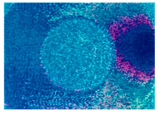
Figure 24.
Side wall temperature field around a cylinder recorded by an infrared camera.
Eckert [46] explained the mechanism of energy separation along a flow path with the help of the unsteady energy equation:
The change of the total temperature with time depends on: (a) the partial derivative of the pressure with time, (b) on the energy transport due to heat conduction between regions of different temperatures and (c) on the work due to viscous stresses between regions of different velocities. As regards the flow behind bluff bodies the two latter terms are considered small compared the pressure gradient term and Equation (4) then reduces to:
The occurrence of total temperature variations in the vortex streets behind cylinders was e.g. extensively described by Kurosaka et al. [47], Ng et al. [48] and Sunduram et al. [49].
The progress in the understanding of the mechanism was boosted with the arrival of fast temperature probes as for example the dual sensor thin film platinum resistance thermometer probe developed by Buttsworth and Jones [50] in 1996 at Oxford. Using their technique Carscallen et al. [51,52] were the first to measure the time varying total pressure and temperature in the wake of their turbine vane. Figure 25 presents the results for an isentropic outlet Mach number and a vortex shedding frequency of the order of 10 kHz. The probe traverse plane was normal to the wake at a distance of 5.76 trailing edge diameters from the vane trailing edge. In a later paper concerning the same cascade, Gostelow and Rona [53], published also the corresponding entropy variations from the Gibb’s relation:
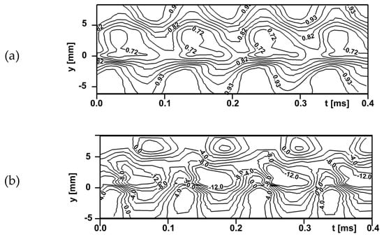
Figure 25.
Contour plots of phase averaged total pressure (a) and total temperature (b) behind turbine vane; adapted from [51].
The results are presented in Figure 26.
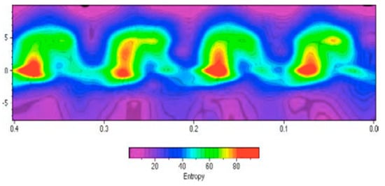
Figure 26.
Time resolved measurements of entropy increase [53].
The variation of the maxima and minima of the total temperature in the center of the wake vary between a minimum of −15° to a maximum of −4° with respect to the inlet ambient temperature, Figure 27. At the border of the wake the temperature raises considerably above the inlet temperature, while the time averaged temperature in the wake center is about −10°.
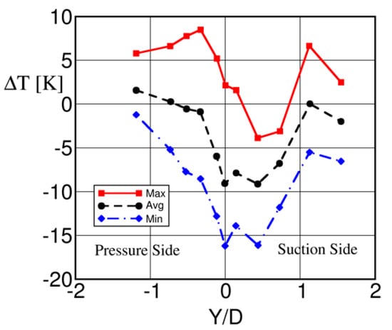
Figure 27.
Variation of total temperature maxima and minima through the wake; adapted from [51].
In 2004, Sieverding et al. [36] published very similar results for the turbine vane shown in Figure 17. The wake traverse was performed at a trailing edge distance of only in direction of the tangent to the blade camber line, which forms an angle of 66° with the axial direction. The traverse is made normal to this tangent.
The steady state total pressure and total temperature measurements are presented in Figure 28. Similar to the results obtained at the NRC Canada, the wake center is characterized by a pronounced total temperature drop of 3% of the inlet value of 290 K which corresponds to about −9°, a variation which is of the same order as that reported in Figure 27. On the borders of the wake, total temperature peaks in excess of the inlet temperature are also recorded. The mass integrated total temperature value across the wake (denoted with a ) should be such that <, but lack of information on the local velocity did not allow to perform this integration.
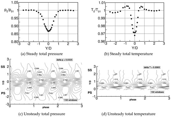
Figure 28.
Steady and time varying phase lock averaged total pressure and total temperature through turbine vane wake at ; adapted from [36].
For the measurement of the time varying temperature a fast 2 μm cold wire probe, developed by Denos and Sieverding [54], was used. Numerical compensation allowed to extend the naturally low frequency response of the probe to much higher ranges for adequate restitution of the nearly sinusoidal temperature variation associated with the vortex shedding frequency of 7.6 kHz at a downstream isentropic Mach number of . As regards the total pressure variation , minimum values of 0.768 are reached in the wake center while at the wake border maximum values of 1.061 are recorded. As regards the total temperature the authors quote maximum and minimum total temperature ratios of and , respectively. With a the maximum total temperature variations are of the order of 24°, similar to those reported by Carscallen et al. [51]. However, the flow conditions were different: at VKI, versus 0.95 at NRC Canada, and a distance of the wake traverses with respect to the trailing edge of 2.5 diameters at VKI, versus 5.76 at NRC.
5. Effect of Vortex Shedding on Blade Pressure Distribution
The previous section focused on the unsteady character of turbine blade wake flows, the visualization of the von Kármán vortices through smoke visualizations, schlieren photographs and interferometric techniques. The measurement of the instantaneous velocity fields using LDV and PIV techniques allowed to determine the vorticity distribution and the measurement of the unsteady total pressure and temperature distribution putting into evidence the energy separation effect in the wakes due to the von Kármán vortices.
Naturally the vortex shedding affects also the trailing edge pressure distribution and, beyond that, the suction side pressure distribution. The following is entirely based on research work carried out at the VKI by the team of the lead author, who was the only one to measure with high spatial resolution the pressure distribution around the trailing edge of a turbine blade.
5.1. Effect on Trailing Edge Pressure Distribution
The very large-scale turbine guide vane designed and tested at the von Kármán Institute with a trailing edge thickness of 15 mm did allow an innovative approach for obtaining a high spatial resolution for the pressure distribution around the trailing edge. Cicatelli and Sieverding [32], fitted the blade with a rotatable 20 mm long cylinder in the center of the blade (Figure 29). The cylinder was equipped with a single Kulite fast response pressure sensor side by side with an ordinary pneumatic pressure tapping. The pressure sensor was mounted underneath the trailing edge surface with a slot width of only 0.2 mm to the outside, the same width as the pressure tapping, reducing the angular sensing area to only 1.53°. To control any effect of the rear facing step between the blade lip and the rotatable trailing edge, a second blade was equipped with additional pressure sensors placed at, and slightly up-stream of, the trailing edge.
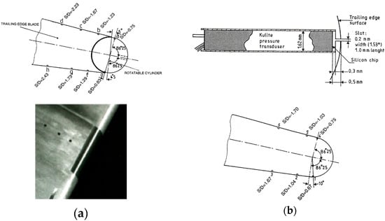
Figure 29.
Blade instrumented with rotatable trailing edge (a: blade A) and control blade (b: blade B); adapted from [32].
The time averaged base pressure distribution, non-dimensionalized by the inlet total pressure, is presented in Figure 30. The circles denote data obtained with the rotatable trailing edge cylinder on blade A, while the triangles are measured with pressure tappings on blade B (see Figure 29), except for the two points “a” and “e” which are taken from the pressure tappings positioned aside the rotating cylinder on blade A (see Figure 30, left panel). The flow approaching the trailing edge undergoes, both on the pressure and suction side, a strong acceleration before separating from the trailing edge circle. The authors attribute the asymmetry to differences in the blade boundary layers and to the blade circulation, which, following Han and Cox [26], strengthens the pressure side vortex shedding. Compared to the downstream Mach number , the local peak numbers are as high as and 0.47, respectively. These high over-expansions are incompatible with a steady state boundary layer separation and are attributed to the effect of the vortex shedding.
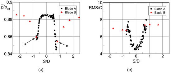
Figure 30.
Phase lock averaged trailing edge pressure distribution (a) and root mean square values of the pressure fluctuations (b) for the VKI turbine blade at ; adapted from [32].
Figure 30, right panel, presents the corresponding root mean square of the pressure signal. Maximum pressure fluctuations of the order of 8% occur near the locations of the pressure minima, i.e., close to the boundary layer separation points, while the RMS/Q drops to nearly half this value in the central region of the trailing edge base. It is also worth noting that the pressure fluctuations affect also the flow upstream of the trailing edge. In the center of the base region there is an extended constant pressure plateau (Figure 30). The base pressure coefficient corresponding to this plateau agrees well with the Sieverding’s base pressure correlation.
The base pressure distribution changes dramatically at high subsonic downstream Mach numbers as illustrated by Sieverding et al. [21], Figure 31. The pressure distribution is characterized by the presence of three minima: the two pressure minima associated with the over-expansion of the suction and pressure side flows before separation from the trailing edge, and an additional minimum around the center of the trailing edge circle. The pressure minima related to the overexpansion from suction and pressure sides are of the order of for both sides, i.e., the local peak Mach numbers are close to 1. Contrary to the low Mach number flow condition of Figure 30, the recompression following the over-expansion does not lead to a pressure plateau but gives way to a new strong pressure drop reaching a minimum of at +7°. This is the result of the enrolment of the separating shear layers into a vortex right at the trailing edge; the vortex core approaches the wake centerline and its distance to the trailing edge becomes less than half the trailing edge diameter, see smoke visualization and interferogram in Figure 17 and Figure 19.
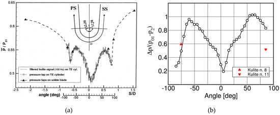
Figure 31.
Steady state trailing edge pressure distribution (a) and phase locked average pressure fluctuation (b) around trailing edge; adapted from [21].
The phase lock averaged pressure fluctuations around the trailing edge in Figure 31 are impressive. They are naturally highest near the separation points of the boundary layer from the trailing edge where maximum values of around 100% of the dynamic pressure () are recorded. The minimum pressure in a given position corresponds to the maximum inward motion of the separating shear layer, the maximum pressure to the maximum outward motion of the separating shear layer. The maximum local instantaneous Mach number at the point of the most inward position can be as high as . The authors assumed that the curvature driven supersonic trailing edge expansion is the real reason for the formation of the vortex so close to the trailing edge, with the entrainment of high-speed free stream fluid into the trailing edge base region. In the center of the trailing edge the fluctuations drop to 20% of the dynamic head.
The authors provide also some interesting information on the evolution of the pressure signal on the trailing edge circle over one complete vortex shedding cycle. This is demonstrated in Figure 32 showing the evolution for the phase locked average pressure at the angular position of 60° on the pressure side of the trailing edge circle. A decrease of the pressure indicates an acceleration of the flow around the trailing edge i.e., the separating shear layer moves inwards, the vortex is in its formation phase. An increase of the pressure indicates on the contrary an outwards motion of the shear layer, the vortex is in its shedding phase. Surprisingly, the pressure rise time is much shorter than the pressure fall time, i.e., the time for the vortex formation is longer than that for the vortex shedding. The same was observed for the pressure evolution on the opposite side of the trailing edge, but of course with 180° out of phase.
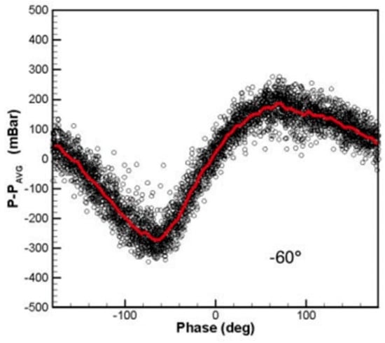
Figure 32.
Phase locked average pressure variation at trailing edge at an angular position of −60° [21].
The change of an isobaric pressure zone over an extended region at the base of the trailing edge at an exit Mach number to a highly non-uniform pressure distribution with a strong pressure minimum at the center of the trailing edge circle at , did of course raise the question about the evolution of the trailing edge pressure distribution over the entire Mach number range, from low subsonic to transonic Mach numbers. To respond to this lack of information a research program was carried out by Mateos Prieto [55] at VKI as part of his diploma thesis in 2003. For various reasons, the data were not published at that time but only in 2015, as part of the paper of Vagnoli et al. [56] on the prediction of unsteady turbine blade wake flow characteristics and comparison with experimental data, see Figure 33.
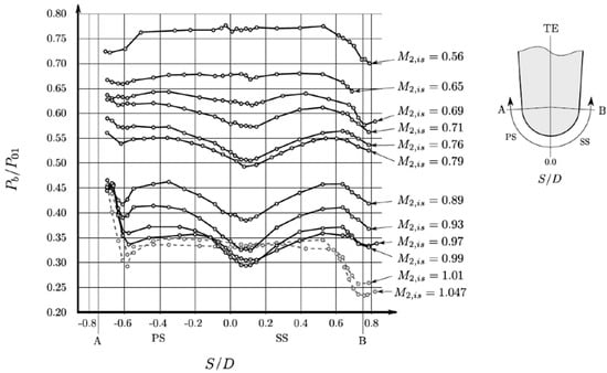
Figure 33.
Effect of downstream Mach number on trailing edge Mach number distribution [56].
The figure puts clearly into evidence the effect of the vortex shedding on the trailing edge pressure distribution. Up to about the trailing edge base region is characterized by an extended, nearly isobaric, pressure plateau which implies that the vortex formation occurs sufficiently far downstream not to affect the trailing edge base region. With increasing Mach number, the enrolment of the shear layers into vortices occurs gradually closer to the trailing edge causing an increasingly non-uniform pressure distribution with a marked pressure minimum at the center of the trailing edge. To characterize the degree of non-uniformity the authors define a factor :
where is the maximum pressure following the recompression after the separation of the shear layer from the trailing edge and the minimum pressure near the center of the trailing edge. The maximum degree of non-uniformity is reached at with a value of 21%. At this Mach number the minimum pressure reaches a value of for a downstream pressure . With further increase of the Mach number, starts to decrease rapidly. It decreases to = 12% at and drops to zero at . For this Mach number the local trailing edge conditions are such that oblique shocks emerge from the region of the confluence of the suction and pressure side shear layers and the vortex formation is delayed to after this region as shown e.g. in the schlieren picture by Carscallen and Gostelow [39] at the NRC Canada in Figure 34, left, and another schlieren picture taken at VKI in Figure 34, right (unpublished).
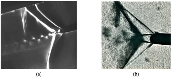
Figure 34.
At fully established oblique trailing edge shock system the vortex formation is delayed to after the point of confluence of the blade shear layers. NRC blade (a) [39], VKI blade (b).
As already pointed out at the end of Section 2 the departure from the generally assumed isobaric trailing edge base region may explain the differences of base pressure data published by different authors at high subsonic/transonic downstream Mach numbers. The scatter between experimental data from different research organizations may be partially due to the use of very different ratios of the diameter of the trailing edge pressure hole to the trailing edge diameter, . Small ratios may lead to an overestimation of the base pressure effect. Hence, base pressure measurements should be taken with a ratio as large as possible.
The existence of an isobaric base pressure region for supersonic trailing edge flows, i.e., for blades with a well-established oblique trailing edge shock system as those in Figure 34, was already known from flat plate model tests simulating the overhang section of convergent turbine blades with straight rear suction side since 1976 [18], see Figure 35. The tests were performed for a gauging angle . The inclination of the tail board attached to the lower nozzle block allows to increase the downstream Mach number which entails of course the displacement of the suction side shock boundary interaction along the blade suction side towards the trailing edge.
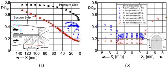
Figure 35.
Surface (a) and trailing edge (b) pressure distribution for flat plate model tests; adapted from [18].
The schlieren photograph on the right in Figure 34 shows the occurrence of so-called lip shocks at the separation of the shear layers from the trailing edge due to a slight overturning and a non-tangential separation of the flow from the trailing edge surface. In a later test series with a denser instrumentation of the trailing edge, Sieverding et al. [4] showed that the trailing edge shock strength was however weak. In Figure 36 the pressure increase across the lip shock is presented in function of the expansion ratio around the trailing edge , where is the pressure before the start of the expansion around the trailing edge and the pressure before the lip shock. All data are within a bandwidth of .
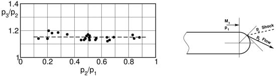
Figure 36.
Strength of the trailing edge lip shocks; adapted from [4].
Raffel and Kost [57] performed similar large-scale tests on a flat plate with a slotted trailing edge to investigate the effect of trailing edge blowing on the formation of the trailing edge vortex street. Their trailing edge pressure distributions taken at zero coolant flow ejection for downstream Mach numbers of confirm the existence of an isobaric pressure trailing edge base region, but the measurements are unfortunately not dense enough to extract consistent data about the strength of the lip shock. A few data allow to conclude that in their experiments the maximum lip shock strength is of the order of .
5.2. Effect on Blade Suction Side Pressure Distribution
In the discussion of the schlieren photographs in Figure 18 it was shown that the outwards motion of the oscillating shear layers at the blade trailing edge does not only lead to large pressure fluctuations in the zone of separations, but it does also induce strong acoustic pressure waves travelling upstream on both the suction and pressure side of the blade. To facilitate the understanding of the suction side pressure fluctuations in Figure 37, the left photo of the schlieren pictures in Figure 18 is reproduced at the right of the pressure curves. The wave Pi generated at the pressure side will interact with the suction side of the neighboring blade causing significant unsteady pressure variations as measured by fast response pressure sensors implemented between the throat and the trailing edge of this blade, see Figure 37. The pressure wave induced by the outwards motion of the pressure side shear layer of the neighboring blade intersects the suction side between the sensors 3 and 4. It moves then successively upstream across the sensors 3 and 2. The signals are asymmetric, characterized by a sharp pressure rise followed by a slow decay. The amplitude of the pressure fluctuations is important with up to of () at sensor 3, and at sensor 2, while the pressure signal is flat at sensor 1 situated slightly up-stream of the geometric throat where the blade Mach number reaches . The pressure waves observed at sensor 4 and further downstream at sensors 5 and 6 are more sinusoidal in nature and of smaller amplitude. The authors suggested that these fluctuations are likely to be caused by the downstream travelling vortices of the neighboring blade.
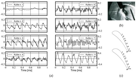
Figure 37.
Unsteady pressure variations along rear suction side (a); schlieren photograph (b); kulite sensor positioning (c). Adapted from [21].
The periodicity of the pressure signal at position 7, slightly upstream of the trailing edge, is rather poor and only phase lock averaging provides useful information on its periodic character. The reason is most likely the result of a superposition of waves induced by the von Kármán vortices in the wake of the neighboring blade and upstream travelling waves induced by the oscillation of the suction side shear layer designated by “S” in the schlieren photographs. Right at the trailing edge, position 11, we have, as expected, strong periodic signals associated with the oscillating shear layers.
6. Turbine Trailing Edge Vortex Frequency Shedding
Besides the importance of trailing edge vortex shedding for the wake mixing process and the trailing edge pressure distribution discussed before, vortex shedding deserves also special attention due to its importance as excitation for acoustic resonances and structural vibrations. Heinemann & Bütefisch [25], investigated 10 subsonic and transonic turbine cascades: two flat plate turbine tip sections, three mid-sections with nearly axial inlet (one blade tested with three different trailing edge thicknesses) and 3 high turning hub sections. The trailing edge thickness varied from 0.8% to 5%. The vortex shedding frequency was determined with an electronic-optical method developed at the DFVLR-AVA by Heinemann et al. [58].
The corresponding Strouhal numbers defined in (3) covered a wide range: for a Reynolds number range based on trailing edge thickness and downstream isentropic velocity of . The Strouhal numbers for flows from cylinders over the same Reynolds number range are of the order of and 0.21 as shown in Figure 38.
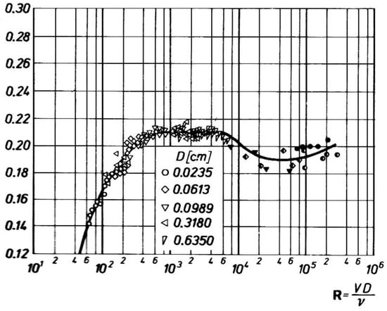
Figure 38.
Strouhal numbers in sub-critical Reynolds number range for flow over cylinders; adapted from [59].
Figure 39 presents the Strouhal numbers for 3 of the 10 turbine blade sections investigated by Heinemann and Bütefisch [25]. The comparison with the flow across cylinders is limited to the subsonic range. The Strouhal numbers for the flat plate tip section T2 are of the order of = 0.2 in the Mach range = 0.2 to 0.8 and therewith very close to the those of the flow over cylinders. On the other side, the hub section H2 with a high rear suction side curvature distinguishes itself by Strouhal numbers as high as 0.38 − 0.3, with a decreasing tendency from = 0.2 to 0.9. For the mid-section M2 with low rear suction side turning, the authors report Strouhal numbers increasing from = 0.22 to 0.29 for a Mach range 0.2 to 0.8.
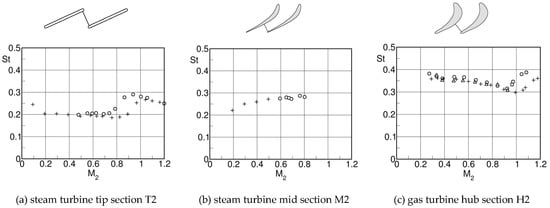
Figure 39.
Strouhal number for 3 blade sections.  : and based on isentropic downstream velocity. : and based on homogeneous downstream velocity. Adapted from [25].
: and based on isentropic downstream velocity. : and based on homogeneous downstream velocity. Adapted from [25].
Additional information on turbine blade trailing edge frequency measurements were published by Sieverding [60] who used fast response pressure sensors implemented in the blade trailing edge and in a total pressure probe positioned at short distance from the trailing edge, while Bryanston-Cross and Camus [61] made use of a 20 MHz bandwidth digital correlator combined with conventional schlieren optics. The Strouhal numbers of Sieverding’s rotor blade with a straight rear suction side were in the lower part of the band width of the DFVLR-AVA data, while those of Bryanston-Cross and Camus rotor blades with higher suction side curvature resided in the upper part.
The large range of Strouhal numbers were possibly due to differences in the state of the boundary layers at the point of separation. Besides that, the vortex shedding frequency does not simply depend on the trailing edge thickness augmented by the boundary layer displacement thickness, which, however, is in general not known, but rather on the effective distance between the separating shear layers which could be significantly smaller than the trailing edge thickness. Patterson & Weingold [62], simulating a compressor airfoil trailing edge flow field on a flat plate, concluded that, compared to the effective distance between the separating upper and lower shear layers, the state of the boundary layer before separation played a much more important role.
The influence of the boundary layer state and of the effective distance of the separating shear layers was specifically addressed in a series of cascade and flat plate tests investigated by Sieverding & Heinemann [16], at VKI and DLR. Figure 40 shows the blade surface isentropic Mach number distributions of a front loaded blade, with the particularity of a straight rear suction side (blade A), and a rear loaded blade (blade C), characterized by a high rear suction side turning angle, at a downstream Mach number of .
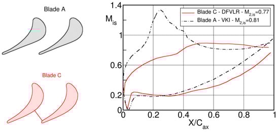
Figure 40.
Blade Mach number distributions for front and rear-loaded blades; adapted from [16].
The early suction side velocity peak on blade A will cause early boundary layer transition. On the contrary, considering the weak velocity peak on the rear suction side followed by a very moderate recompression, the suction side boundary layer of blade C is likely to be laminar at the trailing edge over a large range of Reynolds numbers. As regards the pressure sides of both blades, the strong acceleration over most part of the surface is likely to guarantee laminar conditions at the trailing edge on both blades and trip wires had to be used to enforce transition and turbulent boundary layers at the trailing edge, if desired so. The blades were tested from low subsonic to high subsonic outlet Mach numbers. Due to the use of blow down and suction tunnels at VKI and DLR, respectively, the Reynolds number increases with Mach number as shown in Figure 41.
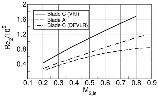
Figure 41.
Variation of Reynolds number in function of downstream Mach number; adapted from [16].
The tests for the front-loaded blade A are presented in Figure 42. In case of forced transition on the pressure side through a trip wire at 24% of the chord length, the Strouhal number is nearly constant and roughly equal to over the entire Mach range. In absence of a trip wire, the evolution of is quite different. Starting from the low Mach number and Reynolds number end, the Strouhal number decreases from at to at . At this point the drops suddenly to the level of all turbulent cases. This sudden change obviously indicates that boundary layer transition has taken place on the pressure side. The slow decrease before the sudden jump points to a progressive change from a laminar to a transitional boundary layer which is obviously related to the increasing Reynolds number.
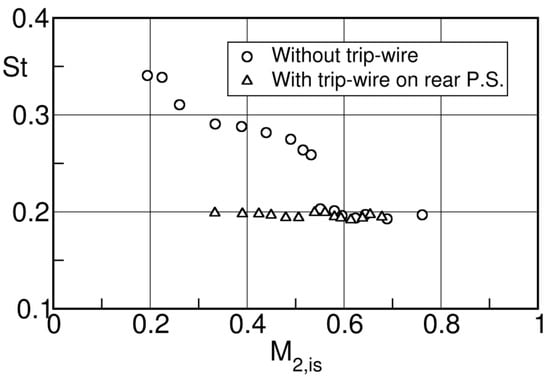
Figure 42.
Strouhal number variation with downstream Mach number for cascade A; adapted from [16].
Cascade C was tested with a circular trailing edge at DLR and a squared trailing edge at VKI over a range = 0.2 to 0.9. The two series of test differed not only by their trailing edge geometry but also, at the same Mach number, by a higher Reynolds number in the VKI tests, see Figure 41. Note, that in the case of the squared trailing edge the distance between the separating shear layers is well defined. However, this is not the case for the rounded trailing edge in which case the distance should be in any way smaller. But one single test, at = 0.59, was run at VKI also with a rounded trailing edge to eliminate any bias between the tests at DLR and VKI.
Figure 43 presents the Strouhal number for blade C both in function of the downstream Mach number and the Reynolds number. Both data sets show a plateau of at low Mach number and Reynolds number which is characteristic for a fully laminar trailing edge boundary layer separation. The Strouhal number starts to decrease with increasing Reynolds number, the drop of occurring earlier at for the squared trailing edge, instead of for the circular trailing edge. At the squared trailing edge data reach a plateau with . Note that the single rounded trailing edge test at VKI indicated by a star in the graph is right in line with the squared trailing edge data. Extrapolating the DLR data to higher Reynolds number one may expect that they will reach the plateau of = 0.24 at .
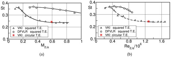
Figure 43.
Strouhal number variation with Mach number (a) and Reynolds number (b) for cascade C; adapted from [16].
Comparing the two curves in Figure 43 raises of course the question as to the reasons for the differences between them. The possible influence of the different distance between the separating shear layers was already mentioned before, but, if this would be the case, then the Strouhal number for the VKI tests with squared trailing edge should be higher than those of the DLR tests with rounded trailing edge. There must be therefore a different reason. The key for the understanding comes from flat plate tests presented in [16], see Figure 44, which showed that the difference of the Strouhal number between a full laminar and full turbulent flow conditions was much bigger for tests with rounded trailing edges than squared trailing edges, 30% instead of 13%.
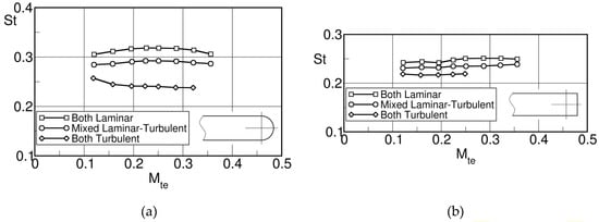
Figure 44.
Strouhal numbers for vortex shedding from flat plates with rounded (a) and squared (b) trailing edges; adapted from [16].
This different behavior can be explained if one assumes that the shape of the trailing edge may strongly affect the evolution of the shear layer, and that it is the state of the shear layer rather than that of the boundary layer which plays the most important role in the generation of the vortex street. Of course, a sharp corner will not necessarily induce immediately full transition, but transition will occur over a certain length, and this length affects the length of the enrolment of the vortex and therewith its frequency. The transition length of the shear layer will be affected by both the Reynolds number and the Mach number.
Contrary to the vortex shedding for subsonic flow conditions discussed above, where the vortices are generated by the enrolment of the separating shear layers close to the blade trailing edge, the situation changes with the emergence of oblique shocks from the region of the confluence of the pressure and suction side shear layers for transonic outlet Mach numbers. In this case the vortex formation is delayed to after this region as shown already in the schlieren pictures in Figure 34.
This is even more clearly demonstrated in Figure 45 presenting the evolution of the wake density gradients predicted with a LES by Vagnoli et al. [56], for the turbine blade shown in Figure 17, from high subsonic to low supersonic outlet Mach numbers. For the vortex shedding frequency is not any more conditioned by the trailing edge thickness but by the distance between the feet of the trailing edge shocks emanating from the region of the confluence of the two shear layers.
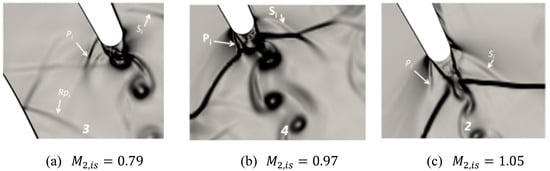
Figure 45.
Change of wake density gradients from subsonic to supersonic exit Mach numbers as predicted by LES [56].
Consequently, one observes a sudden increase of the vortex shedding frequency as for example recorded by Carscallen et al. [43], on their nozzle guide vane, see Figure 46.
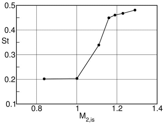
Figure 46.
Strouhal number versus downstream Mach number; adapted from [43].
7. Advances in the Numerical Simulation of Unsteady Turbine Wake Characteristics
The numerical simulation of unsteady turbine wake flow is relatively young, and the first contributions appeared in the mid-80s. The decade 1980–1990 has in fact seen the final move from the potential flow models to the Euler and Navier-Stokes equations whose numerical solutions were tackled with new, revolutionary for the time, techniques. Those were also the years of the first vector and parallel super-computers capable of a few sustained gigaflops (CRAY YMP, IBM SP2, NEC SX-3, to quote a few examples), and of the beginning of the massive availability of computing resources obeying Moore’s law (transistor count doubling every two years). Since then the progresses have been huge both on the numerical techniques and on the turbulence modelling side. Indeed, the most advanced option, that is the Direct Numerical Simulation (DNS) approach, where all turbulent scales are properly space-time resolved down to the dissipative one, has also recently entered the turbomachinery community starting from the pioneering work of Jan Wissink in 2002 [63]. Unfortunately, because of the very severe resolution requirements, there is still no DNS study of turbine wake flow (TWF) at realistic Reynolds and Mach numbers, that is Re ~ and high subsonic and transonic outlet Mach numbers with shocked flow conditions, although improvements have been recently attained [64]. With the development of highly parallelizable codes and the help of very large-scale computing hardware such a simulation is likely to appear soon, as the result of some cutting-edge scientific research. In the meantime, and within the foreseeable future, the industrial world and the designers interested in tangled aspects of TWF for stage performance enhancement will certainly run unsteady flow simulations where turbulence is handled through advanced modeling. Many of those simulations will rely on in-house developed research codes and turbomachinery oriented commercial packages, which, indeed, have improved significantly since the very first unsteady TWF simulation. Yet, there are two areas where important challenges still need to be satisfactorily faced before the presently available (lower fidelity) computations could be considered reliable and successful. They can be, loosely speaking, termed of numerical and modeling nature. We shall try to review both, in the context of the presently discussed unsteady turbine wake flow subject category, presenting a short overview of the available technologies. A more specialized review study on high-fidelity simulations as applied to turbomachinery components has recently been published by Sandberg et al. [65].
7.1. Numerical Aspects
Most of the available turbine wake flow computations have been obtained with eddy viscosity closures and structured grid technologies, although a few examples documenting the use of fully unstructured locally adaptive solvers are available [66,67]. In the structured context turbomachinery blades gridding is considered a relatively simple problem, and automated mesh generators of commercial nature producing appreciable quality multi-block grids, are available [68]. The geometrical factors most affecting the grid smoothness are the cooling holes, the trailing edge shape, the sealing devices and the fillets. Of those the trailing edge thickness and its shape are the most important in TWF computations. Low and intermediate pressure turbines (LPT and IPT, respectively) have relatively sharp trailing edges, while the first and second stages of the high-pressure turbines (HPT), often because of cooling needs, have thicker trailing edges. Typically, the trailing edge thickness to chord ratio , is a few percent in LPTs and IPTs, and may reach values of 10% or higher in some HPTs. Thus, the ratio of the trailing edge wet area to the total one may easily range from 1/200 to 1/20, having roughly estimated the blade wet area as twice the chord. Therefore, resolving the local curvature of the trailing edge area is extremely demanding in terms of blade surface grid, that is, in number of points on the blade wall. Curvature based node clustering may only partially alleviate this problem. In addition, preserving grid smoothness and orthogonality in the trailing edge area is difficult, if not impossible with H or C-type grids, even with elliptic grid generators relying on forcing functions [69]. Wrapping an O-type mesh around the blade is somewhat unavoidable, and in any event the use of a multi-block or multi-zone meshing is highly desirable. Unstructured hybrid meshes would also typically adopt a thin O mesh in the inner wall layer. Non-conformal interfaces of the patched or overlapped type would certainly enhance the grid quality, at the price of additional computational complexities and some local loss of accuracy occurring on the fine-to-coarse boundaries [70]. Local grid skewness accompanied by a potential lack of smoothness will pollute the numerical solution obtained with low-order methods, introducing spurious entropy generation largely affecting the features of the vortex shedding flow. In those conditions, the base pressure is typically under-predicted as a consequence of the local flow turning and separation mismatch, with a higher momentum loss and an overall larger unphysical loss generation in the far wake. The impact of those grid distorted induced local errors on the quality of the solution is hard to quantitatively ascertain both a-priori and a-posteriori, and often grid refinement will not suffice, as they frequently turn out to be order 1, rather than order with the mesh size and the order of accuracy. Nominally second order schemes have in practice . In this context, higher order finite difference and finite volume methods, together with the increasingly popular spectral-element methods, offer a valid alternative to standard low order methods [71,72,73,74,75]. This is especially true for those techniques capable of preserving the uniform accuracy over arbitrarily distorted meshes, a remarkable feature that may significantly relieve the grid generation constraints, besides offering the opportunity to resolve a wider range of spatial and temporal scales with a smaller number of parameters compared to the so called second order methods (rarely returning on curvilinear grids). The span of scales that needs to be resolved and the features of the coherent structures associated to the vortex shedding depend upon the blade Reynolds number, the Mach number (usually built with the isentropic downstream flow conditions) and the ratio. This is equivalent to state that the Reynolds number formed with the momentum thickness of the turbulent boundary layer at the trailing edge () and the Reynolds number defined using the trailing edge thickness (), are independent parameters. For thick trailing edge blades the vortex shedding is vigorous and the near wake development is governed by the suction and pressure side boundary layers which differ. Thus, the early stages of the asymmetric wake formation chiefly depend upon the local grid richness, the resolution of the turbulent boundary layers at the TE and the capabilities of the numerical method to properly describe their mixing process. Well-designed turbine blades operate with an equivalent diffusion factor smaller than 0.5 yielding a ratio less than 1% according to Stewart correlation [76]. This effectively means that the resolution to be adopted for the blade base area will have to scale like the product × which may be considerably less than one; in order words the base area region needs more points that those required to resolve the boundary layers at the trailing edge. Very few simulations have complied with this simple criterion as today.
Compressibility effects present additional numerical difficulties, especially in scale resolving simulations. It is a known fact that transonic turbulent TWF calculations require the adoption of special numerical technologies capable to handle time varying discontinuous flow features like shock waves and slip lines without affecting their physical evolution. Unfortunately, most of the numerical techniques with successful shock-capturing capabilities rely on a local reduction of the formal accuracy of the convection scheme whether or not based on a Riemann solver. Since at grid scale it is hard to distinguish discontinuities from turbulent eddies, and even more their mutual interaction, Total Variation Diminishing (TVD) and Total Variation Bounded (TVB) schemes [77,78,79] are considered too dissipative for turbulence resolving simulations, and they are generally disregarded. At present, in the framework of finite difference and finite volume methods, there is scarce alternative to the adoption of the class of ENO (Essentially Non Oscillatory) [80,81,82] and WENO (Weighted Essentially Non Oscillatory) [83,84,85,86,87] schemes developed in the 90s. A possibility is offered by the Discontinuous Galerkin (DG) methods [88]. The DG is a relatively new finite element technique relying on discontinuous basis functions, and typically on piecewise polynomials. The possibility of using discontinuous basis functions makes the method extremely flexible compared to standard finite element techniques, in as much arbitrary triangulations with multiple hanging nodes, free independent choice of the polynomial degree in each element and an extremely local data structure offering terrific parallel efficiencies are possible. In their native unstructured framework, opening the way to the simulation of complex geometries, h and p-adaptivity are readily obtained. The DG method has several interesting properties, and, because of the many degrees of freedom per element, it has been shown to require much coarser meshes to achieve the same error magnitudes when compared to Finite Volume Methods (FVM) and Finite Difference Methods (FDM) of equal order of accuracy [89]. Yet, there seem to persist problems in the presence of strong shocks requiring the use of advanced non-linear limiters [90] that need to be solved. This is an area of intensive research that will soon change the scenario of the available computational methods for high fidelity compressible turbulence simulations.
7.2. Modeling Aspects
The lowest fidelity level acceptable for TWF calculations is given by the Unsteady Reynolds Averaged Navier-Stokes Equations (URANS) or, better, Unsteady Favre Averaged Navier-Stokes Equations (UFANS) in the compressible domain. URANS have been extensively used in the turbomachinery field to solve blade-row interaction problems, with remarkable success [91,92]. The pre-requisite for a valid URANS (here used also in lieu of UFANS) is that the time scale of the resolved turbulence has to be much larger than that of the modeled one, that is to say the characteristic time used to form the base state should be sufficiently small compared to the time scale of the unsteady phenomena under investigation. This is often referred to as the spectral gap requirement of URANS [93]. Therefore, we should first ascertain if TWF calculations can be dealt with this technology, or else if a spectral gap exists. The analysis amounts at estimating the characteristic time , or frequency , of the wake vortex shedding, and compare it with that of the turbulent boundary layer at the trailing edge, l, or . The wake vortex shedding frequency is readily estimated from:
which has been shown to depend upon the turbine blade geometry and the flow regimes (see Figure 39, Figure 42, Figure 43, Figure 44 and Figure 46). For the turbulent boundary layers the characteristic frequency can be estimated, using inner scaling variables, as:
with the friction velocity, and the kinematic viscosity. Assuming the boundary layer to be fully turbulent from the leading edge, and using the zero pressure gradient incompressible flat plate correlation of Schlichting [59]:
one gets:
At the turbine trailing edge , and so that:
Therefore, the ratio of the turbulent boundary layer characteristic frequency to the wake vortex shedding one is, roughly:
The explicit dependence of the Strouhal number upon the geometry term is unknown, although clear trends have been highlighted in the previous section. However, taking and as reasonable values, Equation (6) returns:
The estimates obtained from the above Equation are reported in Table 3, for a few Reynolds numbers.
Table 3.
Turbulent boundary layer to vortex shedding frequency ratio; Equation (7).
From the above table it is readily inferred that, for the problem under investigation, a neat spectral gap exists, and, thus, URANS calculations can be carried out with some confidence. The results reported in the foregoing confirm that this is indeed the case.
Formally, RANS are obtained from URANS dropping the linear unsteady terms, and, therefore, the closures developed for the steady form of the equations apply to the unsteady ones as well. Whether the abilities of the steady models broaden to the unsteady world is controversial, even though the limited available literature seem to indicate that this is rarely the case. A review of the existing RANS closures is out of the scope of the present work, and the relevant literature is too large to be cited here, even partially. In the turbomachinery field, turbulence and transition modelling problems have been extensively addressed over the past decades, and significant advances have been achieved [94,95,96]. Here, we will mainly stick to those models which have been applied in the TWF simulations presently reviewed.
In the RANS context Eddy Viscosity Models (EVM) are by far more popular than Reynolds Stress Models (RSM), whether differential (DRSM) or algebraic (ARSM). Part of the reasons are to be found with the relatively poor performance of DRS and ARS when compared to the computational effort required to implement these models, especially for unsteady three-dimensional problems. Also, the prediction of pressure induced separation and, more in general, of separated shear layers is, admittedly, disappointing, so that the expectations of advancing the fidelity level attainable with EVM has been disattended. This explains why most of the engineering applications of RANS, and thus of URANS, are routinely based on EVM, and typically on algebraic [97], one equation [98] and two equations (- of Jones and Launder [99], - of Wilcox [100], Shear Stress Transport (SST) of Menter [101]) formulations. In the foregoing we shall see that the TWF URANS computations reviewed herein all adopted the above closures. A few of those were based on the - model of Wilcox. This closure, and its SST variant, has gained considerable attention in the past two decades and it is widely used and frequently preferred to the - models, as it is reported to perform better in transitional flows and in flows with adverse pressure gradients. Further, the model is numerically very stable, especially its low-Reynolds number version, and considered more “friendly” in coding and in the numerical integration process, than the - competitors [100].
On the scale resolved simulations the scenario is rather different. Wall resolved Large Eddy Simulations (LES) are now recognized as unaffordable for engineering applications because of the very stringent near wall resolution requirements and of the inability of all SGS models to account for the effects of the near wall turbulence activity on the resolved large scales [102,103]. On the wall modeled side, the most successful approaches rely on hybrid URANS-LES blends, and in this framework the pioneering work of Philip Spalart and co-workers should be acknowledged [104,105]. Already 20 years ago this research group introduced the Detached Eddy Simulation (DES), a technique designed to describe the boundary layers with a URANS models and the rest of the flow, particularly the separated (detached) regions, with an LES. The switching or, better, the bridging between the two methods takes place in the so called “grey area” whose definition turned out to be critical, because of conceptual and/or inappropriate, though very frequent, user decisions. The latter are particularly related to the erroneous mesh sizes selected for the model to follow the URANS and the LES branches.
Nevertheless, the original DES formulation suffered from intrinsic to the model deficiencies leading to the appearance of unphysical phenomena in thick boundary layers and thin separation regions. Those shortcomings appear when the mesh size in the tangent to the wall direction, i.e., parallel to it, , becomes smaller than the boundary layer thickness , either as a consequence of a local grid refinement, or because of an adverse pressure gradient leading to a sudden rise of . In those instances, the local grid size, i.e., the filter width in most of the LES, is small enough for the DES length scale to fall in the LES mode, with an immediate local reduction of the eddy viscosity level far below the URANS one. The switching to the LES mode, however, is inappropriate because the super-grid Reynolds stresses do not have enough energy content to properly replace the modeled one, a consequence of the mesh coarseness. The decrease in the eddy viscosity, or else the stress depletion, reduces the wall friction and promotes an unphysical premature flow separation. This is the so-called Model Stress Depletion (MSD) phenomenon, leading to a kind of grid induced separation, which is not easy to tackle in engineering applications, because it entails the unknown relation between the flow to be simulated and the mesh spacing to be used. In recent years, however, two new models offering remedies to the MSD phenomenon have been proposed, one by Philip Spalart and co-workers [106], the other by Florian Menter and co-workers [107]. Before proceeding any further, let us briefly mention the physical idea underlying the DES approach. In its original version based on the Spalart and Allmaras turbulence model [98] the length scale used in the eddy viscosity is modified to be:
where is the distance from the wall, a measure of the grid spacing (typically in a Cartesian mesh), and a suitable constant of order 1. The URANS and the wall modeled LES modes are obtained when and , respectively. The DES formulation based on the two equations Shear Stress Transport turbulence model of Menter [101] is similar. It is based on the introduction of a multiplier (the function ) in the dissipation term of the -equation of the - model which becomes:
with:
In the above equations is the turbulent length scale as predicted by the - model, the model equilibrium constant and a calibration constant for the DES formulation:
Both the DES-SA (DES based on the Spalart and Allmaras model) and the DES-SST (DES based on Menter’s SST model) models suffer from the premature grid induced separation occurrence previously discussed. To overcome the MSD phenomenon Menter and Kuntz [107] introduced the blending functions that were designed to reduce the grid influence of the DES limiter (9) on the URANS part of the boundary layer that was “protected” from the limiter, that is, protected from an uncontrolled and undesired switch to the LES branch. This amounts to modify Equation (9) as follows:
with selected from the blending functions of the SST model, whose argument is , that is the ratio of the - turbulent length scale and the distance from the wall . The blending functions are 1 in the boundary layer and go to zero towards the edge.
The proposal of Spalart et al. [106] termed DDES is similar to the DES-SST-zonal proposal of Menter et al. [107], and, while presented for the Spalart and Allmaras turbulence model it can be readily extended to any EVM. In the Spalart and Allmaras model a turbulence length scale is not solved for through a transport equation. It is instead built from the mean shear and the turbulent viscosity:
with the rate of strain tensor, the eddy viscosity and the von Kàrmàn constant. This quantity, actually a length scale squared, is 1 in the outer portion of the boundary layer and goes to zero towards its edge. The term is often augmented of the molecular viscosity to ensure that remains positive in the inner layer. This dimensionless length scale squared is used in the following function:
reaching 1 in the LES region where and 0 in the wall layer. It plays the role of in the DES-SST-zonal model. Additional details on the design and calibration of the model constants can be found in [106]. The Delayed DES (DDES), a surrogate of the DES, is obtained replacing in Equation (8) with the following expression:
The URANS and the original DES model are retrieved when and , respectively, corresponding to and . This new formulation makes the length scale (10) depending on the resolved unsteady velocity field rather than on the grid solely. As the authors stated the model prevents the migration on the LES branch if the function is close to zero, that is the current point is in the boundary layer as judged from the value of . If the flow separates increases and the LES mode is activated more rapidly than with the classical DES approach. As for DES this strategy, designed to tackle the MSD phenomenon, does not relieve the complexity of generating adequate grids, that is grids capable of properly resolving the energy containing scales of the LES area. Thus, unlike a proper grid assessment study is conducted, it will be difficult to judge the quality of those scale resolving models especially in the present context of TWF.
7.3. Achievements
Unsteady turbine wake flow simulation is a relatively new subject and the very first pioneering works appeared in the mid-90s [66,108,109,110]. The reason is twofold; on one side the numerical and modelling capabilities were not yet ready to tackle the complexities of the physical problem, and on the other side, the lack of detailed experimental measurements discouraged any attempt to simulate the wake flow. This until the workshop held at the von Kàrmàn Institute in 1994 during a Lecture Series [37], where the first detailed time resolved experimental data of a thick trailing edge turbine blade where presented and proposed for experiment-to-code validation in an open fashion. The turbine geometry was also disclosed. As mentioned in Section 3 those tests referred to a low Mach, high Reynolds number case ). The numerical efforts of [108,110,111,112,113] addressing this test case and listed in Table 4, were devoted at ascertaining the capabilities of the state-of-the-art technologies to predict the main unsteady features of the flow, namely the wake vortex shedding frequency and the time averaged blade surface pressure distribution, particularly in the base region.
Table 4.
Available computations of the VKI LS-94 turbine blade.
All of the above contributors solved the URANS with a Finite Volume (FVM) or Finite Difference Method (FDM) and adopted simple algebraic closures. Both Cell Vertex (CV) and Cell Centered (CC) approaches where used. The more recent computations of Magagnato et al. [116] referred to a similar test case, though with rather different flow conditions, and will not be reviewed. Appropriate resolution of the trailing edge region and the adoption of O grids turned out to be essential to reproduce the basic features of the unsteady flow in a time averaged sense. The use of C grids with their severe skewing and distortion of the base region affected the resolved flow physics and required computational and modelling tuning to fit the experiments. The time mean blade loading could be fairly accurately predicted (see Figure 47) by nearly all authors listed in Table 4, although discrepancies with the experiments and among the computations exist. They have been attributed to stream-tube contraction effects and to the tripping wire installed on the pressure side at in the experiments [112].
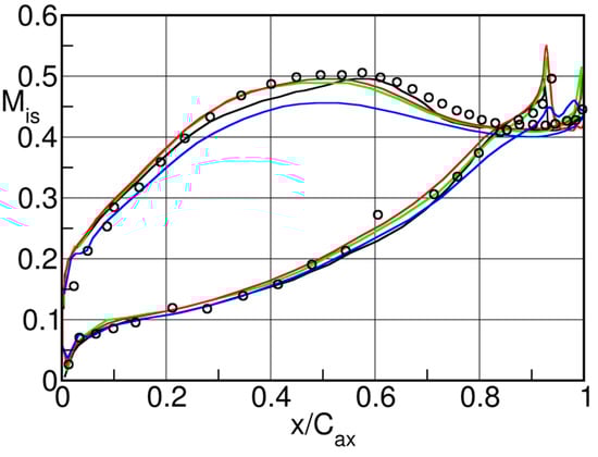
Figure 47.
VKI LS94 turbine blade, case. Time mean blade surface isentropic Mach number distribution. experiments [32];  [110];
  [111];
  [112];
  [113].
experiments [32]; [110]; [111]; [112]; [113].
The time averaged base pressure region was also fairly well reproduced by the available numerical data, although the differences among the computations and the experiments are generally larger than those reported in Figure 48. Indeed, the underlying physics is more complex, as the presence of the two pressure and suction side sharp over-expansions at the locations of the boundary layer separation suggests.
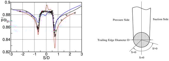
Figure 48.
VKI LS94 turbine blade, case. Time mean base pressure distribution. For symbols see Figure 47.
The location and the magnitude of these two accelerations seem within the reach of the adopted closure, as well as the pressure plateau of the base region. The predicted base pressure coefficients defined by Equation (2) agree fairly well with the experimental value, as well as with the one obtained from the VKI correlation [110]. The success of these simple models is attributed to the proper space-time resolution of the boundary layers at separation points in the trailing edge region. Again, this has been documented by Manna et al. [110] and by Sondak et al. [112] (see Figure 49) who could show a more than satisfactory agreement of the computed time averaged velocity profiles with the measured one, both on the pressure and suction sides at 1.75 diameters upstream of the trailing edge (1.75 with at the trailing edge, and ). The thinner pressure side boundary layer and the blade circulation strengthening the pressure side vortex shedding were estimated to be the cause of the higher local over expansion at the trailing edge [32]. The very consistent grid refinement study of [112] brought some improvements in the thinner and fuller pressure side boundary layers predictions. It is no surprise that with a proper characterization of the boundary layers and of the base region, the computed and measured losses agreed well.
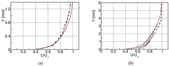
Figure 49.
VKI LS94 turbine blade, case. Time mean velocity profiles on pressure side (a) and suction side (b) at . For symbols see Figure 47.
The correct prediction of the vortex shedding frequency within experimental uncertainty proved to be more difficult, since, to this aim, the near wake physics has to be captured in terms of the large-scale coherent structures formation, development and propagation. This is probably outside the reach of any eddy viscosity closure, and most likely of the URANS approach. Also, it has been shown experimentally that the dominant frequency does not appear as a single sharp amplitude peak in the Fourier transform, but rather as a small size frequency band-width [32].
This is best seen with the help of Table 5, comparing the predicted Strouhal number with the experimental datum. Computations are assumed to report the dimensionless frequency in terms of isentropic exit velocity . The experimental Strouhal value of 0.27, has been rescaled using the nominal shedding frequency of 2.65 kHz and the isentropic velocity corresponding to the value (Cicatelli et al. [32]). Despite the use of the same simplistic closure the scatter is rather large both among the computations and with the experiments. The predicted Strouhal number of Sondak et al. [112] agrees perfectly with the experimental value.
Table 5.
VKI LS94 turbine blade, case. Strouhal numbers.
Those results obtained at a relatively low Mach number pushed the VKI group to extend the experimental investigation into the high subsonic/transonic range in 2003 [21] and 2004 [36] as already discussed in Section 3. This was a new breakthrough, as it offered once more, and again for the first time, a set of highly resolved experimental data documenting the effects of compressibility on the unsteady wake formation and development process, throwing some considerable light on the relation between the base pressure distribution and the vortex shedding phenomenon. In the next ten, fifteen years a number of research groups attempted to simulate this flow setup, mostly with higher fidelity approaches and the results were again rather satisfactory. The nominal Mach and Reynolds numbers were increased considerably ), and a variety of additional flow conditions including supersonic outlet regimes were tested, as discussed in Section 5. Table 6 summarizes the relevant contributions.
Table 6.
Available computations of the VKI LS-94 turbine blade.
For the structured meshes the number of nodes and the number of cells is similar. In the unstructured cases the difference is rather large, and typically there is a factor 5 more cells than nodes. The URANS simulations should have been carried on a two-dimensional mesh, since there is no reason for transversal modes to develop with 2D inflow conditions in a perfectly cylindrical geometry extruded by some percentage of the chord in the spanwise direction. The URANS computations of Leonard et al. [118] and those of Kopriva et al. [67] were carried out on a 3D mesh obtained expanding the 2D domain in the third direction by a fraction of the chord length (5.7% in [118] and 8% in [67]). None of the authors discussed the appearance of spanwise modes in the URANS data. Conversely, the scale resolving simulations (LES and DDES) need to be carried out on a 3D domain, with a homogeneous spanwise direction, to allow for the appropriate description of the most relevant energy carrying turbulent eddies, which are inherently three dimensional in nature. Occasionally, some authors reported two dimensional pseudo-DDES and pseudo-LES, that is, unsteady computations obtained on a purely two dimensional mesh, none of which has been included in Table 6. On the resolution side, the URANS simulations of Kopriva et al. [67] seem to have gone through some grid refinement study, while those of Leonard et al. [118] did not. On the LES and DDES side the situation is far more involved. At a Reynolds number of about three million the grid point requirements for a wall resolved LES is about [124] which is a couple of orders of magnitude higher than the most refined LES of Table 6. Thus, the very neat inertial subrange of this HPT flow is likely not to be resolved at all by any of the available simulations, and consequently the cut-off is poorly placed. These deficiencies will seriously impact on the quality of the simulations as they undermine the essential prerequisites upon which LES relies. For the DDES simulation this inconsistency is only partially relieved. Detached Eddy Simulation and similar hybrid URANS-LES approaches have somewhat met certain expectations, even though they are routinely overlooked as a means of achieving a LES-like quality at the cost of a URANS setup. Instead, DES and its evolved version DDES, should be categorized as Wall Modeled LES, and thus they can by no means be considered as a coarser grid version of LES [106]. In the present context modelling the boundary layer via URANS all the way down to the point of incipient separation will not return any of the key features the true turbulent boundary layer should possess to properly form the wake and determine its correct space time development. And relieving the Modeled Stress Depletion of DES by better addressing the URANS-LES migration in the grey area, will only partially alleviate the grid induced separation issue of these hybrid methods. All in all, the two DDES simulations of El-Gendi et al. [120,121] and Wang et al. [123] are also to be considered as unresolved, because of the previously mentioned cut-off misplacement. We shall return to this point later on.
At this high subsonic regime, the experimental time mean blade pressure distribution already presented in Figure 17 in terms of local isentropic Mach number, reveals that the flow is subsonic all around the blade.
The computations compared in Figure 50 predict fairly well the continuous acceleration of the flow both on the suction (till the throat location at 0.61) and on the pressure side (till the trailing edge). Also, the sudden deceleration from the throat to the trailing edge is well predicted by all simulations.
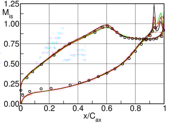
Figure 50.
VKI LS94 turbine blade, case. Time mean blade surface isentropic Mach number distribution; eddy viscosity models. experiments [21]; Baldwin & Lomax [117]; Spalart & Allmaras [117]; Wilcox - [117];  Wilcox - [118];
  Wilcox - [67].
experiments [21]; Baldwin & Lomax [117]; Spalart & Allmaras [117]; Wilcox - [117]; Wilcox - [118]; Wilcox - [67].
Leonard et al. [118] and later Kopriva et al. [67] have clearly demonstrated that a steady state solution will propose supersonic flow conditions and a normal shock on the suction side at 0.61, an artefact of the wrong modelling which disappears in the unsteady approach (see Figure 51). The trailing edge induced unsteadiness, whose upstream propagation is significant (see Figure 37), causes the shock to flap up and down on the straight rear part of the suction side, a phenomenon that causes a spatial smoothing of the pressure discontinuity at the wall and the disappearance of the supersonic pocket in a time averaged sense. In fact, it is likely that the lack of sharpness of many transonic experimentally measured surface pressure distributions obtained with slow response sensors, is to be attributed to the implicit temporal averaging resulting from the unresolved unsteadiness. Eddy viscosity and scale resolving models (Figure 52) seem to yield comparable results in a time mean sense all along the blade, while the proper prediction of the base flow appears more cumbersome. Yet, there are appreciable differences among the computations, as well as with the experiments, in the leading edge area for , whose origin is unclear. Potential sources of discrepancies are the inflow angle setting (purely axial) yielding some leading edge de-loading in the experiments, the low Mach number effects on the accuracy of compressible flow solver not relying on pre-conditioning techniques, larger relative errors of the pressure sensors in this incompressible flow region, some geometry effects. In the remaining part of the blade, trailing edge area excluded, i.e., , the agreement among all computations and experiments is very good. Surprisingly, the difficult region of the unguided turning in the rear part of the suction side () where the shock wave turbulent boundary layer interaction occurs, is well predicted in a time averaged sense by all closures.
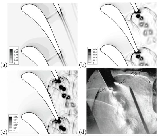
Figure 51.
VKI LS-94 turbine blade, case. Density gradient based contours; (a) RANS, -, (b) URANS, -, (c) LES, (d) Experiments, schlieren photograph. Adapted from Leonard et al. [118].
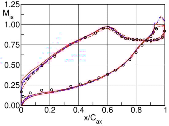
Figure 52.
VKI LS94 turbine blade, case. Time mean blade surface isentropic Mach number distribution; scale resolving simulations. experiments [21]; DDES [120, 121];  DDES [123];
  structured LES [118];
  unstructured LES [118];
  unstructured LES [56].
experiments [21]; DDES [120, 121]; DDES [123]; structured LES [118]; unstructured LES [118]; unstructured LES [56].
In the base flow region the scatter is instead remarkable, as shown in Figure 53 and Figure 54. The physics of the time averaged base pressure, consisting of three pressure minima and two maxima, has already been explained before, and will not be repeated here. What is worth mentioning is that the physical explanation offered for the disappearance of the pressure plateau at the trailing edge center at higher Mach number is thoroughly supported by the numerical results of Leonard et al. [118] and Kopriva et al. [67] (results not shown herein). In fact, when the simulations are performed with a steady-state approach there is no sudden pressure drop originated by the enrolment of the unsteady separating shear layers into a vortex right at the trailing edge, and the over-expansions occurring at the separation points are followed by a marked and unphysical recompression leading to a nearly constant pressure zone. Conversely, all unsteady simulations reproduce, at least qualitatively, the correct base pressure footprint. There is some scatter in the position of the separating shear layers as predicted by the eddy viscosity closures, a phenomenon that is related to the correct characterization of the turbulent boundary layers at the point of incipient separation. Both experiments and computations have shown in fact that there is little or no motion of the separation point along the blade surface so that the position of the over-expansion is neat both in a time averaged and instantaneous sense. Conversely, the intensity of the over-expansion strongly depends upon the pitchwise flapping motion of the shear layers, which, as shown by the experiments, is vigorous. This is necessarily smeared by the Reynolds averaging and by the time averaging. The small range of scales resolved by the eddy viscosity closures is causing the large discrepancies between the computations and the experiments.
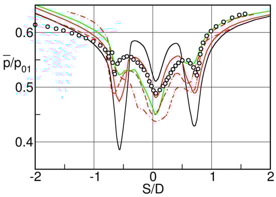
Figure 53.
VKI LS94 turbine blade, case. Time mean base pressure distribution; eddy viscosity models. For symbols see Figure 50.
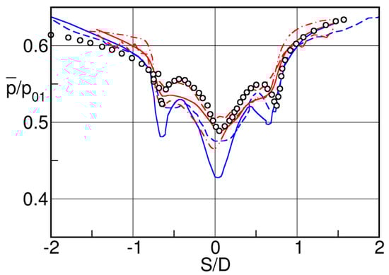
Figure 54.
VKI LS94 turbine blade, case. Time mean base pressure distribution; scale resolving simulations. For symbols see Figure 52.
Remarkably the same closure, implemented in a similar numerical technology returns very large scatters in the time averaged base pressure region (Leonard et al. [118] and Kopriva et al. [67]), a phenomenon that should be traced back to the inadequate grid resolution, both in the normal to the wall and in the streamwise direction of nearly all computations. None of the presented simulations did undergo a consistent grid refinement study in an unsteady sense, and the effects of the lack of resolution are evident from the improper prediction of the near trailing edge pressure data, that is the region at . As a matter of fact, only one out the three - contributions has an adequate first cell y+ value [67], and has attempted to investigate the effects of the grid size in an unstructured approach. The authors claimed that the coarsest grid achieved grid convergence, but, on account of the adopted technology, this conclusion is uncertain.
Scale resolving simulations presented in Figure 54, produce significant improvements in the base pressure distribution predictions, and the quality of the LES and DDES data should be considered comparable, despite the differences in modelling and grid densities, the latter playing a key role. The general trend is to under-predict the pressure level, while the shape of the wall signal, with its characteristic peak-valley structure, is well represented by all simulations. Inspection of the boundary layer profiles extracted one diameter upstream of the trailing edge circle on both sides of the blades is helpful to understand the scatter in the base pressure data. Those data are presented later on.
Before proceeding with the analysis of the boundary layers, let us briefly discuss the numerical results of Vagnoli et al. [56], whose simulations are the only one documenting the capabilities of scale resolving simulations to cope with the difficulties associated to the base flow prediction in the transonic regime, all the way up to mildly supersonic exit Mach numbers. Those data are reported in Figure 55, where some of the experimental data already presented in Figure 33 (see Section 5), are compared with the LES results obtained with the numerical setup and technology previously described. The agreement is, generally speaking, good at all Mach numbers. The shape of the static pressure traces and level of the base pressure is fairly well captured, although discrepancies exist. At and the peak-valley structure of the pressure signal with the neat pressure minimum at the center of the trailing edge is essentially reproduced, and the position of the separating shear layers is reasonable. The maximum differences appear to be in order of 10%. When the Mach number is increased to the degree of non-uniformity of the pressure distribution, quantified through the parameter (see Equation (5)) reduces drastically, ending in a pressure plateau. The disappearance of the enrollment of the shear layers into vortices in the base region characterizing the lower Mach numbers cases, and the effects of the shock patterns delaying the vortex formation downstream the trailing edge appears very well predicted, at least in a time averaged sense. Those are indeed remarkable results, still representing the state-of-the-art in the field.
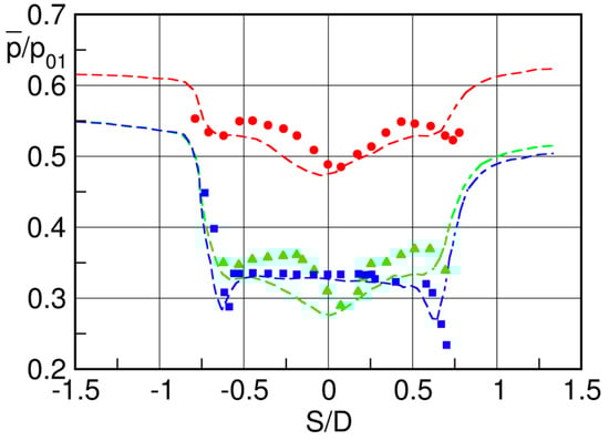
Figure 55.
VKI LS94 turbine blade. Comparison of numerical and experimental time mean base pressure distribution at transonic exit flow conditions. Symbols—experiments, lines—computations (LES). 

 . Adapted from [56].
. Adapted from [56].
Returning now to the numerical prediction of the boundary layer profiles at the trailing edge, Figure 56 shows that the eddy viscosity simulations differ considerably, both on the pressure and suction sides. Again, the two - of models of Mokulys et al. [117] and Kopriva et al. [67], disagree to some considerable extent. The results of Kopriva et al. [67] are closer to the measurements, and similar to the Baldwin and Lomax values of [117]. This last agreement seems fortuitous, and probably related to the insufficient grid resolution of Mokulys et al. [117]. The already mentioned grid refinement study of Kopriva et al. [67] is based on three unstructured grids characterized by element edge length change in the wake region of approximately 15–20%. Results presented in their study refer to near wake time averaged pressure data collected through a traverse across the wake in the direction normal to the tangent to the camber line at the trailing edge. The traverse is 2.5 trailing edge diameters downstream the trailing edge itself. Since velocity and rate of strains in the boundary layers are known to be more sensitive quantities than pressure, and on account of the convection scheme adopted in the solver, which is based on a blend of second order central differencing and first order upwinding, the achievement of grid independence with the coarsest mesh is uncertain. Yet, their - simulation is by far the best eddy viscosity result available as today. It is not a coincidence that the appropriate resolution of the boundary layers at the point of incipient separation warrants a more than satisfactory base pressure region prediction.
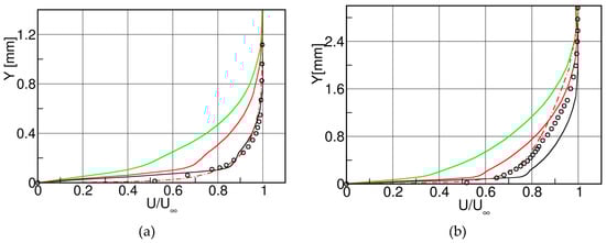
Figure 56.
VKI LS94 turbine blade, case. Time mean velocity profiles on pressure (a) and suction (b) side of the blade at . Eddy viscosity models. For symbols see Figure 50.
The scale resolving simulations here exhibit the largest differences, Figure 57. The two DDESs of El-Gendi et al. [120,121] and Wang et al. [123] predict remarkably well the suction and pressure side velocity profiles. Conversely the two LESs of Leonard et al. [118] and Vagnoli et al. [56], completely miss both profiles. There is a factor 10 in the number of grid nodes between the two DDESs and the LES of Leonard et al. [118], and a factor of 2 for that of Vagnoli et al. [56]. Furthermore, the inner layer of the LESs is either bypassed (first y+ at 5 or 40) or fully unresolved (spacing of 48 wall units along the blade height, in [56]). The major shortcoming of wall resolving LESs is precisely the inability of all subgrid scale models to reproduce the effects of the dynamics of the low speed streaks, their growth, breakdown and the wall turbulence generation process [95,102,124]. The consequence of this shortcoming is that the only successful wall resolving LESs are those whose inner layer resolution is sufficient to describe to some extent the streaks dynamics. The requirements are rather severe, since these near wall coherent structures have a typical length of 1000 wall units, a width of 30, while their average lateral spacing is in the order of 100 wall units [103,124]. They are responsible for the sweep and ejection phenomena, the inward/outward motion (with respect to the wall) of high energy fluid lumps, and therefore they are energy carrying structures. Their appropriate numerical resolution usually qualified in terms of mesh spacing in inner coordinates, is rather demanding, and also heavily depends upon the accuracy of the numerical procedure used to solve the governing equations.
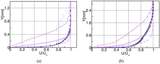
Figure 57.
VKI LS94 turbine blade, case. Time mean velocity profiles on pressure (a) and suction (b) side of the blade at . Scale resolving models. For symbols see Figure 52.
For higher order methods, viz those with spectral error decay, they can be estimated to be –, – in the streamwise and spanwise directions, respectively, while in the normal to the wall direction there should be some 10–20 points in the first 30 wall units.
These requirements are not respected by any of the two LESs clearly highlighting the inability of the SGS model to provide the correct energy contribution of the sub-grid scales to the super-grid one; it is also no surprise that the two DDESs perform better than the two LESs, thanks to the properly modelled (via -) inner wall layer. Indeed, their suction and pressure side boundary layer predictions are by far the most accurate among the available data. This is clearly shown in Figure 57. Also, the first order time integration scheme of Vagnoli et al. [56] is inadequate for a scale resolving simulation requiring a minimum time accuracy of order two. The benefit of the considerably more refined DDES meshes, allowing for the resolution of larger number of turbulent scales, should become evident elsewhere.
We next compare in Figure 58 the wake shape as predicted by the available closures. The comparison is based on a wake traverse located at 2.5 trailing edge diameters downstream the trailing edge itself, as already previously described. The prediction of a turbulent wake behind a turbine blade is a rather challenging task which is complicated by the trailing edge bluntness promoting the shedding of large-scale vortex structures. Essential for the correct prediction of the wake formation and development is the proper description of the boundary layers at the point of incipient separation. At the current Reynolds number, the scale separation is huge, and the boundary between modelled and resolved scales is uncertain, so that the extent of the grey area and the filter width may become a concern. Yet all closures seem capable to reproduce the essential features of the large-scale unsteadiness associated with the vortex shedding process; the agreement is a little more than qualitative. This is best seen in Figure 58 comparing the numerical total pressure profiles with the experimental data.
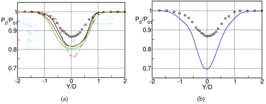
While the wake width seems fairly well predicted by all closures, the wake velocity deficit is not, by some appreciable quantities. Surprisingly, the - results of Mokulys et al. [117] look better than those of Kopriva et al. [67] despite the grid refinement study of the latter and the superior agreement in terms of boundary layer features on both sides of the blade. The DDES of El-Gendi et al. [120,121] is by far the worst of all simulations in terms of closeness to the experiments. This is surprising given the good quality of the other results extracted from the same simulation. The authors discuss in some details the potential reasons for those discrepancies, addressing numerical issues, turbulence modelling issues and grid size effects. Unfortunately, the analysis was inconclusive, and a more in-depth inspection of the data would have been necessary to identify the root reasons for the deviations documented in Figure 58. As previously detailed in this section, a DDES is characterized by three zones, namely a URANS, a LES and a hybrid one, and the extent of the latter dominates to some remarkable extent the quality of the whole simulation. The in-depth analysis of the spatial distribution of the function (see Equation (10)) (or equivalently of the in the DES-SST-zonal model) would have been of great help to identify the responsibilities of the turbulence modelling and of the filter width. What can be conjectured here, is that at the location of the wake traverses the DDES simulation is in the grey area, or, worse, in the LES one with a too large filter width. Conversely, in the base region and all around the blade in the boundary layers, the URANS mode is properly working. This can be inferred from the nearly identical boundary layer profiles as predicted by the - results of Kopriva et al. [67], and the DDES data of El-Gendi et al. [120,121], both of which qualified through an identical eddy viscosity model in the wall region (see Figure 56 and Figure 57). Thus, while the very near wake and the base region features heavily depend upon the characteristics of the boundary layers at the point of incipient separation, already a few diameters downstream the trailing edge the dynamics of the vortex shedding formation scheme is too complicate for an eddy viscosity closure as well as for an unresolved LES.
The total temperature results reported in Figure 59 are similar to the total pressure ones. All models reproduce approximately well the occurrence of the Eckert-Weiss effect, with its characteristic flow heating (respectively cooling) at the wake edges (respectively center). The magnitude of the positive and negative (compared to the inlet value) total temperature peaks, as well as their locations is only marginally well predicted by the eddy viscosity closures, while some improvements can be appreciated in the DDES of El-Gendi et al. [120,121].
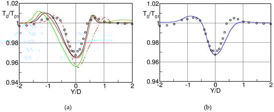
Finally, the Strouhal numbers as predicted by all numerical models are presented in Table 7.
Table 7.
VKI LS94 turbine blade, case. Strouhal numbers.
Recall that the proper evaluation of the vortex shedding frequency requires a correct modelling of the near wake mixing process, that is of the interaction between the unsteady separating shear layers [38]. The differences between the experiments and the EVM solutions are definitely larger than those pertaining to the SRS, all of which predict rather well the dominant shedding frequency. However, on account of the complexity and cost of the SRS the results obtained with the simple EVM closures are to be considered appealing. Inspection of the higher pressure modes in the near wake, both in terms of amplitude and phase, would probably underline larger differences and discrepancies.
8. Conclusions
This review manuscript has addressed in full details the flow peculiarities occurring at the trailing edge of steam and gas turbine blades, with the help of experimental and numerical data. The study is started presenting the achievements of the 40 years old VKI base pressure correlation as applied to old and new turbine blades. While the simple architecture of the formula returns satisfactorily base pressure estimates and thus loss predictions for conventional turbine blade designs, the correlation appears to fail in cases of blade designs characterized by very strong adverse pressure gradients on the rear suction side causing possibly boundary layer separation before the trailing edge. An additional weakness of the correlation resides in the fact that all experimental base pressure data are recorded by a single pressure tap in the blade trailing edges which implies the assumption of an isobaric trailing edge base pressure. This assumption is unfortunately only valid for low subsonic and supersonic Mach numbers as demonstrated recently by large scale cascade experiments.
Indeed, about twenty years after the publication of the base pressure correlation, experiments carried out at the von Kàrmàn Institute on large scale turbine blades both at subsonic and transonic outlet Mach numbers allowed major advances in the understanding of the mechanism of vortex formation and shedding in the near trailing edge wake region. Thanks to the large size of the test article, specifically designed for providing time resolved data at high spatial resolution, it has been shown that the flow approaching the trailing edge undergoes a strong acceleration both on the pressure and suction side, before leaving the blade. Two over-expansions of different strength because of the differences in the boundary layers state and of the blade circulation, have been documented and attributed to the effects of the vortex shedding. At those locations remarkable pressure fluctuations occur, reaching 80% of the outlet dynamic pressure. While at subsonic flow conditions the central trailing edge base region exhibits a rather constant pressure area, at higher Mach numbers the base pressure is characterized by the appearance of a steadily growing pressure minimum which, at the transition from a normal to an oblique trailing edge shock system, does give suddenly again way to an isobaric region. A physically consistent explanation of the departure from the assumed isobaric trailing edge base region has been proposed, and the implications with the VKI correlation outlined.
The dynamic of the shear layers has also been identified as the root cause of the formation of the acoustic wave systems occurring in the trailing edge region and their impact on the rear suction side pressure distribution.
The energy separation phenomenon, since long known to occur in cylinder flow, has been documented to also exist at the exit of transonic uncooled stator blades, causing major concerns for the mechanical integrity of the following blade row when invested by uneven total temperature distributions. Important achievements were obtained by the Canadian research group of the NRC who first measured time resolved pressure and total temperature distribution in the wake of transonic turbine blades. The data, corroborated by successive experiments, highlighted the relation between the vortex street formation and propagation with the energy separation phenomenon. High resolution experimental data were released for code-to-experiment validation and the outcome of the available simulations, presented in a dedicated section, has been discussed at length.
The turbine trailing edge frequency features, as measured on a number of blades, have been analyzed and their relations with the geometry, the boundary layer state at the point of incipient separation and the governing dimensionless parameters, clarified.
In spite of the considerable progress made so far for a better understanding of unsteady trailing edge flows and their effects on the blade performance, there is clearly room for further experimental research on unsteady trailing edge flows. The main objective should be the conception and preparation of additional large-scale cascade tests allowing high resolution spatial and temporal measurements. New benchmark test cases would then be available for experiment-to-experiment and code-to-experiment validation. The benchmark test cases presented in this paper were characterized by turbulent boundary layers on both suction and pressure sides at the point of separation from the trailing edge. It would be certainly interesting to dispose of a large-scale test case with mixed turbulent/laminar (suction side/pressure side) trailing edge flow conditions. It would also be desirable to apply high resolution fast optical measurement techniques to determine the time varying wake velocity field for the evaluation of the rate of strain and the vorticity tensors. Long time and phase averaged turbulence data will naturally come out, thus enhancing the actual knowledge of the wake mixing process. This may ultimately require the measurement of the three-dimensional time-varying velocity field. It would also be highly desirable to have more test data for the downstream evolution of the wake total temperature profile, the knowledge of which is of prime importance for the evaluation of the mechanical integrity of the downstream blade row. The reduction of the trailing edge vortex intensity and therewith the profile losses by appropriate trailing edge shaping, as e.g. elliptic trailing edges, deserves certainly further attention. Again, large scale test set up will be needed to highlight the differences in the wake mixing process.
On the numerical side the progresses achieved over 40 years of unsteady turbine wake flow computations have been impressive. This is equally due to the advances in numerical methods and modelling concepts. The authors have put together all available computations of the VKI LS94 turbine blade, whose geometry and experimental data have been previously presented. Within the bounds of the limited published material, a few concluding remarks on the ability of the adopted turbulence closures can be put forward. While the freely available turbine geometry is relatively simple, the flow conditions are not, mainly because of the large Reynolds number. Very few of the URANS contributions did achieve grid convergence in the sense of the local truncation error, in order to confine those errors at values smaller than the modelling ones. The problem of the inadequate number of numerical parameters becomes particularly offending for the scale resolving simulations (DES, DDES and LES) for which the interaction between the space-time numerical integration procedure and the turbulence closure is known to be warring, especially when implicit filtering and low order methods are used. In addition, and unlike URANS, the resolution requirements are far more stringent, and hard to satisfy.
It has been shown that the URANS calculations presently reviewed comply with the spectral gap requirement, and, therefore, the expectations of predictivity are legitimate. In fact, although a systematic grid convergence study was rarely achieved, the general quality of the numerical solutions obtained with eddy viscosity models can be rated satisfactory. Algebraic, one equation and two equations models proved capable to predict reasonably well the time averaged blade pressure distribution, even in the difficult base region, both in the subsonic and transonic regimes. Time averaged boundary layer profiles in the near trailing edge region, and even more, wake features are more problematic, especially in the high Mach number cases. Particularly, the total pressure and total temperature profiles did not go further than a qualitative agreement with the experiments, although the energy separation phenomenon was correctly represented. Scale resolving simulations improved the predictivity level of the URANS, but not as expected. Most of the deficiencies have been traced back to an inadequate sub-grid filter positioning often causing severe deviations from the experiments. The hybrid simulations were more performant than the pure LESs, mainly because of the larger number of parameters of the former. Boundary layers and even more the near wake region were poorly predicted by the scale resolving simulations, partly because of the already mentioned inertial subrange reproduction failure, a consequence of the insufficient spatial resolution, and partly because of known SGS limitations, that is their inability to provide the appropriate energy contribution of the unresolved scales to the resolved ones in regions of strong shears. The unsteady features of the flow have not been fully exploited, and thus the judgment on their quality is uncertain. The Strouhal number was reasonably well predicted by all closure.
What appears to be needed to improve the quality of the available high-fidelity TWF simulations is a more detailed and conscious selection of the spatial resolution. At high Reynolds number and even more in transonic flow conditions, this turns out to be the most difficult objective to comply with, especially because in the DES/LES world there is no equivalent of the grid convergence concept routinely applied in the URANS world to isolate the modelling errors. DES/LES have an indissoluble cut-off placement - modelling error relationship which is difficult to identify, especially when the cut-off, that is the filter width, is implicitly defined by the mesh size. In those instances, the mixture of numerical and modelling errors cannot be unraveled. Also, the presence of an inertial subrange, a pre-requisite for the correct application of the LES concept, is difficult to ascertain a-priori. Nevertheless, to acquire more credibility, the future class of numerical computations will have to provide more and more details of the resolved turbulence, presenting spectra, spatial correlations and stress tensor components of the computed fields at key locations. Those data will hopefully convince the reader of the quality of the simulations and give more confidence in the collected data. Hybrid methods will have to systematically offer quantitative details of the boundaries of the so-called grey area, to give a precise idea of what and where was modeled and resolved by the simulations. Databases of scale resolving simulations respecting certain properly defined quality criteria should be made openly available to the whole turbomachinery community for code-to-code and code-to-experiment validation.
Author Contributions
Conceptualization, methodology, formal analysis, investigation, data curation, writing—original draft preparation, writing—review and editing: C.S. and M.M. All authors have read and agreed to the published version of the manuscript.
Funding
This research received no external funding. The APC were afforded by the Dipartimento di Ingegneria Industriale of the Università degli Studi di Napoli Federico II.
Conflicts of Interest
The authors declare no conflict of interest.
List of Symbols
| Roman | Greek letters | ||
| chord | flow angles from tangential direction | ||
| skin friction coefficient | gauging angles from tangential direction | ||
| specific heat at constant pressure | trailing edge wedge angle | ||
| specific heat at constant volume | difference operator, grid spacing | ||
| base pressure coefficient | rear suction side turning angle | ||
| distance from the wall | turbulent dissipation | ||
| trailing edge thickness | momentum thickness | ||
| frequency | kinematic viscosity | ||
| pitch | turbulent viscosity | ||
| von Kàrmàn constant | vorticity, specific dissipation | ||
| thermal conductivity, | density | ||
| Mach number | stress tensor | ||
| throat, gauging angle | characteristic time | ||
| pressure | wall shear stress | ||
| pressure ratio | loss coefficient | ||
| dynamic pressure | |||
| perfect gas constant | Subscripts | ||
| Reynolds number | stagnation value | ||
| recovery coefficient | at blade inlet | ||
| specific entropy | at blade outlet | ||
| rate of strain tensor | in the axial direction | ||
| Strouhal number | boundary layer | ||
| time | at the base of the profile | ||
| temperature | at infinity | ||
| velocity components | isentropic value | ||
| friction velocity | in the normal, tangential direction | ||
| velocity magnitude | |||
References
- Traupel, W. Thermische Turbomaschinen: Erster Band Thermodynamisch-strömungstechnische Berechnung; Springer: Berlin/Heidelberg, Germany, 1977. [Google Scholar]
- Denton, J.D. Loss Mechanisms in Turbomachines. ASME J. Turbomach. 1993, 115, 621–656. [Google Scholar] [CrossRef]
- Sieverding, C.H. Base Pressure Measurements in Transonic Turbine Cascades. In Transonic Flows in Axial Turbomachines; VKI Lecture Series 84; von Karman Institute for Fluid Dynamics: Sint-Genesius-Rode, Belgium, 1976. [Google Scholar]
- Sieverding, C.H.; Stanislas, M.; Snoek, J. The Base Pressure Problem in Transonic Turbine Cascades. ASME J. Eng. Power 1980, 102, 711–718. [Google Scholar] [CrossRef]
- Graham, C.G.; Kost, F.H. Shock Boundary Layer Interactions on High Turning Transonic Turbine Cascades. In Proceedings of the ASME 1979 International Gas Turbine Conference and Exhibit and Solar Energy Conference, San Diego, CA, USA, 12–15 March 1979. ASME Paper 79-GT-37. [Google Scholar] [CrossRef]
- Sieverding, C.C.H.; Decuyper, R.; Hautot, P. Investigation of Transonic Steam Turbine Tip Sections with Various Suction Side Blade Curvatures. In Institution of Mechanical Engineers Design Conference on Steam Turbines for the 1980’s; C195/79; ImechE: London, UK, 1979. [Google Scholar]
- Craig, H.R.M.; Cox, H.J.A. Performance Estimation of Axial Turbines. Proc. Inst. Mech. Eng. 1971, 185, 407–424. [Google Scholar] [CrossRef]
- Fabry, E.; Sieverding, C.H. VKI Internal Note. unpublished. 2000. [Google Scholar]
- Martelli, F.; Boretti, A. A Simple Procedure to Compute Losses in Transonic Turbine Cascades. In Proceedings of the ASME 1985 International Gas Turbine Conference and Exhibit, Houston, TX, USA, 18–21 March 1985. ASME Paper 85-GT-21. [Google Scholar] [CrossRef]
- Granovskiy, A.; Gribin, V.; Lomakin, N. Experimental and Numerical Study of Transonic Cooled Turbine Blades. Int. J. Turbomach. Propuls. Power 2018, 3, 16. [Google Scholar] [CrossRef]
- Dvorak, R.; Safarik, P.; Vlcek, V. The Flow Past a Supersonic Trailing Edge in Transonic Turbine Cascades. Strojnicky Casopis 1978, 29, 260–269. [Google Scholar]
- Jouini, D.B.M.; Sjolander, S.A.; Moustapha, S.H. Aerodynamic Performance of a Transonic Turbine Cascade at Off-Design Conditions. ASME J. Turbomach. 2001, 123, 510–518. [Google Scholar] [CrossRef]
- Deckers, M.; Denton, J.D. The Aerodynamics of Trailing Edge Cooled Transonic Turbine Blades: Part 1—Experimental Approach. In Proceedings of the ASME 1997 International Gas Turbine and Aeroengine Congress and Exhibition, Orlando, FL, USA, 2–7 June 1997. ASME Paper 97-GT-518. [Google Scholar] [CrossRef]
- Gostelow, J.P.; Mahallati, A.; Carscallen, W.E.; Rona, A. Encounter with Vortices in a Turbine Nozzle Passage. Int. J. Rotat. Turbomach. 2012, 2012, 1–10. [Google Scholar] [CrossRef][Green Version]
- Xu, L.; Denton, J.D. The Base Pressure and Loss of a Family of Four Turbine Blades. ASME J. Turbomach. 1988, 110, 9–17. [Google Scholar] [CrossRef]
- Sieverding, C.H.; Heinemann, H. The Influence of Boundary Layer State on Vortex Shedding from Flat Plates and Turbine Cascades. ASME J. Turbomach. 1990, 112, 181–187. [Google Scholar] [CrossRef]
- Carrière, P. Analyse Theorique du Decollement et du Recollement Turbulents au Bord de Fuite d’un Aubage aux Vitesses Supersoniques. In Flow Research on Blading; Dzung, L.S., Ed.; Elsevier: New York, NY, USA, 1970. [Google Scholar]
- Sieverding, C.H.; Decuyper, M.; Colpin, J.; Amana, O. Model Tests for the Detailed Investigation of the Trailing Edge Flow in Convergent Transonic Cascades. In Proceedings of the ASME 1976 International Gas Turbine and Fluids Engineering Conference, New Orleans, LA, USA, 21–25 March 1976. ASME Paper 76-GT-30. [Google Scholar] [CrossRef]
- Jouini, D.B.M.; Sjolander, S.A.; Moustapha, S.H. Midspan Flow-Field Measurements for Two Transonic Linear Turbine Cascades at Off-Design Conditions. ASME J. Turbomach. 2002, 124, 176–186. [Google Scholar] [CrossRef]
- Corriveau, D.; Sjolander, S.A. Influence of Loading Distribution on the Performance of Transonic High-Pressure Turbine Blades. ASME J. Turbomach. 2004, 126, 288–296. [Google Scholar] [CrossRef]
- Sieverding, C.H.; Richard, H.; Desse, J.-M. Turbine Blade Trailing Edge Flows Characteristics at High Subsonic Outlet Mach Number. ASME J. Turbomach. 2003, 125, 298–309. [Google Scholar] [CrossRef]
- EL-Gendi, M.M. Effect of Trailing Edge Geometry on a Turbine Blade Base Pressure. In Proceedings of the International Symposium on Frontiers of Computational Science, Nagoya, Japan, 27–29 November 2008; pp. 197–204. [Google Scholar]
- Melzer, A.P.; Pullan, G. The Role of Vortex Shedding in the Trailing Edge Loss of Transonic Turbine Blades. ASME J. Turbomach. 2019, 141. [Google Scholar] [CrossRef]
- Lawaczeck, O.; Heinemann, H.-J. Von Kármán Vortex Street in the Wake of Subsonic and Transonic cascades. In Unsteady Aerodynamic Phenomena in Turbomachines; AGARD CP 177; AGARD: Neuilly-Sur-Seine, France, 1976. [Google Scholar]
- Heinemann, H.-J.; Bütefisch, K.A. Determination of the Vortex Shedding Frequency of Cascades with Different Trailing Edge Thicknesses. In Unsteady Aerodynamics; AGARD CP 227; AGARD: Neuilly-Sur-Seine, France, 1975. [Google Scholar]
- Han, L.S.; Cox, W.R. A Visual Study of Turbine Blade Pressure Side Boundary Layer. In Proceedings of the ASME 1982 International Gas Turbine Conference and Exhibit, London, UK, 18–22 April 1982. ASME Paper 82-GT47. [Google Scholar] [CrossRef]
- Beretta-Piccolli, F. Etude Expérimentale et Théorique D’écoulements Supersoniques au Bord de Fuite d’un Profil Isolé. Ph.D. Thesis, École polytechnique fédérale de Lausanne, Lausanne, Switzerland, 1988. [Google Scholar]
- Bölcs, A.; Sari, O. A New Base Pressure Correlation for Transonic and Supersonic Flows. In Proceedings of the ASME 1991 International Gas Turbine and Aeroengine Congress and Exposition, Orlando, FL, USA, 3–6 June 1991. ASME Paper 91-GT-324. [Google Scholar] [CrossRef]
- Hussain, A.K.M.F.; Hayakawa, M. Eduction of Large-Scale Organized Structures in a Turbulent Plane Wake. J. Fluid Mech. 1987, 180, 193–229. [Google Scholar] [CrossRef]
- Cicatelli, G.; Sieverding, C.H. A Review of the Research on Unsteady Turbine Blade Wake Characteristics. In Loss Mechanisms and Unsteady Flows in Turbomachinery; AGARD CP 571; AGARD: Neuilly-Sur-Seine, France, 1996. [Google Scholar]
- Ubaldi, M.; Zuni, P.; Campora, U.; Ghiglione, A. Detailed Velocity and Turbulence Measurements of the Profile Boundary Layer in a Large-Scale Turbine Cascade. In Proceedings of the ASME 1996 International Gas Turbine and Aeroengine Congress and Exhibition, Birmingham, UK, 10–13 June 1996. ASME Paper 96-GT-42. [Google Scholar] [CrossRef]
- Cicatelli, G.; Sieverding, C.H. The Effect of Vortex Shedding on the Unsteady Pressure Distribution Around the Trailing Edge of a Turbine Blade. ASME J. Turbomach. 1997, 119, 810–819. [Google Scholar] [CrossRef]
- Desse, J.-M. Effect of Time Varying Wake Flow Characteristics Behind Flat Plates. AIAA J. 1998, 36, 2036–2043. [Google Scholar] [CrossRef]
- Sieverding, C.H.; Cicatelli, G.; Desse, J.-M.; Meinke, M.; Zuni, P. Experimental and Numerical Investigation of the Time Varying Wakes Behind Turbine Blades. Notes Numer. Fluid Mech. 1999, 67. [Google Scholar]
- Ubaldi, M.; Zuni, P. An Experimental Study of the Unsteady Characteristics of the Turbulent Near Wake of a Turbine Blade. Exp. Therm. Fluid Sci. 2000, 23, 23–33. [Google Scholar] [CrossRef]
- Sieverding, C.H.; Ottolia, D.; Bagnera, C.; Comadoro, A.; Brouckaert, J.-F.; Desse, J.-M. Unsteady Turbine Blade Wake Characteristics. ASME J. Turbomach. 2004, 126, 551–559. [Google Scholar] [CrossRef]
- Cicatelli, G.; Sieverding, C.H.; Fevrier, N. Test Case N. 1—Turbine Blade for Time Varying Wake Flow Studies. In Numerical Methods for Flow Calculations in Turbomachines; VKI-LS 1994-06; von Karman Institute for Fluid Dynamics: Sint-Genesius-Rode, Belgium, 1994. [Google Scholar]
- Gerrard, J.H. The Mechanics of the Formation Region of Vortices Behind Bluff Bodies. J. Fluid Mech. 1966, 25, 401–413. [Google Scholar] [CrossRef]
- Carscallen, W.E.; Gostelow, J.P. Observations of Vortex Shedding in the Wake of Transonic Turbine Nozzles. In Proceedings of the V International Symposium on Transport Phenomena and Dynamics of Rotating Machinery, ISROMAC-5, Kaanapali, HI, USA, 8–11 May 1994. [Google Scholar]
- Carscallen, W.E. Private Communications. 2018. [Google Scholar]
- Sun, Y.C. The Existence of the Kàrmàn Vortex Streets of Unequal Strengths and the Possible Forms of Wake Flow Behind Bluff Bodies; Forschungsbericht; Deutsche Forschungs und Versuchsanstalt für Luft und Raumfahrt: Köln, Germany, 1983. [Google Scholar]
- Carscallen, W.E.; Oosthuizen, P.H. The Effect of Secondary Flow on the Redistribution of the Total Temperature Field Downstream of a Stationary Turbine Cascade. In Secondary Flows in Turbomachines; AGARD CP 469; AGARD: Neuilly-Sur-Seine, France, 1989. [Google Scholar]
- Carscallen, W.E.; Fleige, H.U.; Gostelow, J.P. Transonic Turbine Vane Wake Flows. In Proceedings of the ASME 1996 International Gas Turbine and Aeroengine Congress and Exhibition, Birmingham, UK, 10–13 June 1996. ASME Paper 96-GT-419. [Google Scholar] [CrossRef]
- Eckert, E.R.G.; Weise, W. Messungen der Temperaturverteilung auf der Oberfläche Schnell Angeströmter Unbeheizter Körper. Forschg. Ing. Wesen 1943, 13, 246–254. [Google Scholar] [CrossRef]
- Ryan, L.F. Experiments in Aerodynamic Coolant. Dissertations, Druckerei Leemann, Zürich, Switzerland, 1951. [Google Scholar]
- Eckert, E.R.G. Cross Transport of Energy in Fluid Streams. Wärme und Stoffübertragung 1987, 21, 73–81. [Google Scholar] [CrossRef]
- Kurosaka, M.; Gertz, J.B.; Graham, J.E.; Goodman, J.R.; Sundaram, P.; Riner, W.C.; Kuroda, H.; Hankey, W.L. Energy Separation in a Vortex Street. J. Fluid Mech. 1987, 178, 1–29. [Google Scholar] [CrossRef]
- Ng, W.F.; Chakroun, W.M.; Kurosaka, M. Time-Resolved Measurements of Total Temperature and Pressure in the Vortex Street Behind a Cylinder. Phys. Fluids 1990, 2, 971–978. [Google Scholar] [CrossRef]
- Sundaram, P.; Kurosaka, M.; Wu, J.M. Vortex Dynamics Analysis of Unsteady Wake Flows. AIAA J. 1991, 29, 321–326. [Google Scholar] [CrossRef]
- Buttsworth, D.R.; Jones, T.V. A Fast-Response Total Temperature Probe for Unsteady Compressible Flows. ASME J. Eng. Gas Turbines Power 1998, 120, 694–702. [Google Scholar] [CrossRef]
- Carscallen, W.E.; Hogg, S.I.; Gostelow, J.P.; Buttsworth, D.R. Time Resolved Measurements of the Energy Separation Process in a Transonic Turbine Vane Wake Flow. In Advanced Aerodynamics Measurement Technology (Seattle, WA, USA, 22–25 September 1997); AGARD: Neuilly-sur-Seine, France, 1998. [Google Scholar]
- Carscallen, W.E.; Currie, T.C.; Hogg, S.I.; Gostelow, J.P. Measurement and Computation of Energy Separation in the Vortical Wake Flow of a Turbine Nozzle. ASME J. Turbomach. 1999, 121, 703–708. [Google Scholar] [CrossRef]
- Gostelow, J.P.; Rona, A. Mid-span Losses in Turbine Blades at Subsonic and Supersonic Speeds. In Proceedings of the XVII International Symposium on Transport Phenomena and Dynamics in Rotating Machinery, ISROMAC-17, Maui, HI, USA, 16–21 December 2017. [Google Scholar]
- Denos, R.; Sieverding, C.H. Assessment of the Cold Wire Resistance Thermometer for High Speed Turbomachinery Applications. ASME J. Turbomach. 1997, 119, 140–148. [Google Scholar] [CrossRef]
- Mateos Prieto, J.B. Experimental Study of Unsteady Blade Trailing Edge Flow. Unpublished, VKI Project Report 2003-24. 2003. [Google Scholar]
- Vagnoli, S.; Verstraete, T.; Mateos, B.; Sieverding, C.H. Prediction of the Unsteady Turbine Trailing Edge Wake Flow Characteristics and Comparison with Experimental Data. Proc. IMechE Part A J. Power Energy 2015, 229, 487–497. [Google Scholar] [CrossRef]
- Raffel, M.; Kost, F. Investigation of aerodynamic effects of coolant ejection at the trailing edge of a turbine blade model by PIV and pressure measurements. Exp. Fluids 1998, 24, 447–461. [Google Scholar] [CrossRef]
- Heinemann, H.-J.; Lawaczeck, O.; Bütefisch, K.A. von Kármán Vortices and Their Frequency Determination in the Wakes of Profiles in the Subsonic and Transonic Regimes. In Symposium Transsonicum II; Springer: Berlin/Heidelberg, Germany, 1975; pp. 75–82. [Google Scholar] [CrossRef]
- Schlichting, H. Boundary Layer Theory, 7th ed.; McGraw Hill: New York, NY, USA, 1979. [Google Scholar]
- Sieverding, C.H. Unsteady Flow Measurements in Straight Cascades. In Symposium on Measuring Techniques in Transonic and Supersonic Cascades and Turbomachines; Bölcs, A., Fransson, T., Eds.; Juris-Verlag: Zürich, Switzerland, 1977. [Google Scholar]
- Bryanston-Cross, P.J.; Camus, J.J. Auto and Cross-Correlation Measurements in a Turbine Using a Digital Correlator. In Proceedings of the ASME 1982 International Gas Turbine Conference and Exhibit, London, UK, 18–22 April 1982. ASME Paper 82-GT-132. [Google Scholar] [CrossRef]
- Patterson, R.W.; Weingold, H.D. Experimental Investigation of a Simulated Compressor Airfoil Trailing Edge Flow Field. AIAA J. 1985, 23, 768–775. [Google Scholar] [CrossRef]
- Wissink, J.G. DNS of a separating, low Reynolds number flow in a turbine cascade with incoming wakes. Int. J. Heat Fluid Flow 2003, 24, 626–635. [Google Scholar] [CrossRef]
- Wheeler, A.P.S.; Sandberg, R.D.; Sandham, N.D.; Pichler, R.; Michelassi, V.; Laskowski, G. Direct Numerical Simulations of a High Pressure Turbine Vane. ASME J. Turbomach. 2016, 138. [Google Scholar] [CrossRef]
- Sandberg, R.D.; Michelassi, V. The current state of high-fidelity simulations for main gas path turbomachinery components and their industrial impact, Flow. Turbul. Combust. 2019, 102, 797–848. [Google Scholar] [CrossRef]
- Currie, T.C.; Carscallen, W.E. Simulation of Trailing Edge Vortex Shedding in a Transonic Turbine Cascade. ASME J. Turbomach. 1998, 120, 10–19. [Google Scholar] [CrossRef]
- Kopriva, J.E.; Laskowski, G.M.; Sheikhi, M.R. Assessment of High Pressure Cooled and Uncooled Turbine Blade Wakes via RANS and URANS at Engine Scale Conditions. In Proceedings of the ASME Turbo Expo 2013: Turbine Technical Conference and Exposition, San Antonio, TX, USA, 3–7 June 2013. ASME Paper GT2013-94285. [Google Scholar] [CrossRef]
- Thompson, J.F.; Soni, B.K.; Weatherill, N.P. Handbook of Grid Generation; CRC Press: Boca Raton, FL, USA, 1998; ISBN 9780849326875. [Google Scholar]
- Eiseman, P.R. Grid Generation for Fluid Mechanics Computations. Annu. Rev. Fluid Mech. 1985, 17, 487–522. [Google Scholar] [CrossRef]
- Wu, Z.-N.; Xu, S.-S.; Gao, B.; Zhuang, L.S. Review of Numerical Computation of Compressible Flows with Artificial Interfaces. Comput. Fluids 2007, 36, 1657–1679. [Google Scholar] [CrossRef]
- Lele, S.K. Compact Finite Difference Schemes with Spectral-Like Resolution. J. Comput. Phys. 1992, 103, 16–42. [Google Scholar] [CrossRef]
- Yee, H.C. Explicit and Implicit Multidimensional Compact High-Resolution Shock-Capturing Methods: Formulation. J. Comput. Phys. 1997, 131, 216–232. [Google Scholar] [CrossRef]
- Yee, H.C.; Sandham, N.D.; Djomehri, M.J. Low-Dissipative High-Order Shock-Capturing Methods Using Characteristic-Based Filters. J. Comput. Phys. 1999, 150, 199–238. [Google Scholar] [CrossRef]
- Canuto, C.; Hussaini, M.Y.; Quarteroni, A.; Zang, T.A. Spectral Methods in Fluid Dynamics; Springer: Berlin, Germany, 1988. [Google Scholar]
- Hesthaven, J.; Gottlieb, S.; Gottlieb, D. Spectral Methods for Time-Dependent Problems; Cambridge University Press: Cambridge, UK, 2007. [Google Scholar]
- Stewart, W.L.; Whiney, W.J.; Wong, Y. A Study of Boundary-Layer Characteristics of Turbomachine Blade Rows and Their Relation to Overall Blade Loss. ASME J. Basic Eng. 1960, 82, 588–592. [Google Scholar] [CrossRef]
- Harten, A. High Resolution Schemes for Hyperbolic Conservation Laws. J. Comput. Phys. 1983, 49, 357–393. [Google Scholar] [CrossRef]
- Shu, C.-W. TVB Uniformly High-Order Schemes for Conservation Laws. Math. Comput. 1987, 49, 105–121. [Google Scholar] [CrossRef]
- Yee, H.C. A Class of High Resolution Explicit and Implicit Shock-Capturing Methods; NASA-TM-101088; NASA Lewis Research Center: Cleveland, OH, USA, 1988. [Google Scholar]
- Harten, A.; Engquist, B.; Osher, S.; Chakravathy, S. Uniformly High Order Accurate Essentially Non-Oscillatory Schemes, III. J. Comput. Phys. 1987, 71, 231–303. [Google Scholar] [CrossRef]
- Adams, N.A.; Shariff, K. A High-Resolution Hybrid Compact E Scheme for Shock Turbulence Interaction Problems. J. Comput. Phys. 1996, 127, 27–51. [Google Scholar] [CrossRef]
- Fu, L.; Hu, X.Y.; Adams, N.A. A Family of High-Order Targeted E Schemes for Compressible Fluid Simulations. J. Comput. Phys. 2016, 305, 333–359. [Google Scholar] [CrossRef]
- Liu, X.-D.; Osher, S.; Chan, T. Weighted Essentially Non-Oscillatory Schemes. J. Comput. Phys. 1994, 115, 200–212. [Google Scholar] [CrossRef]
- Jiang, G.; Shu, C.-W. Efficient Implementation of Weighted E Schemes. J. Comput. Phys. 1996, 126, 202–228. [Google Scholar] [CrossRef]
- Pirozzoli, S. Conservative Hybrid Compact-WE Schemes for Shock-Turbulence Interaction. J. Comput. Phys. 2002, 178, 81–117. [Google Scholar] [CrossRef]
- Ghosh, D.; Baeder, J.D. Weighted Non-Linear Compact Schemes for the Direct Numerical Simulation of Compressible Turbulent Flows. J. Sci. Comput. 2014, 61, 61–89. [Google Scholar] [CrossRef]
- Zhu, J.; Shu, C.-W. A New Type of Multi-Resolution WE Schemes with Increasingly Higher Order of Accuracy. J. Comput. Phys. 2018, 375, 659–683. [Google Scholar] [CrossRef]
- Cockburn, B.; Karniadakis, G.E.; Shu, C.W. Discontinuous Galerkin Methods: Theory, Computation and Applications; Springer: Berlin/Heidelberg, Germany, 2012; ISBN 9783642640988. [Google Scholar]
- Zhou, T.; Li, Y.; Shu, C.-W. Numerical Comparison of WE Finite Volume and Runge–Kutta Discontinuous Galerkin Methods. J. Sci. Comput. 2001, 16, 145–171. [Google Scholar] [CrossRef]
- Mazaheri, A.; Shu, C.W.; Perrier, V. Bounded and compact weighted essentially nonoscillatory limiters for discontinuous Galerkin schemes: Triangular elements. J. Comput. Phys. 2019, 395, 461–488. [Google Scholar] [CrossRef]
- Chen, T.; Vasanthakumar, P.; He, L. Analysis of Unsteady Blade Row Interaction Using Nonlinear Harmonic Approach. AIAA J. Prop. Power 2001, 17, 651–658. [Google Scholar] [CrossRef]
- Chen, J.P.; Briley, W.R. A Parallel Flow Solver for Unsteady Multiple Blade Row Turbomachinery Simulations. In Proceedings of the ASME Turbo Expo 2001: Power for Land, Sea, and Air, New Orleans, LA, USA, 4–7 June 2001. ASME Paper 2001-GT-0348. [Google Scholar] [CrossRef]
- Lübcke, H.; Schmidt, S.; Rung, T.; Thiele, F. Comparison of LES and RANS in Bluff-Body Flows. J. Wind Eng. Ind. Aerod. 2001, 89, 1471–1485. [Google Scholar] [CrossRef]
- Wilcox, D.C. Reassessment of the Scale-Determining Equation for Advanced Turbulence Models. AIAA J. 1988, 26, 1299–1310. [Google Scholar] [CrossRef]
- Pope, S.B. Turbulent Flows; Cambridge University Press: Cambridge, UK, 2000; ISBN 0521591252. [Google Scholar]
- Dick, E.; Kubacki, S. Transition Models for Turbomachinery Boundary Layer Flows: A Review. Int. J. Turbomach. Propuls. Power 2017, 2, 4. [Google Scholar] [CrossRef]
- Baldwin, B.; Lomax, H. Thin-Layer Approximation and Algebraic Model for Separated Turbulent Flows. In Proceedings of the 16th Aerospace Sciences Meeting, Huntsville, AL, USA, 16–18 January 1978. [Google Scholar] [CrossRef]
- Spalart, P.R.; Allmaras, S.R. A One Equation Turbulence Model for Aerodynamic Flows. In Proceedings of the 30th Aerospace Sciences Meeting and Exhibit, Reno, NV, USA, 6–9 January 1992. [Google Scholar] [CrossRef]
- Jones, W.P.; Launder, B. The Prediction of Laminarization with a Two-Equation Model of Turbulence. Int. J. Heat Mass Tran. 1972, 15, 301–314. [Google Scholar] [CrossRef]
- Wilcox, D.C. Turbulence Modelling for CFD; DCW Industries: La Cañada Flintridge, CA, USA, 1993. [Google Scholar]
- Menter, F.R. Two-Equation Eddy-Viscosity Turbulence Models for Engineering Applications. AIAA J. 1994, 32, 1598–1605. [Google Scholar] [CrossRef]
- Rogallo, R.; Moin, P. Numerical Simulation of Turbulent Flows. Annu. Rev. Fluid Mech. 1984, 16, 99–137. [Google Scholar] [CrossRef]
- Piomelli, U.; Balaras, H. Wall-Layer Models for Large-Eddy Simulations. Annu. Rev. Fluid Mech. 2002, 34, 349–374. [Google Scholar] [CrossRef]
- Spalart, P.R.; Jou, W.-H.; Strelets, M.; Allmaras, S.R. Comments on the Feas1ibility of LES for Wings, and on a Hybrid RANS/LES Approach. In Proceedings of the First AFOSR International Conference on DNS/LES, Ruston, LA, USA, 4–8 August 1997. [Google Scholar]
- Spalart, P. Strategies for Turbulence Modelling and Simulations. Int. J. Heat Fluid Flow. 2000, 21, 252–263. [Google Scholar] [CrossRef]
- Spalart, P.R.; Deck, S.; Shur, M.L.; Squires, K.D.; Strelets, M.K.; Travin, A. A New Version of Detached-Eddy Simulation, Resistant to Ambiguous Grid Densities. Theor. Comput. Fluid Dyn. 2006, 20, 181–195. [Google Scholar] [CrossRef]
- Menter, F.R.; Kuntz, M. Adaptation of Eddy Viscosity Turbulence Models to Unsteady Separated Flow Behind Vehicles. In The Aerodynamics of Heavy Vehicles: Trucks, Buses and Trains; Lecture Notes in Applied and Computational Mechanics; McCallen, R., Browand, F., Ross, J., Eds.; Springer: Berlin/Heidelberg, Germany, 2004; Volume 19. [Google Scholar] [CrossRef]
- Manna, M.; Mulas, M. Navier-Stokes Analysis of Trailing Edge Induced Unsteady Flow in a Turbine Blade. In Numerical Methods for Flow Calculations in Turbomachines; VKI Lecture Series 1994-06; von Karman Institute for Fluid Dynamics: Sint-Genesius-Rode, Belgium, 1994. [Google Scholar]
- Mensink, C. Numerical Prediction of Periodic Vortex Shedding in Subsonic and Transonic Turbine Cascade Flows. Int. J. Numer. Meth. Fluids 1996, 22, 881–897. [Google Scholar] [CrossRef]
- Manna, M.; Mulas, M.; Cicatelli, G. Vortex Shedding Behind a Blunt Trailing Edge Turbine Blade. Int. J. Turbo Jet Engines 1997, 14, 145–157. [Google Scholar] [CrossRef]
- Arnone, A.; Pacciani, R. Numerical Prediction of Trailing Edge Wake Shedding. In Proceedings of the ASME 1997 International Gas Turbine and Aeroengine Congress and Exhibition, Orlando, FL, USA, 2–5 June 1997. [Google Scholar] [CrossRef]
- Sondak, D.L.; Dorney, D.J. Vortex Shedding in a Turbine Cascade. Int. J. Turbo Jet Engines 1999, 16, 107–126. [Google Scholar] [CrossRef]
- Ning, W.; He, L. Some Modelling Issues on Trailing Edge Vortex Shedding. AIAA J. 2001, 39, 787–793. [Google Scholar] [CrossRef]
- Deiwert, G.S.; Andrews, E.A.; Nakahashi, K. Theorethical Analysis of Aircraft Afterbody Flow. J. Spacecr. 2012, 24, 496–503. [Google Scholar] [CrossRef]
- Roberts, Q.D.H. The Trailing Edge Loss of Subsonic Turbine Blades. Ph.D. Thesis, Department of Engineering, University of Cambridge, Cambridge, UK, 1997. [Google Scholar]
- Magagnato, F.; Pritz, B.; Gabi, M. Calculation of the VKI Turbine Blade with LES and DES. Int. J. Therm. Sci. 2007, 16, 321–327. [Google Scholar] [CrossRef]
- Mokulys, T.; Congiu, F.; Rose, M.G.; Abhari, R.S. Unsteady Numerical Investigation of the Effect of Wakes with Eddy Shedding in Different Axial Turbine Aerofoils. Proc. IMechE Part A J. Power Energy 2009, 223, 1001–1016. [Google Scholar] [CrossRef]
- Lèonard, T.; Duchaine, F.; Gourdain, N.; Gicquel, Y.M. Steady/Unsteady Reynolds Averaged Navier-Stokes And Large Eddy Simulations of a Turbine Blade at High Subsonic Outlet Mach Number. J. Turbomach. 2015, 137, 4. [Google Scholar] [CrossRef]
- Smagorinsky, J. General Circulation Experiments with the Primitive Equations. Mon. Weather Rev. 1963, 91, 99–164. [Google Scholar] [CrossRef]
- EL-Gendi, M.; Doi, K.; Ibrahim, M.; Mori, K.; Nakamura, Y. Novel Flow Control Method for Vortex Shedding of Turbine Blade. Trans. Jpn. Soc. Aero. Space Sci. 2010, 53, 122–129. [Google Scholar] [CrossRef]
- EL-Gendi, M.; Doi, K.; Ibrahim, M.; Mori, K.; Nakamura, Y. Comparison Between Hot and Cold Flow Conditions of Turbine Cascades. Trans. Jpn. Soc. Aero. Space Sci. 2010, 53, 171–179. [Google Scholar] [CrossRef][Green Version]
- Nicoud, F.; Ducros, F. Subgrid-Scale Stress Modelling Based on the Square of the Velocity Gradient Tensor. Flow Turbul. Combust. 1999, 62, 183–200. [Google Scholar] [CrossRef]
- Wang, S.; Wen, F.; Zhang, S.; Zhang, S.; Zhou, X. Influence of Trailing Boundary Layer Velocity Profiles on Wake Vortex Formation in a High Subsonic Turbine Cascade. Proc. IMechE Part A J. Power Energy 2018, 233, 186–198. [Google Scholar] [CrossRef]
- Choi, H.; Moin, P. Grid-Point Requirements for Large Eddy Simulation: Chapman’s Estimates Revisited. Phys. Fluids 2012, 24. [Google Scholar] [CrossRef]
© 2020 by the authors. Licensee MDPI, Basel, Switzerland. This article is an open access article distributed under the terms and conditions of the Creative Commons Attribution (CC BY) license (http://creativecommons.org/licenses/by/4.0/).