Prediction of Crosswind Separation Velocity for Fan and Nacelle Systems Using Body Force Models: Part 1: Fan Body Force Model Generation without Detailed Stage Geometry

Abstract

Modern aircraft engines must accommodate inflow distortions entering the engines as a consequence of modifying the size, shape, and placement of the engines and/or nacelle to increase propulsive efficiency and reduce aircraft weight and drag. It is important to be able to predict the interactions between the external flow and the fan early in the design process. This is challenging due to computational cost and limited access to detailed fan/engine geometry. In this, the first part of a two part paper, we present a design process that produces a fan gas path and body force model with performance representative of modern high bypass ratio turbofan engines. The target users are those with limited experience in turbomachinery design or limited access to fan geometry. We employ quasi-1D analysis and a series of simplifying assumptions to produce a gas path and the body force model inputs. Using a body force model of the fan enables steady computational fluid dynamics simulations to capture fan–distortion interaction. The approach is verified for the NASA Stage 67 transonic fan. An example of the design process is also included; the model generated is shown to meet the desired fan stagnation pressure ratio and thrust to within 1%.

1. Introduction

In the design stage of an airframe, the external flow around all components must be considered. This is certainly important around engine nacelles, where the external flow will be affected by the operation of the fan. This interaction is dependent on both the positioning of the fan stage within the nacelle and its operating condition [1]. The state-of-the-art for engine modelling in full airframe computations is to use a simplified model of the propulsion system. This is done to reduce computational costs compared to traditional bladed Reynolds averaged Navier–Stokes (RANS) methods. These simplified models use steady computational fluid dynamics (CFD) simulations for non-uniform inflow where normally unsteady simulations would be required. They also reduce the number of grid cells needed by approximately two orders of magnitude within the turbomachinery blade rows [2].

These modelling approaches were discussed in detail in Godard et al. (2017) [3]. One of the approaches commonly employed in full airframe simulations involves using actuator disks. Actuator disks work by imposing changes to flow direction and stagnation quantities over a single plane, but are limited in their ability to reproduce the effects of the coupling between external flow and the fan. Godard et al. proposed that the main reason for this limitation comes from the fact that the actuator disk takes the inflow as is and computes the outflow accordingly, but lacks feedback effects [3]. Through-flow or body force methods are another approach that is examined to help capture this coupling effect; however, this is a higher fidelity approach and therefore requires more input information. Body force methods work by applying sources of momentum and energy in the swept volumes where the blades would normally be and were found to capture the external flow–fan coupling more accurately than actuator disks [3].

Many variations of body force methods exist; however, they usually require the user to have detailed blade geometry information available. Gong’s model [4] and its later refinements in Peters et al. (2015) [1], Hill’s model [2], as well as a lift–drag model [5] are examples of these; they require calibration based on experiments or more detailed computations, which include the blade rows in detail. This calibration therefore relies on detailed blade geometry and entails additional computational cost. Models such as those proposed by Hall et al. (2017) [6] and Pazireh and Defoe (2019) [7] have been shown to work without the need for calibration; however, they still require the blade geometry (no thickness information needed in Hall’s approach) and the gas path of the fan stage. The modelling approach of Sato et al. (2019) [8] works without the need for fan blade geometries, but still requires information on the gas path and blade leading and trailing edge meridional profiles.

Considering the usage case of an airframer assessing nacelle design early in the design phase, it is possible that the engines to be used have not yet been selected, and even if they have, it may not be possible to obtain the fan geometry and/or bypass duct gas path from the engine manufacturer. This means that the body force methods mentioned above would not be usable. Tools currently exist that allow for the creation of highly detailed stage and blade geometry; however, they generally require more experience with turbomachinery, as well as detailed information about the stage. MULTALL is an open source turbomachinery design suite that takes basic stage information and will generate 3D blades and gas paths [9]. Although simplified, these inputs still require the user to have information on the blade performance, which may be unknown, such as blade rotation speed or the stage work coefficient. The airframer is not interested in the level of fidelity of the blades or the stage; all that is required is that the body force recreates the external–internal flow interaction. Therefore, the airframer desires to create a body force model based on information that they know to some degree of accuracy, such as the required thrust, limitations on engine size, and an estimate of the fan stagnation pressure ratio (FPR) at the design point.

The objective of this paper is to introduce and assess a fan gas path and body force model generation process that enables the simulation of powered nacelles and/or full airframes without any prior detailed fan geometry information. This process consists of 1D analysis to determine the required change in flow quantities through the stage, as well as generating simplified blade camber surfaces and a gas path. The full MULTALL suite is not used since it requires too much input information for the intended level of fidelity; however, certain tools within the suite are utilized, as will be described later. A number of assumptions and simplifications are used during these steps to determine the required information. The key outcomes are that: (1) the process enables the creation of a body force model of a fan stage without a priori knowledge of detailed fan geometry or gas path; (2) this body force model, once implemented in a CFD framework, matches the design intent performance at the design point; (3) the body force model matches the desired spanwise loading at the rotor trailing edge (in this case, uniform) and yields rotor chordwise loading similar to that found in modern machines. With these outcomes met, the resulting model can also be used to assess off-design conditions.

In the first section of this paper, the body force formulation is described in detail, and its validation is demonstrated. Next, the design process is explained, and the selected camber shape is presented and shown to yield the desired loading distribution. The implementation of this process into a commercial CFD framework is discussed, and finally, an example application of the process is demonstrated.

2. Body Force Formulation

The concept of body force modelling involves replacing the physical rotor and stator blades with momentum and energy sources. These sources are added around an annulus covering the radial and axial extent of the physical blades. The sources generate the flow turning, as well as the pressure and temperature changes that occur in the real machine. These sources can be thought as a local blade force smeared across the blade pitch. The concept is visualized in Figure 1.

The momentum and energy equations are,

$$\frac{\partial \rho \overrightarrow{V}}{\partial t}+\nabla \left(\rho \overrightarrow{V}{\overrightarrow{V}}^T\right)+\nabla p-\nabla ·\tau =\rho \overrightarrow{f}$$

(1)

$$\frac{\partial \rho e_{\mathrm{t}}}{\partial t}+\nabla \left(\rho h_{\mathrm{t}}\overrightarrow{V}\right)-\nabla ·\left(\nabla ·\tau \right)=\rho \left(\overrightarrow{r}\times \overrightarrow{\omega }\right)·\overrightarrow{f}$$

(2)

where $\rho$ is the fluid density, $\overrightarrow{V}$ is the flow velocity, p is the static pressure, $e_{\mathrm{t}}$ is stagnation energy (where $\rho h_{\mathrm{t}}=\rho e_{\mathrm{t}}+p$), $h_{\mathrm{t}}$ is stagnation enthalpy, r is radius, $\omega$ is angular rotation speed, and $\tau$ is the viscous shear stress. The equations are modified to account for the momentum and energy source terms, which incorporate the effects of a body force per unit mass f.

The body force method chosen is Hall’s model [6], because it requires no calibration and therefore reduces the amount of stage information needed. The required inputs for this approach are the number of blades per row, B, the blade camber surface normal vectors, $\widehat{n}$, and the relative velocity vector, $\overrightarrow{W}$. The normal force acts to reduce the local deviation $\delta$, which is the angle between the relative velocity vector and a vector tangent to the blade camber surface in the plane shared by $\widehat{n}$ and $\overrightarrow{W}$. The source term per unit mass, here the incompressible normal force, $f_{\mathrm{n},\mathrm{i}}$, is defined as:

$$f_{\mathrm{n},\mathrm{i}}=\frac{2\pi \delta \left(\frac{1}{2}{W}^2/\left|n_{\theta }\right|\right)}{2\pi r/B}$$

(3)

The blade leading and trailing edge meridional profiles and the full machine gas path are also needed. The original Hall model was only intended to be used for low speed machines (incompressible flow), so a correction factor is added to account for compressibility since modern commercial engine fans operate at transonic relative Mach numbers. This takes the form of an added compressibility correction, K, where:

$$f_{\mathrm{n},\mathrm{c}}=K{f}_{\mathrm{n},\mathrm{i}}$$

(4)

as used in Benichou et al. (2019) [10]. This correction uses the Prandtl–Glauert rule in subsonic relative flow and the Ackeret formula in supersonic relative flow:

$$K^{\prime }=\left\{\begin{array}{cc}\frac{1}{\sqrt{1-M_{\mathrm{rel}}^2}}\hfill & M_{\mathrm{rel}}<1\hfill \\ \frac{2}{\pi \sqrt{M_{\mathrm{rel}}^2-1}}\hfill & M_{\mathrm{rel}}>1\hfill \end{array}\right.$$

(5)

and has an upper bound to avoid instabilities as the relative Mach number approaches one, giving,

$$K=\left\{\begin{array}{cc}{K}^{\prime }\hfill & K^{\prime }\le 3\hfill \\ 3\hfill & K^{\prime }>3\hfill \end{array}\right.$$

(6)

Body force models exist that have added terms to account for the blockage effects caused by the blades; this can be seen in the model used in Benichou et al. (2019) [10]. Including blockage adds complexity as it requires information on blade thickness. This was neglected in the current approach as the aim was not to generate full blade shapes and, as will be shown later, is not required to accurately predict the loading in the body force model. Simple loss models exist that require little or no calibration; however, the upstream influence of a fan on incoming flow is not significantly impacted by the viscous losses in blade rows [6] and therefore neglected in the body force model used in this paper.

3. Assessment of the Body Force Approach

A single passage bladed RANS simulation was compared against a body force model to assess the approach both with and without the compressibility correction at the design flow coefficient,

$$\varphi =\frac{V_{\mathrm{x}}}{U_{\mathrm{mid}}}$$

(7)

of 0.48, where $U_{\mathrm{mid}}$ is the rotor blade speed at midspan. The machine used was NASA Stage 67 [11]. The important features of this machine are shown in

Table 1. Important characteristics of the NASA Stage 67 rotor. Operating-point dependent values are at the design flow coefficient at 90% corrected rotational speed [11].

Parameter	Value	Parameter	Value
${\omega }_{\mathrm{corr}}$ (rad/s)	1512	B	22
$M_{\mathrm{rel},\mathrm{tip}}$	1.2	$\frac{{\overline{V_x}}^M}{U_{\mathrm{mid}}}$	0.5
FPR	1.48	${\left(\frac{r_{\mathrm{hub}}}{r_{\mathrm{tip}}}\right)}_{\mathrm{inlet}}$	0.375
${\dot{m}}_{\mathrm{corr}}$ (kg/s)	31.1	${\left(\frac{r_{\mathrm{hub}}}{r_{\mathrm{tip}}}\right)}_{\mathrm{outlet}}$	0.478
True Chord Aspect Ratio	1.56

. The overall, spanwise, and chordwise loading were examined for both the 70% and 90% speed lines.

The simulations were run using Ansys CFX 16 [12], using second order spatial discretization. The grids and computational approach were the same as those used in Hill and Defoe (2018) [2]. When the body force regions were relatively small compared to the overall size of the computational domain, it was found that decreasing the pseudo-time step from the default setting in CFX was required to obtain convergence. The bladed Stage 67 simulation used a single passage containing $3.58\times {10}^6$ cells. Two grids were used to check grid independence;

Table 2. Summary of the bladed simulations grid independence study performed by Hill and Defoe (2018) [2].

	Medium Grid	Fine Grid	Percent Change
Rotor Cell Count	$1.78\times {10}^6$	$2.45\times {10}^6$	37.6
$FPR$-1	0.493	0.496	0.71
Rotor ${\eta }_{\mathrm{is}}$	92.3%	92.3%	0

shows the results of the independence study. Less than 1% change was seen between the stagnation pressure ratio and isentropic efficiency, and it was therefore determined that the medium grid was sufficient. The simulations were steady state and used the shear-stress-transport turbulence model. The stagnation quantities were set at the inlet, and a mass flow rate boundary condition was used at the outlet. In this paper, blades with zero shear stress surfaces were used so that a direct comparison could be made against the body force model, which included only the turning (normal) force in the blade rows. The body force model consisted of a 1/16 annulus slice containing 279,760 cells. In

Table 3. Summary of the body force grid independence study preformed by Hill and Defoe (2018) [2].

	Medium Grid	Fine Grid	Percent Change
Cell Count	279,760	609,500	117%
${\overline{T}}_{\mathrm{t},2}^M/T_{\mathrm{t},1}-1$	0.130	0.130	0%

, a summary of the body force grid independence study is shown. The boundary conditions were the same as in the bladed simulations. The computational domains are shown in Figure 2. Further information on the computational setup can be found in Hill and Defoe (2018) [2].

The distributions of the work coefficient, defined as:

$$\psi =\frac{h_{\mathrm{t}}-h_{\mathrm{t},\mathrm{inlet}}}{U_{\mathrm{mid}}^2}$$

(8)

as a function of chord and along the span at the rotor trailing edge are shown in Figure 3 and Figure 4 for 70% and 90% corrected speed, respectively. The corrected speed is defined as:

$${\omega }_{\mathrm{corr}}=\frac{\omega }{\sqrt{\frac{T_{\mathrm{t},\mathrm{inlet}}}{T_{\mathrm{t},\mathrm{ref}}}}}$$

(9)

where $T_{\mathrm{t},\mathrm{ref}}=288$ K. The fraction corrected speed is ${\omega }_{\mathrm{corr}}$ normalized by the design value.

The figures include results from the Hall body force model with and without the compressibility correction, as well as the single passage results, which were circumferentially averaged. In the hub and tip regions, one would not normally expect a body force model to be particularly accurate since (at least for the simple normal force model used here) there was no consideration of the effects of secondary flows. We therefore restricted our chordwise plots to 20–80% span.

The root mean squared (RMS) difference in the local chordwise and spanwise work coefficient as a percentage of total work coefficient for the bladed simulation (mass averaged in the spanwise case) between the body force (BF) models and the bladed simulations (BS), defined as:

$$\%\mathrm{RMS}=100\times \sqrt{\frac{{\int }_0^c{\left({\psi }_{\mathrm{BS}}-{\psi }_{\mathrm{BF}}\right)}^2 dx}{c}}/{\psi }_{\mathrm{BS},\mathrm{TE}}$$

(10)

is shown in

Table 4. Work coefficient RMS errors for NASA Stage 67 at 70% corrected speed and $\varphi =0.48$.

	${\mathit{f}}_{\mathbf{n},\mathbf{i}}$ %RMS	${\mathit{f}}_{\mathbf{n},\mathbf{c}}$ %RMS	Improvement
20% Span	7.78%	6.62%	1.16%
50% Span	7.27%	2.74%	4.53%
80% Span	7.98%	3.75%	4.23%
Spanwise	4.50%	4.30%	0.20%

and

Table 5. Work coefficient RMS errors for NASA Stage 67 at 90% corrected speed and $\varphi =0.48$.

	${\mathit{f}}_{\mathbf{n},\mathbf{i}}$ %RMS	${\mathit{f}}_{\mathbf{n},\mathbf{c}}$ %RMS	Improvement
	Difference	Difference
20% Span	9.25%	5.37%	3.88%
50% Span	10.9%	1.81%	9.09%
80% Span	12.7%	2.15%	10.5%
Spanwise	8.34%	3.42%	4.92%

for the two rotational speeds for the incompressible and compressibility corrected body force approaches.

The correction factor improved the accuracy of the body force model in both the overall and chordwise loadings. The correction factor had a greater influence the larger the relative Mach number became; this was seen as the span fraction increased and as the corrected rotational speed increased. In the 70% corrected speed case, the improvement increased by approximately 3% as the span fraction increases, and in the 90% corrected speed case, this increased even further to approximately 6%. The reason for this larger improvement in the 90% corrected speed case was due to the fact that the relative Mach numbers were increased throughout the rotor. This was also seen by the fact that the improvement more than doubled throughout in this higher corrected speed case. The results showed that the body force model with a compressibility correction was capable of matching the chordwise loading to within 7%, which was deemed as an acceptable level of accuracy for this design process. The spanwise loading showed even better agreement.

4. Fan Stage Design Approach

We took the fan design point to be cruise, as this was the typical design condition for low fan pressure ratio commercial aircraft engines [13], which are of increasing interest in modern design. The benefit of selecting this typical design condition was that this is usually where the designer will have the most information about the required performance. This condition requires the specification of a cruise altitude and flight Mach number. These are quantities an airframer would normally know and provide the information needed to find inlet stagnation quantities. We employed 1D analysis to determine the flow properties through the stage to meet the desired performance at cruise. Based on the resulting flow properties, as well as a series of assumptions and geometric constraints, the gas path was defined.

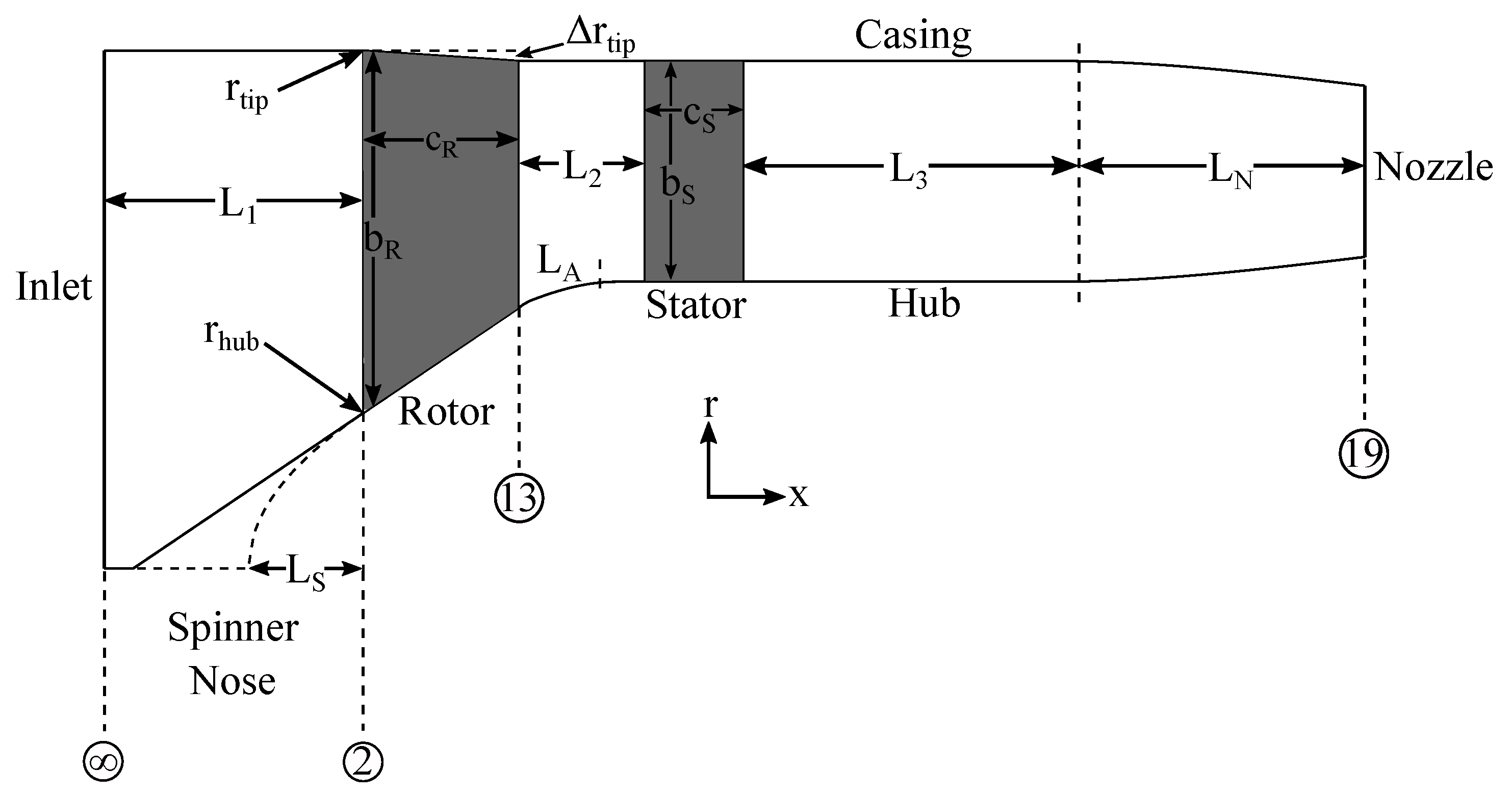
The fan pressure ratio and net thrust were required inputs. The input geometric parameters were the fan blade tip leading edge radius, rotor hub-to-tip ratio ($r_{\mathrm{hub}}/r_{\mathrm{tip}}$) at the leading edge, blade aspect ratios ($b_{\mathrm{R}}/c_{\mathrm{R}}$, $b_{\mathrm{S}}/c_{\mathrm{S}}$) based on the axial chords, axial distances upstream of, between, and downstream of the blade rows ($L_1/c_{\mathrm{R}}$, $L_2/c_{\mathrm{R}}$, $L_3/c_{\mathrm{R}}$), nozzle contraction length ($L_{\mathrm{N}}/c_{\mathrm{R}}$), hub curvature length ($L_{\mathrm{A}}/c_{\mathrm{R}}$), and fractional tip radius change through the rotor ($\Delta r_{\mathrm{tip}}/r_{\mathrm{tip}}$). A diffusion factor was specified to determine the number of rotor and stator blades, or these can be directly specified. If an elliptical spinner nose was desired, the axial length of the spinner nose, $L_{\mathrm{spin}}$, was also needed and was specified as a fraction of a linear spinner nose length. The body force model was created to generate a set fan stagnation-to-stagnation pressure ratio at a corrected mass flow, which combined with the gas path geometry, achieved the desired thrust. 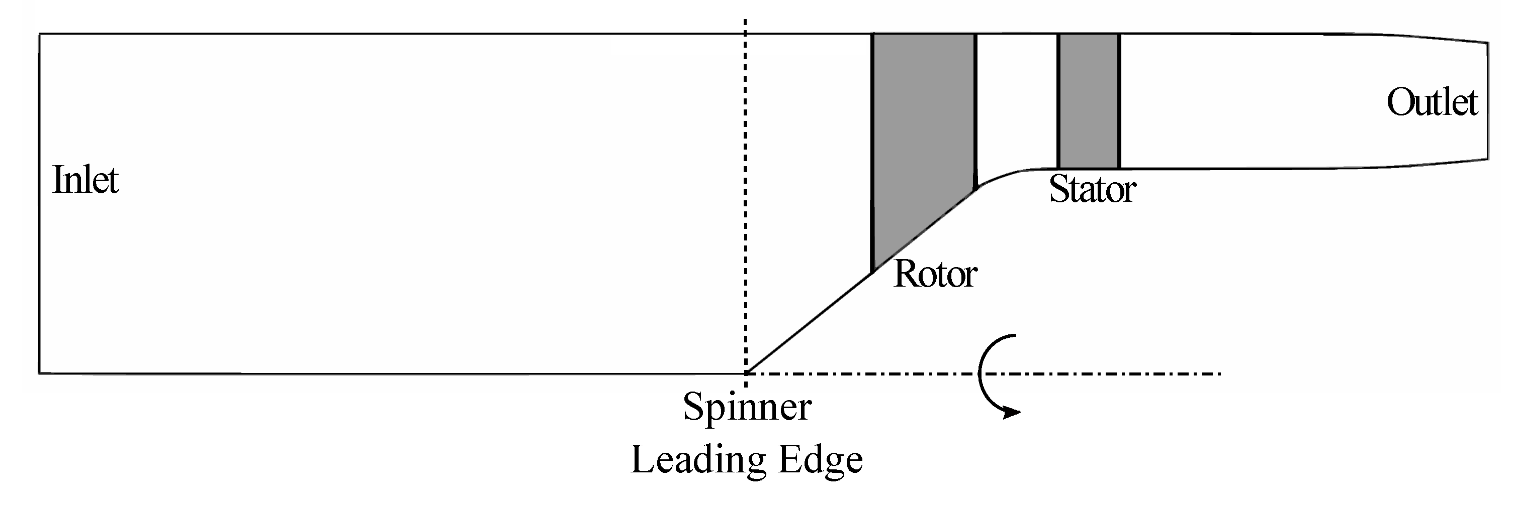Figure 5 shows the generic meridional profile of the gas path and illustrates the definitions of the geometric parameters.

The assumptions made were:

• the axial velocities at the leading and trailing edge of the blade rows were equal and constant along the span,
• the bypass ratio was high enough that the core flow contribution to thrust generation and the core suction effect on flow in the fan rotor were negligible,
• the turbomachinery and duct flow were isentropic, and
• the flow was in the meridional direction at the fan inlet.

Assumption (1) is in practice not accurate at the rapidly contracting rotor hub and would also be expected to become less accurate near the tip as the fan pressure ratio and, thus, relative Mach numbers rise. It is later shown that for the fan design space of interest, over most of the span, the variation of axial velocity was less than 10% of the assumed value. From Assumption (2), we did not include a bifurcation into a core duct in the gas path.

A simple linear scaling was used to set the blade tip relative Mach number. From the literature, it was found that modern day fans with pressure ratios of 1.6 would be expected to have a tip relative Mach number of approximately 1.4 [13,14]. We applied this scaling to set our tip relative Mach number based on the design fan pressure ratio ($FPR$):

$$M_{\mathrm{rel},\mathrm{tip}}=\frac{1.4}{1.6}FPR$$

(11)

At design, hub and casing boundary layers were thin and fully attached due to the high Reynolds numbers in practical engine fans, and thus, we assumed no changes in stagnation quantities up to the fan face; these were then set by the flight condition.

4.1. Stage Performance and Gas Path

Application of control volume analysis to the flow going through the engine yielded the standard expression for thrust:

$$F=\dot{m}(V_{19}-V_{\infty })+A_{19}\left(p_{19}-p_{\infty }\right)$$

(12)

where F is thrust, $\dot{m}$ is the mass flow rate, and A is the passage area. The thrust, flight velocity, and freestream static pressure were known at the outset, with the other quantities to be determined; this was done using a quasi-1D approach. Two cases could exist, depending on whether the exhaust nozzle was choked or not. The nozzle is choked if:

$$FPR\frac{p_{\mathrm{t},\infty }}{p_{\infty }}\ge 1.893$$

(13)

for air with specific heat ratio $\gamma =1.4$. If the nozzle is choked, the nozzle exit static pressure is:

$$p_{19}=p_{\infty }\frac{FPR}{1.893}{\left(1+\left(\frac{\gamma -1}{2}\right)M_{\infty }^2\right)}^{\frac{\gamma }{\gamma -1}}$$

(14)

If the nozzle is not choked, the nozzle exit static pressure is equal to the atmospheric static pressure:

$$p_{19}=p_{\infty }$$

(15)

The nozzle velocity, assuming isentropic flow, is:

$$V_{19}=M_{19}{\left[\gamma R\left(\frac{FP{R}^{\frac{\gamma -1}{\gamma }}{T}_{\infty }\left(1+\left(\frac{\gamma -1}{2}\right)M_{\infty }^2\right)}{1+\left(\gamma -\frac{1}{2}\right)M_{19}^2}\right)\right]}^{\frac{1}{2}}$$

(16)

If the nozzle is choked, then $M_{19}=1$, and if it is unchoked, it is determined by:

$$M_{19}={\left[{\left(\frac{p_{\mathrm{t},\infty }FPR}{p_{\infty }}\right)}^{\frac{\gamma -1}{\gamma }}-\frac{1}{\gamma -\frac{1}{2}}\right]}^{\frac{1}{2}}$$

(17)

If the flow is choked, the mass flow and nozzle area are then given by the simultaneous solution of Equation (12) and the corrected flow per unit area equation applied at Station 19,

$$\dot{m}=\frac{A_{19}{p}_{\mathrm{t},19}}{\sqrt{T_{\mathrm{t},19}}}\sqrt{\frac{\gamma }{R}}{M}_{19}{\left(1+\frac{\gamma -1}{2}{M}_{19}^2\right)}^{-\frac{\gamma +1}{2\left(\gamma -1\right)}}.$$

(18)

In Equation (18), the stagnation quantities are the mass weighted averaged values. To keep the body force model as simple as possible, we designed for uniform spanwise work input so that the local values were everywhere equal to the mass weighted averages.

If the flow was unchoked, the mass flow rate was directly calculated from Equation (12) since $p_{\infty }=p_{19}$. This along with the nozzle exit Mach number were used in Equation (18) to determine the nozzle exit area.

The axial Mach number at the fan face (Station 2) was found from Equation (18) given the fan inlet area (computed from the tip radius and hub-to-tip ratio) and the now known mass flow rate. This Mach number was then used to determine the static temperature at the fan face.

The assumption of equal leading and trailing edge axial velocities along with the selection of $FPR$ allowed the rotor trailing edge area to be calculated. In doing so, we neglected the effect of swirl on the required rotor exit area; however, within the design space typically of interest, swirl angles will normally be well under ${30}^{\circ }$, and there is only a minor effect on the required passage area [15].

The gas path shape through the rotor was generated using straight line hub and casing curves. This means that the axial velocity would vary within the blade row, but greatly simplified the generation of the gas path. A parameter, Y, which is the fraction of the fan leading edge span, set the amount of tip radius change through the rotor,

$$\Delta r_{\mathrm{tip}}=\mathrm{Y}(r_{\mathrm{tip},\mathrm{LE}}-r_{\mathrm{hub},\mathrm{LE}})$$

(19)

Downstream of the rotor, the casing radius was constant.

The slope of the hub through the rotor was set to meet the required decrease in passage area while keeping the leading and trailing edge axial velocities equal.

Downstream of the rotor trailing edge, the hub radius curved back towards axial over some desired fraction of the distance between rotor and stator ($L_{\mathrm{A}}$; the default value was $L_2/2$). The stator span was set to be constant along the chord. In reality, the removal of swirl would require a decrease in passage area, but by the same logic applied to the determination of the rotor trailing edge area, this effect is normally small.

The spinner length determined its shape. If the axial length was less than that of a straight line with the rotor hub slope extended to zero radius, then the spinner nose was assumed to be elliptical in shape. It matched the rotor hub slope downstream and extended to zero radius upstream with the tangent to the ellipse at the nose purely radial. Otherwise, a conical spinner was used with the rotor hub line extended directly down to zero radius.

4.2. Blade Performance and Camber

The rotor inlet velocity triangle at the tip, which was determined by the axial Mach number found using Equation (18) and the relative Mach number found using Equation (11), determined the rotation speed of the rotor blades.

A camber surface was needed for the body force model. Camber lines were determined at set span fractions; in the current approach, the hub, midspan, and tip were used. The camber surface was generated by fitting a 3D surface, which passed through these lines, as described in detail later in this section.

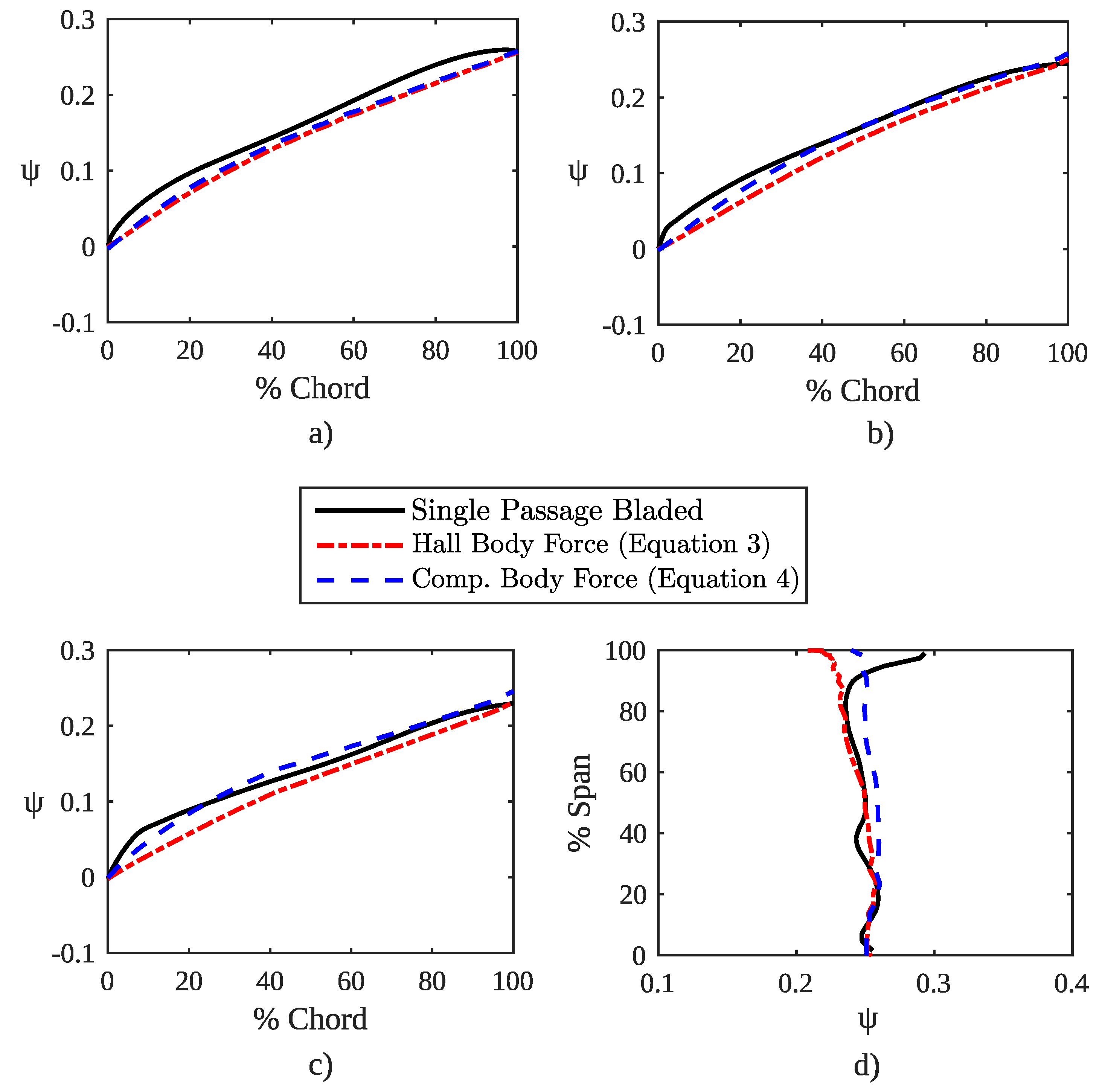
The chordwise loading distribution was shown to have an effect on inlet distortion interaction [6]; therefore, one of the aims was to generate a body force model with a camber surface that produced realistic chordwise loading distributions, while remaining relatively simple. The solution employed was to use camber shapes defined by a combination of a circular arc and a straight line. An example of this camber shape is shown in Figure 6. 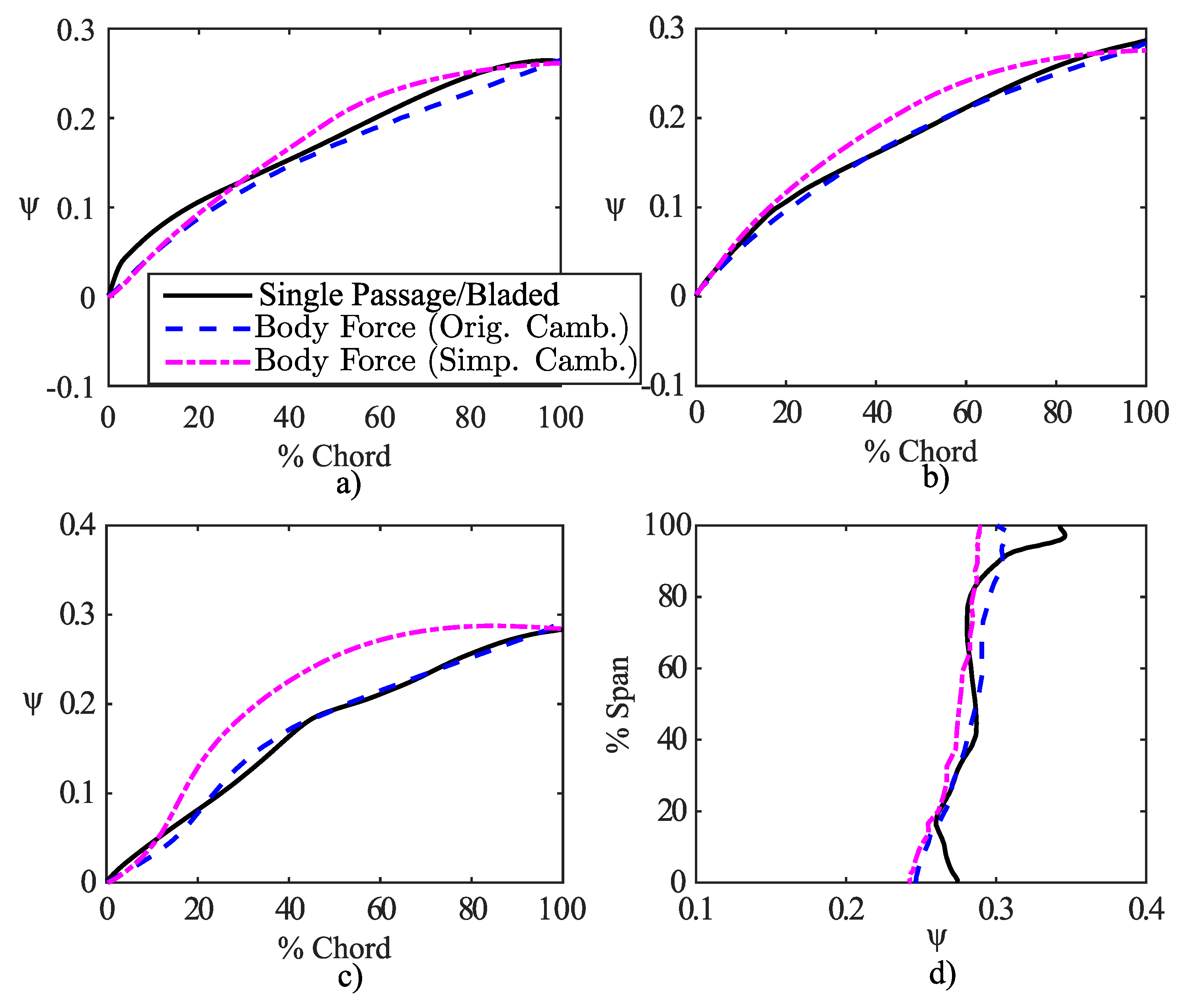In physical blades, the highest loading tends to be in the leading edge region; however, in the Hall body force model (Equation (3)), the loading scales with deviation, which tends to increase towards the trailing edge at design. The intent of pushing all camber curvature forward was to combat this effect. The straight line in the rear section of the chord worked to ensure that the required overall flow turning was met as the Hall model acted to reduce the deviation. A range of circular-straight line dividing locations was tested, and it was found that a 50:50 split between circular arc and straight line provided the best combination of guaranteeing the correct flow turning and chordwise loading distribution accuracy, as shown later. It should be noted that the model design approach did not produce realistic blade shapes, but increased the accuracy of the loading distribution of the body force model. This was a significant difference compared to the no blade information process used by Sato, Spotts, and Gao (2019) [8], as no real attempt was made to capture realistic chordwise loading in that paper.

In the design velocity triangles, the meridional velocity was used as opposed to the axial velocity. This was important because of the significant radial velocities in the rotor, especially near the hub. The consequence was that the velocity triangles and hence camber angles were dependent on the stream surface inclination since the leading and trailing edge axial velocities were assumed constant.

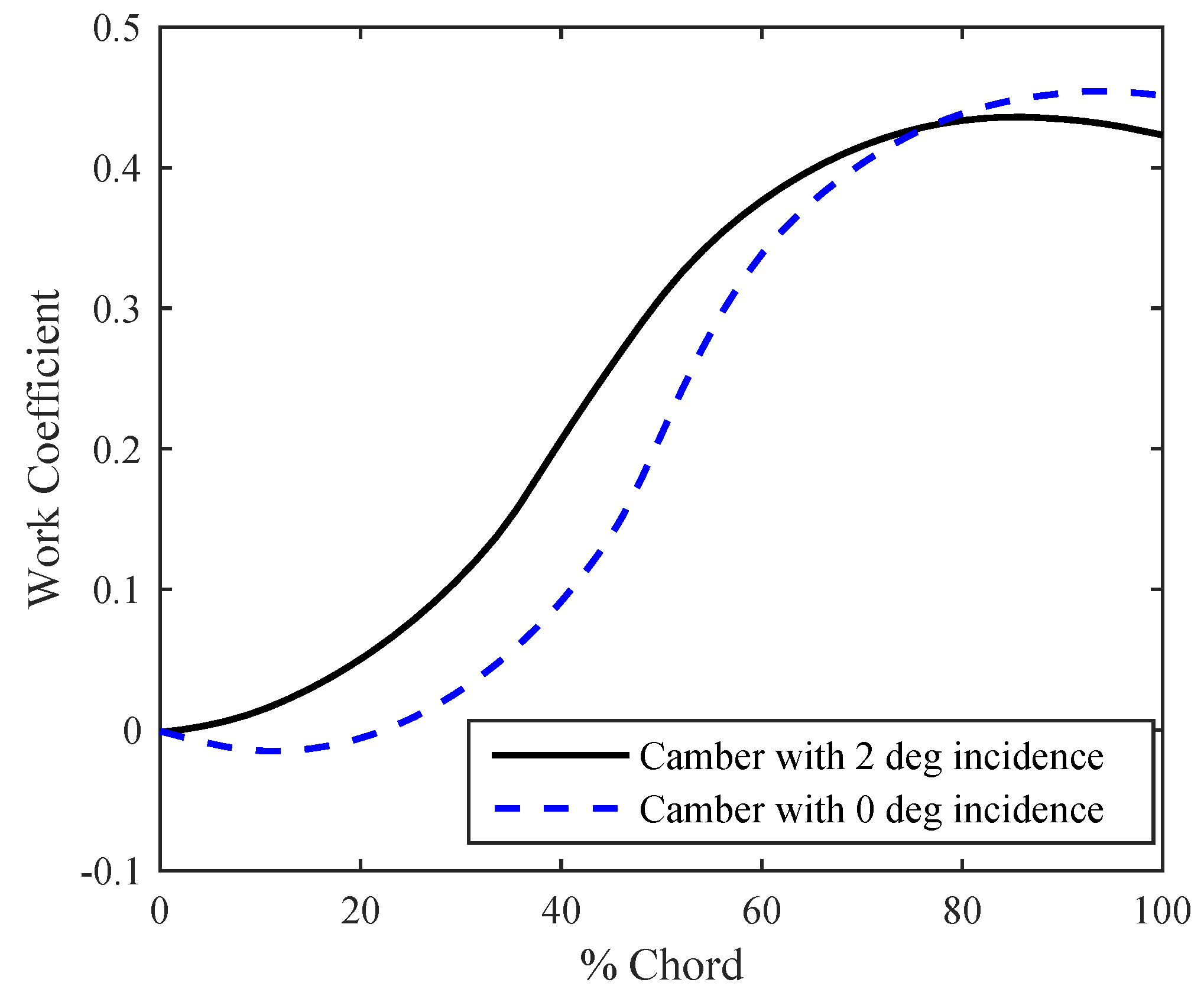
At the rotor leading edge, a small positive incidence of 2${}^{\circ }$ was used; this along with the design velocity triangles set the rotor inlet camber angle. The incidence was added to provide a more realistic chordwise loading. It increased the blade loading and flow deflection in the rotor leading edge region. This also helped ensure that the chordwise loading distributions matched predicted trends when the assumption of constant axial velocity was not realized when employing the model within a CFD simulation; if the axial velocity exceeded the assumed value, it would cause negative incidence at the leading edge, which could result in local work removal. The positive incidence acted to counteract this trend. In Figure 7, the chordwise loading is shown at 80% rotor span with and without the added incidence from the example design described later to demonstrate the difference in work addition. In the blade with 0${}^{\circ }$ incidence, the stagnation enthalpy in the first 20% chord dropped below the freestream stagnation enthalpy; this could alter the expected distortion interaction behaviour. Adding the incidence eliminated this decrease in the leading edge region. The stator leading edge camber angle was set by assuming zero incidence. Zero incidence was used for the stator leading edge because there was no change in stagnation quantities across the stator, which eliminated the need to add incidence to improve the chordwise loading distribution.

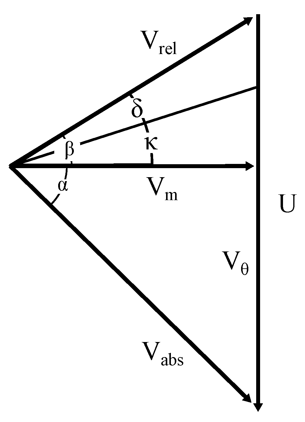
The rotor trailing edge flow angles were set based on the required work input using the Euler turbine equation,

$$c_{\mathrm{p}}(T_{\mathrm{t},\mathrm{TE}}-T_{\mathrm{t},\mathrm{LE}})=\omega (r_{\mathrm{TE}}{V}_{\theta ,\mathrm{TE}}-r_{\mathrm{LE}}{V}_{\theta ,\mathrm{LE}}),$$

(20)

the design choice to have a constant spanwise work input/pressure rise and flow deviation. The stator trailing edge was set to remove the swirl from the flow. The trailing edge angles in both blade rows accounted for the deviation. Trailing edge deviation was estimated using a modified form of Carter’s rule [13]:

$${\delta }_{\mathrm{TE}}=\left(0.23{\left(\frac{2a}{c}\right)}^2+\left(\frac{\alpha }{500}\right)\right)\xi {\left(\frac{s}{c}\right)}^{0.5}\hspace{1em}\left(\mathrm{degrees}\right).$$

(21)

where the maximum camber of the blade was at an axial distance a from the leading edge, c is the axial chord length, $\alpha$ is the exit flow angle ($\beta$ in the rotor), $\xi$ is the overall change in blade angle, and s is the pitch (spacing between blades). Carter’s rule is intended for fully circular blade camber shapes; a modification was made to a to account for the adjustment of the location of maximum camber from the mid point to the new value of 37.5% chord ($a/c=0.375$). The relationship between the flow angles ($\alpha$ and $\beta$), blade angle ($\kappa$), and deviation ($\delta$) at a rotor trailing edge are illustrated using the generic velocity triangle shown in Figure 8.

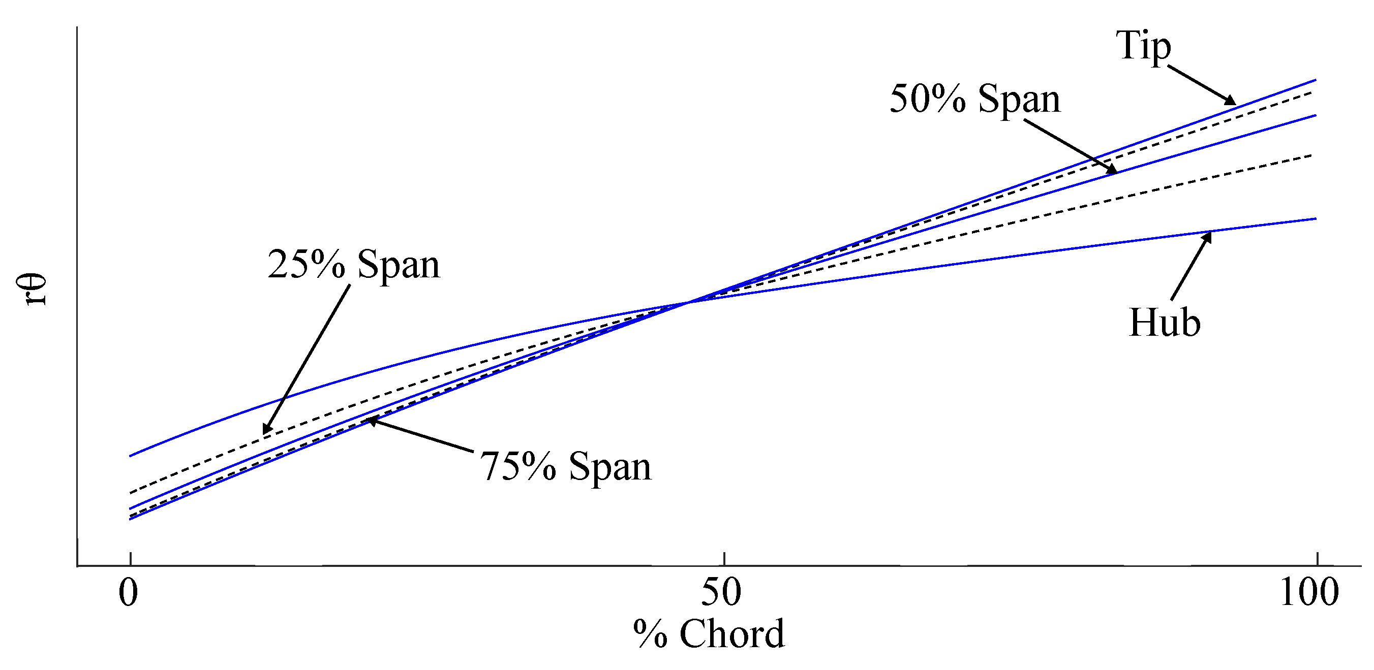
The 2D camber line sections were stacked using the open-source turbomachinery design suite MULTALL’s geometry and the grid generator Stagen. The information required for Stagen was the camber distribution and the corresponding axial and radial coordinates through the gas path at the set span fractions (0% and 100% were required; however, additional span fractions can be supplied to further constrain the design), as well as the leading and trailing edge meridional coordinates. Stagen creates a single passage grid based on the information given; the number of spanwise sections generated was equal to the number of radial grid points requested. The current maximum of 64 points was used here, which was shown to be an adequate number of radial grid points in body force models [2]. The thickness distribution was set within Stagen to produce blades of negligible thickness such that the maximum thickness was less than 1% of the blade chord. Blade thickness information was not required for the body force model, and therefore, this was done so the camber surface extraction could be simplified. The blade sections were stacked with their centroids lying along a radial line through the centroid of the hub blade section. Shown in Figure 9 are the camber lines that were produced by Stagen. The grid points on the blade surfaces were then extracted, and this was used to generate the 3D blade shapes. The camber surface was found by extracting the average of the $r\theta$ coordinates of the pressure and suction sides of the 3D blade shapes at each axial location. Finally, the camber surface normal vectors used in the compressibility corrected Hall body force model were calculated using the MATLAB [16] built-in function “surfnorm”. For more information on how Stagen works, refer to Denton (2017) [9].

5. Assessment of Camber Distribution

The ability of the half circular arc, half straight line camber shape (used in the procedure described in Section 4) to produce realistic chordwise loading distributions was assessed by using NASA Stage 67’s gas path and overall performance specifications at $\varphi =0.48$ and 90% corrected speed. Leading and trailing edge meridional profiles, as well as the gas path were kept the same as the existing NASA Stage 67 to isolate loading changes caused by camber shape. The leading edge blade angles were the same as those in the actual Stage 67 blade rows, and the rotor trailing edge blade angles for the simplified camber distribution were iteratively adjusted to minimize the %RMS error in the spanwise work coefficient distribution at the trailing edge between the simplified and original camber shapes. This ensured that the overall performance of the blade rows was similar and enabled isolation of the impact of camber shape on the loading distribution. The loading distributions are shown in Figure 10. The spanwise loading (shown in Figure 10d) $\%RMS$ difference was 3.19%; with the outer region having a larger contribution to this difference. The work coefficient in the outer region had a higher sensitivity to adjustments in blade angle, which led to increased computational costs to reduce the $\%RMS$ difference in this region; therefore, the accuracy of the trailing edge blade angle was iterated to $\pm {0.05}^{\circ }$. The chordwise loadings displayed similar overall trends, especially at lower span fractions with the $\%RMS$ difference being 6.48% and 7.43% along the 20% and 50% span lines, respectively. This slight difference was due to the modified distribution having larger work addition within the first 50% chord, but this was expected as this was where blade turning occurred. As span fraction increased, this difference became more evident as the %RMS difference increased to 13.2%; again, this stemmed from the increased sensitivity due to blade angle changes in the outer span region. The %RMS difference provided a way to compare quantitatively the loading distributions to those of a real machine; however, it was expected that the loading distributions would not be exactly the same, as the camber distributions were different. The general trends in the rate of work addition showed similarities, which was a good indication that although the camber distribution was relatively simple, it produced loadings similar to those in real machines.

6. Estimating Operating Conditions for Off-Design Thrust and Mass Flow

One of the intended uses of the models produced by the design process was to allow airframers to investigate external–fan interactions at a variety of different conditions. To investigate off-design conditions, the user must know the fraction of design inlet corrected mass flow,

$${\dot{m}}_{\mathrm{corr}}=\dot{m}\sqrt{\frac{T_{\mathrm{t}}}{T_{\mathrm{t},\mathrm{ref}}}}\left(\frac{p_{\mathrm{t},\mathrm{ref}}}{p_{\mathrm{t}}}\right)$$

(22)

as well as the flight and atmospheric conditions. Inlet corrected mass flow is a function of the fan pressure ratio and thus rotational speed. When investigating the off-design conditions, it was assumed that the fan was operating along the working line; in CFD, this required the outlet boundary condition to be set at a constant pressure. The fact that, in general, the flow coefficient is nearly constant along a fan’s working line was used to assume a linear relationship between the fraction of design inlet corrected mass flow and the fraction of design corrected speed:

$$\frac{{\dot{m}}_{\mathrm{corr}}}{{\dot{m}}_{\mathrm{corr},\mathrm{des}}}=\frac{{\omega }_{\mathrm{corr}}}{{\omega }_{\mathrm{corr},\mathrm{des}}}$$

(23)

This yielded an initial guess for the rotational speed required to drive a certain mass flow through the machine.

With the mass flow supplied, the fan inlet axial Mach number can be found using Equation (18) at the fan face, and subsequently, the static temperature can be found. With the axial Mach number and static temperature, the axial velocity was known. It was again assumed that the axial velocity was equal at the rotor leading and trailing edges. While this assumption was acceptable for the design condition, it would be far less accurate off-design; however, this was only used as an initial estimate, which was then later corrected through an iterative process. Using the new velocity triangles and the blade angles set at design, the Euler turbine equation, Equation (20), was used to determine the rotor outlet stagnation temperature, and this was then used to determine the rotor outlet stagnation pressure. The stagnation quantities were found at the hub, 50% span, and the casing; a parabolic curve was then fit to these points, and that was used to mass average analytically the rotor outlet stagnation conditions. Using the stagnation quantities at the rotor outlet, the same steps as before were used to determine the axial velocity, static temperature, and static pressure at the nozzle exit. With the static pressure and temperature known, the density at the nozzle exit was found, which allowed for the mass flow rate to be computed. This mass flow rate was compared to the desired mass flow rate, and the process was repeated with the rotational speed altered until the desired mass flow rate was achieved. This provided an initial guess for the rotational speed; however, CFD simulations must be run and the rotational speed adjusted to verify that the off-design operating point has been correctly found. An example of this process is shown later in this paper, and the off-design predictions were compared to those found using CFD; the overall 1D performance prediction matched to within 2%.

7. Implementation of the Body Force Model Generation Approach

The design process was implemented as a MATLAB [16] code, but could be implemented in any scientific computing system. It generated the hub and casing curves, as well as the 2D blade camber lines at the hub, 50%, and tip span fractions. The blade camber surface extraction process was also done within MATLAB. The process ran on a personal workstation and was computationally inexpensive. Computational run times for all steps (including Stagen) were typically under two minutes.

8. Implementation in 3D CFD

Hub and casing curves, as well as the the blade leading and trailing edge profiles were imported into grid generation software (here, Pointwise v18 [17]) to generate the gas path and demarcate blade swept volumes, which must be designated as separate cell zones.

Shown in Figure 11 is a computational domain created using this process. The upstream and downstream boundaries were placed 1.2 and one fan diameters from the rotor leading edge, respectively. These were set far enough away to provide clean inflow and avoid possible interactions with the blade rows. The process created a constant radius (equal to blade tip radius) casing curve upstream of the rotor blades. It should also be noted that in the CFD grid, the outlet nozzle was manually cut slightly before the throat area ($A^{*}$); in the example case, this was at $A/A^{*}=1.08$ (nozzle length cut by 10% before the throat area). This was done to avoid having a Mach number equal to one occurring at a boundary condition, which was found to lead to stability issues in some solvers.

Four grid levels were used to assess grid independence. A five degree slice of the full machine was used with uniform inflow. This saved computational cost as the body force model produced circumferentially uniform flow when the inflow was uniform. Simulations were run at the design operating point for the design detailed in the next section. All grids were fully structured using hexahedral cells with higher mesh density in the bladed areas. A summary of the grids tested is in

Table 6. Summary of the grid independence study for the example design in the next section.

Overall Cell Count	(x, r, $\mathit{\theta }$) Grid Count	Percent Change in
		Pressure Rise Coefficient
30,024	(147, 25, 10)	N/A
123,480	(288, 50, 10)	8.1%
464,310	(474, 100, 11)	1.5%
914,860	(621, 150, 11)	0.9%

. Only a 0.9% change in pressure rise coefficient was seen from the second finest grid to the finest grid, and therefore, the second finest grid was chosen as the final grid level.

The computations were carried out using Ansys CFX v18.2 [12], using the same boundary condition types described in the NASA Stage 67 body force simulations at the design operating point; however, at off-design operating points, the outlet static pressure was fixed based on the atmospheric conditions being tested, and the rotational speed was adjusted until the desired mass flow was reached. This was done to remain on the fan working line. The hub and casing were set as zero shear stress walls as the model assumed no losses.

9. Example Application of the Process

In this section, we present an example application of the model generation process and its implementation into CFD. The main purpose of this example was to show the level of expected accuracy of the desired performance at design and therefore assumed that there was no inlet distortion or separation. In Part 2 of this paper [18], the ability to predict these flow phenomena is examined. The example design discussed was based a on high bypass ratio turbofan engine for a medium range jet airliner. Where possible, the parameter values were based on publicly available information for the Pratt & Whitney 1524G engine and the Airbus A220-300 (formerly Bombardier CS300) aircraft. The cruise $FPR$ for the 1524G was estimated to be 1.4 [14]. This and other key design parameters that were used in this example are shown in

Table 7. Key design parameters.

Parameter	Value	Parameter	Value
$FPR$	1.4	$b_{\mathrm{R}}/c_{\mathrm{R}}$	2.33 [20]
Thrust at cruise	16.75 kN	$b_{\mathrm{S}}/c_{\mathrm{S}}$	2.25 [20]
Fan tip diameter	1.85 m [21]	$L_1/c_{\mathrm{S}}$	8.00
Fan hub-to-tip ratio	0.3 [20]	$L_2/c_{\mathrm{S}}$	0.813 [20]
Cruise Mach number	0.78 [22]	$L_3/c_{\mathrm{S}}$	2.00
Cruise altitude	10,668 m [14]	$L_{\mathrm{N}}/c_{\mathrm{S}}$	2.00

. Data sources for most specific values are cited within the table. Static thrust at sea level is 103 kN [19]. As described in Cumpsty and Heyes [14], for a high bypass ratio, low fan pressure ratio engines, typically, the ratio between sea level static and cruise thrust is between six and 6.5; in this paper, we used a ratio of 6.15. The aspect ratios were based on midspan chord values. $L_1$ was chosen to ensure the imposition of flow direction at the computational inlet boundary did not directly affect the flow within the rotor, as discussed in the previous section. $L_2$ was based on the distance between the rotor at the stator at the hub for the 1524G engine. $L_3+L_{\mathrm{N}}$ was set as discussed in the previous section and was evenly divided between the two parameters.

In this example application, the number of rotor and stator blades was supplied based on best estimates for the Pratt & Whitney 1524G engine and were 18 and 36, respectively [20]. The spinner nose was set such that the rotor hub slope line was extended to zero radius.

9.1. Results at the Design Point

These inputs produced a stage with the gas path shown in Figure 11. The rotational speed of the rotor (camber lines shown in Figure 9) was 374 rad/s, and the required mass flow was 182 kg/s. The computed increase in the mass averaged fan stagnation pressure ratio across the rotor ($FPR$-1) was found to be 0.395, which was 1.25% below the design intent, and the mass averaged stage work coefficient was found to be 1.9% lower than the desired value. Using the mass averaged Mach number at the outlet boundary, it was found that the area that would create choked flow was 0.8% lower than that generated by the design code. This resulting smaller area required was a result of the stage slightly under-predicting the $FPR$ and work coefficient. If the flow was to be isentropically brought to the nozzle area for choke, the thrust generated would be 0.14% lower than the desired thrust. In Figure 12, the rotor chordwise and trailing edge spanwise work coefficients are shown. The spanwise trailing edge work distribution had an RMS difference of 0.6% from the mass averaged overall work coefficient, so the goal of uniform outlet stagnation temperature was largely achieved.

The loading was compared against a 1D prediction generated using the Euler turbine equation, which assumed constant axial velocity through the blade row, as well as a linear build-up of deviation along the chord. The 1D prediction had a discontinuity of slope at the transition from circular arc to straight line camber. The chordwise loading was well predicted at lower span fractions with %RMS differences between the 1D prediction and the CFD being 4.12% and 4.09% at the 20% and 50% span fractions, respectively; however, as the span fraction increased to 80% span, the accuracy decreased, and the %RMS difference increased to 14.5%. The error in the prediction stemmed from the difference in axial velocity between the 1D prediction and the CFD simulations. The assumption of equal axial velocity at the blade leading and trailing edge and along the span was not borne out upon model implementation, in part due to the redistribution of the transonic relative flow. In Figure 13, the chordwise flow coefficients at set spans within the rotor are compared; equal axial velocities at the leading and trailing edge would result in all the lines starting and ending at a value of 0.64.

The flow coefficient and the local work input were inversely related to one another for a given rotational speed. This trend matched what was displayed at the leading and trailing edge regions in the chordwise loading distributions shown in Figure 12. This further confirmed the need for positive incidence at the rotor leading edge, as this variation in velocities caused a change in inlet relative flow angle. This was the result of the lack of consideration of 2D/3D effects in the design process.

The largest difference in flow coefficient was found to be a deficit of 0.22 in the rotor hub leading edge region, which corresponded to an increase in the relative flow angle of 11${}^{\circ }$. This rather large difference in relative flow angle had minimal impact on the local work coefficient when compared to the predicted value, as shown in Figure 12a. This change had a minor impact on the overall work input because it occurred at a low span fraction, and also, the hub leading edge blade angle was relatively small.

The goal was to create a chordwise loading distribution similar to those seen in modern machines. This is a qualitative goal, as there is no one correct solution. The lower 80% span fractions seemed to be producing acceptable chordwise loading distributions as work was increasing almost linearly along the chord, similar to what was seen in Stage 67. However, in the upper 20% span, the work coefficient increased to a maximum and then slightly decreased through the last 10–15% chord. This behaviour was caused by a combination of two effects. The first was the variation in spanwise axial velocity mentioned prior, and the second was the deviation buildup along the chord. Shown in Figure 14 is the deviation through the rotor at the tip. The local flow coefficient trend at the tip was similar to that shown in Figure 13 at 80% span, so we used the 80% span curve from Figure 13 and the deviation behaviour shown in Figure 14 to explain the work addition trend from Figure 12c. In the prediction code, the deviation linearly changed from the 2${}^{\circ }$ caused by the incidence to the final predicted value. In the body force simulation, the deviation was initially higher than assumed, but the body force always acted to reduce deviation; this occurred over the first 10% chord. The deviation then rose through a combination of two effects: the flow coefficient decreased (see Figure 13), and the camber surface turned away from the relative flow direction over the first 50% chord. Thus, the slower flow was unable to turn fast enough, and the deviation rose. At 50% chord, the camber shape became straight, and the body force caused the relative flow to move towards the camber surface direction, decreasing the deviation. From 50% to 80% chord, the flow coefficient was less than the design intent value, so the deviation dropped rapidly. At 80% chord, the flow coefficient rose again to be higher than the design intent value. Since when deviation was zero (near 80% chord), the body force was also zero, there was little change in tangential velocity. The increase in axial velocity associated with a rising flow coefficient means that the relative flow angle decreased, in this case to less than the camber angle, and the deviation became negative. Between 80% chord and the trailing edge, the body force acted to turn the flow back towards the camber surface, leading to work removal. The buildup of deviation was not known a priori and therefore made it difficult to predict the severity of this work removal. The overall work addition was very well predicted and showed that keeping the rear 50% camber angle constant worked as intended to ensure the correct work addition by the rotor trailing edge.

9.2. Results Off-Design

The off-design point of interest in this example was the start of take-off roll condition, with no forward movement of the aircraft. The desired corrected mass flow at take-off was chosen to be 114% of the design; the initial prediction for corrected rotation speed was found to be 119%. After running detailed CFD, it was found to be 116%. The thrust was lower than the thrust found by the 1D mass averaged take-off prediction code by 1.79%, which stemmed from the CFD producing an FPR of 0.016 less than the 1D prediction.

In Figure 15, the trailing edge work coefficient is shown, and as can be seen, the prediction code did not accurately capture the spanwise loading correctly. This inaccuracy was not unexpected as running at off-design conditions modified the velocity triangles to an extent that the simplifying assumptions within the prediction code were no longer valid. A large decrease in the meridional velocity at the tip caused by a large increase in density, which was not captured within the prediction code due to the simplifying assumptions, was the cause of the increased work coefficient.

The prediction code struggled at reproducing the chordwise and spanwise distributions off-design due to the simplifying assumptions; however, it was still beneficial since its estimated overall off-design performance and angular velocity were accurate to within 2% and 3%, respectively. This saved computational time by reducing the amount of iterations required in the CFD.

10. Summary and Conclusions

In this paper, a process was described that generated a fan gas path and body force model that met the performance requirements specified. This process differed from existing approaches in that it did not require information about blade or gas path geometry. The body force model used Hall’s formulation with an added compressibility correction. This approach was assessed by comparing the results to those found with traditional single passage simulations using the NASA Stage 67 fan geometry. Good agreement was seen with the max %RMS difference in the chordwise and spanwise work coefficient being 6.62% and 4.40%, respectively.

CFD simulations using the models produced matched the desired performance well at the design point, where the desired fan stagnation pressure ratio and thrust agreed to within 1.25%. The design objective of constant spanwise work addition was met as the RMS variation was 0.6% from the mass averaged overall work coefficient. The simplified camber distribution was used with NASA Stage 67 information to assess if the chordwise loading produced was realistic. The chordwise loading within the inner 80% span matched closely to those produced by the NASA Stage 67 with the %RMS being below 8%, with the remaining outer span showing reduced agreement with a %RMS of 13.2%. The agreement in the outer span could be improved by adjusting the ratio between the circular arc and straight line camber distribution; in this case, increasing the fraction of chord, which was a circular arc section, would create a loading distribution more similar to that of the NASA Stage 67. This suggests that the camber distribution could be a function of span, but there is no a priori way to know how one should do this; this is the reason we retained the constant 50:50 split in this paper. The rates of work addition through the rotor showed similarities, which indicates that the simplified camber distributions were producing realistic loading distributions when considering the intended use and level of fidelity. The intended use of this process was not for fan design, but for assessing external flow–fan interactions when limited fan information is available. This process created the fan stage gas path and body force model, which would be integrated into a nacelle and run in full wheel simulations. This is useful when airframers wish to investigate coupling between non-uniform inflows caused by off-design operation and the engine fan, such as a take-off with crosswind. That is precisely the focus of Part 2 of this paper [18], where we show that a fan model developed according to the procedure described in the current paper predicts crosswind separation velocity to within 5% of the value found when a detailed fan body force model is employed.

References

1. Peters, A.; Spakovszky, Z.S.; Lord, W.K.; Rose, B. Ultrashort Nacelles for Low Fan Pressure Ratio Propulsors. J. Turbomach. 2015, 137, 021001. [Google Scholar] [CrossRef] [Green Version]
2. Hill, D.; Defoe, J. Innovations in Body Force Modeling of Transonic Compressor Blade Rows. Int. J. Rotat. Mach. 2018, 2018, 6398501. [Google Scholar] [CrossRef]
3. Godard, B.; Jaeghere, E.; Nasr, N.; Marty, J.; Barrier, R.; Gourdain, N. Methodologies for Turbofan Inlet Aerodynamics Prediction. In Proceedings of the 35th AIAA Applied Aerodynamics Conference, Denver, CO, USA, 5–9 June 2017; AIAA: Reston, VA, USA, 2017. [Google Scholar] [CrossRef]
4. Gong, Y.; Tan, C.S.; Gordon, K.A.; Greitzer, E.M. A Computational Model for Short-Wavelength Stall Inception and Development in Multistage Compressors. J. Turbomach. 1999, 121, 726–734. [Google Scholar] [CrossRef]
5. Thollet, W.; Dufour, G.; Carbonneau, X. Assessment of Body Force Methodologies for the Analysis of Intake-Fan Aerodynamic Interactions. In Proceedings of the ASME Turbo Expo 2016, Seoul, Korea, 13–1 June 2016; ASME: New York, NY, USA, 2016. [Google Scholar] [CrossRef]
6. Hall, D.; Greitzer, E.; Tan, C. Analysis of Fan Stage Conceptual Design Attributes for Boundary Layer Ingestion. J. Turbomach. 2017, 139, 071012. [Google Scholar] [CrossRef] [Green Version]
7. Pazireh, S.; Defoe, J. A No-Calibration Approach to Modeling Compressor Blade Rows with Body Forces Employing Artificial Neural Networks. In Proceedings of the ASME Turbo Expo 2019, Phoenix, AZ, USA, 17–21 June 2019; ASME: New York, NY, USA, 2019. [Google Scholar] [CrossRef]
8. Sato, S.; Spotts, N.; Gao, X. Validation of Fan Source Term Model Constructed without Blade Geometry. In Proceedings of the AIAA Scitech 2019 Forum, San Diego, CA, USA, 7–11 January 2019; AIAA: Reston, VA, USA, 2019. [Google Scholar] [CrossRef]
9. Denton, J. Multall—An Open Source, Computational Fluid Dynamics Based, Turbomachinery Design System. J. Turbomach. 2017, 139, 121001. [Google Scholar] [CrossRef]
10. Benichou, E.; Dufour, G.; Bousquet, Y.; Binder, N.; Ortolan, A.; Carbonneau, X. Body Force Modelling of the Aerodynamics of a Low-Speed Fan Under Distorted Inflow. Int. J. Turbomach. Propuls. Power 2019, 4, 29. [Google Scholar] [CrossRef] [Green Version]
11. Strazisar, A.; Wood, J.; Hathaway, M.D.; Suder, K. Laser Anemometer Measurements in a Transonic Axial-Flow Fan Rotor; Techreport 2879; NASA: Washington, DC, USA, 1989.
12. ANSYS Inc. ANSYS v18.2 User’s Guide; ANSYS Inc.: Canonsburg, PA, USA, 2017. [Google Scholar]
13. Dixon, S.; Hall, C. Fluid Mechanics and Thermodynamics of Turbomachinery, 7th ed.; Butterworth-Heinemann: Oxford, UK, 2014. [Google Scholar] [CrossRef]
14. Cumpsty, N.; Heyes, A. Jet Propulsion, 3rd ed.; Cambridge University Press: Cambridge, UK, 2015. [Google Scholar] [CrossRef]
15. Greitzer, E.M.; Tan, C.; Graf, M.B. Internal Flow, 1st ed.; Cambridge University Press: Cambridge, UK, 2004. [Google Scholar] [CrossRef]
16. Mathworks Inc. MathWorks MATLAB 2017 Documentation; Mathworks Inc.: Natick, MA, USA, 2017. [Google Scholar]
17. Pointwise. Pointwise v18.0R4 User’s Manual; Pointwise: Forth Worth, TX, USA, 2017. [Google Scholar]
18. Minaker, Q.J.; Defoe, J.J. Prediction of Crosswind Separation Velocity for Fan and Nacelle Systems Using Body Force Models: Part 2: Comparison of Crosswind Separation Velocity with and without Detailed Fan Stage Geometry. Int. J. Turbomach. Propuls. Power 2019, 4, 41. [Google Scholar] [CrossRef] [Green Version]
19. EASA. TYPE-CERTIFICATE DATA SHEET No. IM.E.090 for PW1500G Series Engines; Techreport; European Union Aviation Safety Agency: Cologne, Germany, 2019.
20. Transportation Safety Board of Canada. Aviation Investigatation Report A14Q0068; Techreport; Government of Canada: Gatineau, QC, Canada, 2016.
21. Pratt and Whitney. PW1500G, AIRBUS A220 PRODUCT CARD. Available online: http://newsroom.pw.utc.com/download/PW1500G.pdf (accessed on 13 December 2019).
22. Bombardier. C Series. Available online: http://commercialaircraft.bombardier.com:80/content/dam/Websites/bca/literature/cseries/Bombardier-Commercial-Aircraft-CSeries-Brochure-en.pdf.pdf (accessed on 8 September 2015).
Figure 1. Comparison of the physical blades (left) and the source term model (right).
Ijtpp 04 00043 g001
Figure 2. Computational domains of (a) the single passage bladed RANS simulations and (b) the body force simulations.
Ijtpp 04 00043 g002
Figure 3. Work coefficient vs. meridional distance through the rotor at: (a) 20% span, (b) 50% span, (c) 80% span, and (d) rotor trailing edge at 70% corrected speed and ϕ = 0.48 .
Ijtpp 04 00043 g003
Figure 4. Work coefficient vs. meridional distance through the rotor at: (a) 20% span, (b) 50% span, (c) 80% span, and (d) rotor trailing edge at 90% corrected speed and ϕ = 0.48 .
Ijtpp 04 00043 g004
Figure 5. Meridional profile displaying the geometric parameters required for gas path generation and station numbering.
Ijtpp 04 00043 g005
Figure 6. Example of the blade camber line.
Ijtpp 04 00043 g006
Figure 7. Rotor chordwise work coefficient at 80% span comparison between a blade with and without added incidence from the CFD simulations of the example design shown later.
Ijtpp 04 00043 g007
Figure 8. Velocity triangle at the rotor trailing edge.
Ijtpp 04 00043 g008
Figure 9. Camber lines for the example design shown later produced by running Stagen. The Hub, 50% span, and tip camber lines are supplied to Stagen.
Ijtpp 04 00043 g009
Figure 10. Work coefficient vs. meridional distance through the Stage 67 rotor at: (a) 20% span, (b) 50% span, (c) 80% span, and (d) rotor trailing edge for comparison of chordwise loading between a real machine and the simplified stage for 90% corrected speed and ϕ = 0.48 .
Ijtpp 04 00043 g010
Figure 11. Computational domain created for internal flow simulations.
Ijtpp 04 00043 g011
Figure 12. Work coefficient vs. meridional distance through the rotor at: (a) hub, (b) 50% span, (c) tip, and (d) rotor trailing edge at design corrected speed and ϕ = 0.64 .
Ijtpp 04 00043 g012
Figure 13. Chordwise flow coefficient through the rotor at design corrected speed and ϕ = 0.64 .
Ijtpp 04 00043 g013
Figure 14. Deviation (degrees) through the rotor tip.
Ijtpp 04 00043 g014
Figure 15. Work coefficient at the rotor trailing edge during off-design (take-off) comparison.
Ijtpp 04 00043 g015