Metamodel-Assisted Multidisciplinary Design Optimization of a Radial Compressor ^†

Abstract

Kriging is increasingly used in metamodel-assisted design optimization. For expensive simulations; however, one can afford only a few samples to build the Kriging model, which consequently lacks prediction accuracy. We propose a bounded Kriging able to handle optimization problems with a small initial database. During the optimization, the proposed Kriging suggests designs close to database samples and finds optimal designs while staying in a feasible region (with respect to mesh and CFD convergence). The bounded Kriging is applied along with the ordinary Kriging to a multidisciplinary design optimization of a radial compressor. The shape of the compressor blades is optimized by considering the aero performance at different operating points and the mechanical stresses. The objective of the optimization is to maximize the efficiency at two operating points, while constraints are imposed on the maximum stress level in the material, the choke mass flow, the pressure ratio and the momentum of inertia of the impeller. While ordinary Kriging stopped prematurely because of many failing design evaluations, the bounded Kriging satisfied all constraints and reached an improvement of 2.59% in efficiency over the baseline design that does not comply with any constraints. The bounded Kriging covers a special need for robust methods in optimization able to deal with challenging geometries and a small database, which is the case for most industrial design optimizations.

1. Introduction

Traditional approaches for the design of radial compressors start with an aerodynamic design, which is afterward submitted to a finite element stress analysis to verify that the maximum allowable stress in the material has not been exceeded. If so, the geometry is returned to the aero designer with restrictions on the design space. Several iterations between the aero design and the mechanical analysis may be needed before a satisfactory compromise is found. The concurrent design methodology, used in this work, addresses both the aerodynamic objectives and the material constraints in a single shot. The methodology builds on high-fidelity numerical evaluations coupled with strong optimization methods and reduces considerably the total design time.

Optimization methods can be classified according to their use of gradient information into gradient-based and gradient-free methods. Gradient-based methods are the fastest to converge with a risk of being trapped in a local optimum [1]. Gradient-free methods are known to be global but have a very slow convergence rate not suitable for time-consuming simulations.

Among gradient-free methods, Evolutionary Algorithms (EA), developed in the late 1960s [2], have certain advantages above gradient-based methods, when applied to design optimization problems. They are noise-tolerant, do not require the objective function to be continuous and can converge to the global optimum. EAs methods have, however, a slow convergence rate resulting in a large number of function evaluations. To improve the convergence rate of evolutionary methods, it is possible to make use of metamodels, which are cheap heuristic models not based on physics. Those models absorb the accumulated knowledge of a design space by evaluating samples and afterward providing predictions for non-evaluated areas of the design space. As the predictions are computationally cheap, it is possible to thoroughly scan the surrogate objective space instead of performing time-consuming simulations. However, metamodels are not suitable for extrapolation and provide non-accurate predictions for designs far away from sampled areas in the design space. High-fidelity simulations are then used to provide the metamodel with more data on unsampled areas in order to enhance its accuracy. Such techniques are referred to as Metamodel Assisted Evolutionary Algorithms.

Within a Metamodel-Assisted EA (MAEA), the Evolutionary Algorithm (EA) does not manipulate directly the designs by running high-fidelity evaluations. Its role is rather confined to scan the prediction space for an optimal prediction (e.g., minimal losses and maximal efficiency). Metamodels could rely on Artificial Neural Networks (ANN), radial basis function, Kriging and many other methods. Kriging, which is an interpolation method initially used to estimate mineral concentrations based on scarce data [3], shows a better accuracy when dealing with small datasets as the ones emerging from time-consuming simulations. Due to its capability of not only predicting a value but also giving the uncertainty of the prediction, the method became of interest to approximate deterministic computer models. Moreover, several authors use Kriging methods to accelerate the optimization process of turbomachinery applications [4,5,6]. The method has since then evolved in many variants such as ordinary Kriging, universal Kriging, co-Kriging, blind Kriging and many others [7,8].

Metamodel-assisted optimization, especially with Kriging, has been used successfully in many disciplines. The use of the metamodel improves the convergence of the optimization compared to a pure gradient-free solver and is a must for time-consuming simulations, which is the case for most realistic application such as in aerodynamics, turbomachinery and automotive. At the beginning of the optimization, when few samples are available, e.g., from a Design of Experiment (DOE), the metamodel provides low prediction accuracy because Kriging is less accurate away from resolved areas [9]. The prediction accuracy improves when more samples are evaluated. In some cases with complex geometries, the proposed designs at the beginning of the optimization could be problematic to evaluate with the high-fidelity simulation. Even if the parameterization were checked for geometrical constraints, there would be no guarantee that a design space has no challenging designs unless a time consuming procedure of design space scanning is undertaken. In practice, FEM and CFD simulations of such designs could have convergence problems and some designs could be challenging even for the meshing. In case an evaluation is not possible, no feedback reaches the metamodel which will then keep proposing the same failing design in an infinite loop. When noticing the failed simulation, it is possible to push the search out of the problematic region by an intrusive penalty strategy; however, this distorts the objective space and may hide any optimum located next to the area of the failed simulation [10].

This article tackles this issue by introducing a bounded Kriging able to handle evaluations with meshing or convergence issues. For the bounded Kriging, we limit the hyper-parameters intervals during the maximum likelihood training in a way to confine Kriging to stay next to explored areas and move only gradually away. As a result, the Kriging model will suggest designs not far from known samples and finds optimal designs while staying in a feasible region (with respect to mesh and CFD convergence) for most of the optimization. The bounded Kriging along with the ordinary Kriging have been applied to a metamodel-assisted multidisciplinary design optimization of a highly constrained radial compressor. The bounded Kriging guided first the MAEA optimization algorithm toward regions of feasible designs before identifying better performing designs. The ordinary Kriging, however, did not reach satisfying results and had to be stopped after proposing a series of designs that failed during the aerodynamic evaluation.

The rest of the article is structured as follows: first the Kriging metamodel is introduced, and then the application of the radial compressor is presented. Within the Application Section, the definition of the geometry, the FVM and FEM evaluation and objective of the optimization are discussed first, followed by the results of the multidisciplinary optimization using the bounded Kriging.

2. Methodology

This section introduces first the metamodel-assisted optimization method with a focus on the database and the model update. Then, Kriging is presented and some aspects are highlighted such as the exploration versus exploitation approach and the way failed simulations are treated.

2.1. Metamodel-Assisted Evolutionary Algorithm (MAEA)

Algorithm 1 shows the MAEA optimization method, which contains two major loops. The outer loop is called an iteration, while the inner loop within the Differential Evolution (DE) is called a generation. Since the metamodel evaluation is fast, many metamodel evaluations are possible during the DE process. Usually, a very large number of generations (1000–10,000) can be performed on large populations (40–100 individuals) within seconds.

Algorithm 1 Single-objective metamodel assisted differential evolution.

1: create an initial database 2: for$it=1$ to $required$ do 3:  train metamodel on database 4:  perform single-objective DE by using the metamodel 5:  evaluate the best individual by expensive evaluation tool and add to the database 6: end for

The database stores the relationship between design vectors (input) and performance vectors (output) of the designs already analyzed by the accurate evaluation. Several geometries are analyzed at the start of the optimization algorithm by the accurate evaluation in order to train the first metamodel. The accuracy of the Kriging predictions strongly depends on the information contained in the database. The Design of Experiments (DOE) method maximizes the amount of information contained in the database for a limited number of computations and is used in the present optimization algorithm [11]. The DOE technique considers that each of the k design variables can take two values, fixed at 25% and 75% of the maximum design range. The maximum amount of information can be established by evaluating each possible combination of the design variables, which is called a full factorial design. This would yield a total of $2^k$ experiments, which becomes rapidly unfeasible for a larger number of design variables k. The current work uses a $2^{k-p}$ fractional factorial design, where only a fraction $1/2^p$ of the full factorial design is analyzed with $k-p=7$. One additional computation is made to evaluate the central design with all parameters at 50% of their range. This results in a total of $2^7+1=129$ evaluations.

Once the database is available and the first Kriging model has been trained, the algorithm searches for the next sample to enrich the database. There are different strategies to select the next sample to be analyzed. The simplest approach, labeled Prediction Minimization, selects the best design according to the metamodel prediction. The newly evaluated individual which is added to the database improves the accuracy of the model in the region where previously the evolutionary algorithm was predicting a minimum. This feedback is the most essential part of the algorithm as it makes the system self-learning.

2.2. Kriging Metamodel

The mathematical form of a Kriging model has two parts, as shown in Equation (1). The first part is a linear regression with an arbitrary number k of regression functions $g_j$, which tries to catch the main trend of the response.

$$\tilde{f}(\overrightarrow{\mathbf{x}})=\sum _{j=1}^k{\beta }_j{g}_j(\overrightarrow{\mathbf{x}})+Z(\overrightarrow{\mathbf{x}}).$$

(1)

For the ordinary Kriging, only one regression function is used ($k=1$), namely the process mean (${\beta }_1{g}_1(\overrightarrow{\mathbf{x}})=\widehat{\mu }$). The second part of Equation (1), $Z(\overrightarrow{\mathbf{x}})$, is a model of a Gaussian random process with zero mean with a covariance of $Z(\overrightarrow{\mathbf{x}})$ assumed to be [12]:

$$Cov(Z({\overrightarrow{\mathbf{x}}}_1),Z({\overrightarrow{\mathbf{x}}}_2))={\sigma }^{2}R({\overrightarrow{\mathbf{x}}}_1,{\overrightarrow{\mathbf{x}}}_2),$$

(2)

with ${\sigma }^2$ the process variance and $R({\overrightarrow{\mathbf{x}}}_1,{\overrightarrow{\mathbf{x}}}_2)$ a correlation function, which depends only on the distance ${\overrightarrow{\mathbf{x}}}_1-{\overrightarrow{\mathbf{x}}}_2$. The correlation function is chosen as a product of one-dimensional correlation functions:

$$R({\overrightarrow{\mathbf{x}}}_1,{\overrightarrow{\mathbf{x}}}_2)=\prod _{i=1}^{d}R(x_1^i,x_2^i).$$

(3)

The parameters ${\beta }_j$ and the function $Z(\overrightarrow{\mathbf{x}})$ are determined such that $\tilde{f}(\overrightarrow{\mathbf{x}})$ is the best linear unbiased predictor (BLUP). A linear estimator means that $\tilde{f}(\overrightarrow{\mathbf{x}})$ can be written as a linear combination of the observation samples and the unbiasedness constraint means that the mean error of the approximation is zero. The best linear unbiased predictor is considered the predictor with minimal mean square error (MSE) of the predictions,

$$MSE=E\left[{\left(\tilde{f}(\overrightarrow{\mathbf{x}})-f(\overrightarrow{\mathbf{x}})\right)}^2\right].$$

(4)

The BLUP formulation when simplified for ordinary Kriging reads as follows [13]:

$$\tilde{f}(\overrightarrow{\mathbf{x}})=\widehat{\mu }+{\mathbf{r}}^T(\overrightarrow{\mathbf{x}}){\mathbf{R}}^{-1}(\mathbf{y}-\mathbf{1}\widehat{\mu })$$

(5)

with $\mathbf{r}(\overrightarrow{\mathbf{x}})$ the vector of the spatial correlation between the unknown point $\overrightarrow{\mathbf{x}}$ and all known samples ${\overrightarrow{\mathbf{x}}}_i$

$${\mathbf{r}}^T(\overrightarrow{\mathbf{x}})=\left[\begin{array}{cccc}R(\overrightarrow{\mathbf{x}},{\overrightarrow{\mathbf{x}}}_1)& R(\overrightarrow{\mathbf{x}},{\overrightarrow{\mathbf{x}}}_2)& \dots & R(\overrightarrow{\mathbf{x}},{\overrightarrow{\mathbf{x}}}_n)\end{array}\right],$$

(6)

and finally $\mathbf{R}$ the correlation matrix which contains the evaluation of spatial correlation function at each combination of samples:

$$\mathbf{R}=\left[\begin{array}{cccc}R({\overrightarrow{\mathbf{x}}}_1,{\overrightarrow{\mathbf{x}}}_1)& R({\overrightarrow{\mathbf{x}}}_1,{\overrightarrow{\mathbf{x}}}_2)& \cdots & R({\overrightarrow{\mathbf{x}}}_1,{\overrightarrow{\mathbf{x}}}_n)\\ R({\overrightarrow{\mathbf{x}}}_2,{\overrightarrow{\mathbf{x}}}_1)& R({\overrightarrow{\mathbf{x}}}_2,{\overrightarrow{\mathbf{x}}}_2)& \cdots & R({\overrightarrow{\mathbf{x}}}_2,{\overrightarrow{\mathbf{x}}}_n)\\ ⋮& ⋮& \ddots & ⋮\\ R({\overrightarrow{\mathbf{x}}}_n,{\overrightarrow{\mathbf{x}}}_1)& R({\overrightarrow{\mathbf{x}}}_n,{\overrightarrow{\mathbf{x}}}_2)& \cdots & R({\overrightarrow{\mathbf{x}}}_n,{\overrightarrow{\mathbf{x}}}_n)\end{array}\right].$$

(7)

Note that usually, the diagonal elements of the correlation matrix are equal to one, while off-diagonal entries are between 0 and 1 and get closer to 1 when ${\overrightarrow{\mathbf{x}}}_i$ is closer to ${\overrightarrow{\mathbf{x}}}_j$. The parameters used to build $\mathbf{R}$ serve as tuning parameters to improve the prediction accuracy of the method. The correlation function can take different forms: exponential, Cubic Spline, Matèrn, Gaussian, etc. [14] and the Gaussian correlation, one of the most used correlations [6], reads as follows:

$$R({\overrightarrow{\mathbf{x}}}_1,{\overrightarrow{\mathbf{x}}}_2)=exp(-\sum _{l=1}^d{\theta }^{(l)}\left|\right|x_i^{(l)}-x_j^{(l)}{\left|\right|}^2).$$

(8)

The hyperparameters ${\theta }^l$, the variance ${\sigma }^2$ and the process mean $\widehat{\mu }$ are tuning parameters of the Kriging model and are found by maximizing the Likelihood Estimation (LE):

$$LE=\frac{1}{{\sigma }^2\sqrt{{\left|\mathbf{R}\right|(2\pi )}^n}}exp({(\mathbf{y}-\mathbf{F}\widehat{\mu })}^T{\mathbf{R}}^{-1}(\mathbf{y}-\mathbf{F}\widehat{\mu })).$$

(9)

It is possible to find the values of $\widehat{\mu }$ and ${\sigma }^2$ that maximize LE directly by setting the partial derivative of the likelihood equal to zero:

$$\begin{array}{cc}\widehat{\mu }& ={\displaystyle \frac{{\mathbf{F}}^T{\mathbf{R}}^{-1}\mathbf{y}}{{\mathbf{F}}^T{\mathbf{R}}^{-1}\mathbf{F}}},\hfill \\ {\widehat{\sigma }}^2& ={\displaystyle \frac{1}{n}}{(\mathbf{y}-\mathbf{F}\widehat{\mu })}^T{\mathbf{R}}^{-1}(\mathbf{y}-\mathbf{F}\widehat{\mu }).\hfill \end{array}$$

(10)

The value of $\theta$ that maximizes LE, however, cannot be calculated analytically and has to be obtained numerically during the model training. Two training processes are established: Maximum Likelihood Estimation (MLE) and Cross Validation (CR). MLE is faster but yields generally lower levels of accuracy [15] as it assumes the samples behave as a Gaussian process. Cross validation provides better accuracy by minimizing a leave-one-out error but is therefore very costly, especially for large training sets. In this work, the training uses MLE on the concentrated log-likelihood $\varphi$ instead of Equation (9), which simplifies the LE expression but results in the same optimal $\theta$:

$$\varphi =-\frac{n}{2}ln({\widehat{\sigma }}^2)-\frac{1}{2}ln(|R|).$$

(11)

Typically, a bounded optimization problem is solved to find the $\theta$ hyperparameter from a predefined interval $[{\theta }_{lb}$–${\theta }_{ub}$] with the highest likelihood using the definition of the process variance and mean of Equation (10). The lower bound ${\theta }_{lb}$ and the upper bound ${\theta }_{ub}$ impact the quality of the kriging interpolation. When $\theta \to 0$, the correlation matrix approaches a matrix of ones, as clear from Equation (8), and the prediction is reduced to the mean value of all samples. On the other hand, for large values of $\theta$, the correlation matrix approaches the identity matrix and the prediction is still interpolating the samples but equal to the mean value for any new prediction (see [16] for more details on the effect of the hyperparameters).

For the bounded Kriging, the MLE-based training follows a two-step strategy. First, the hyperparameters intervals are scanned to find a $\theta$ interval that guarantees an interpolation error lower than 1%. This step guarantees a ${\theta }_{lb}$ value high enough to have an acceptable prediction error. When a nugget (a nugget or regularization parameter is a small number added to the diagonal of the correlation matrix.) is used as in this work, the check of the interpolation error guarantees also an acceptable ${\theta }_{hb}$. Next, a search is done to find the optimal d hyperparameters within the interval defined at Step 1. The MLE uses a gradient-based optimization method (L-BFGS) from the NLOPT library, which performs a bounded hyperparameter optimization. The first step of this procedure differentiate the bounded Kriging from ordinary Kriging, for the latter the lower and upper bounds ${\theta }_{lb}$ and ${\theta }_{ub}$ are set based on heuristic and trial-and-error.

2.3. Exploration Versus Exploitation

The metamodel-assisted optimization algorithm builds first an interpolation around the available samples from the database. During subsequent iterations, the metamodel proposes new samples for the high-fidelity evaluation. These samples refine gradually the models in certain areas of the objective space. Two main trends are possible: either the model refines the area next to the optimum of the last iteration or it explores areas where the model accuracy is still low. This step is called the infill criterion or acquisition.

2.3.1. Prediction Minimization (PM)

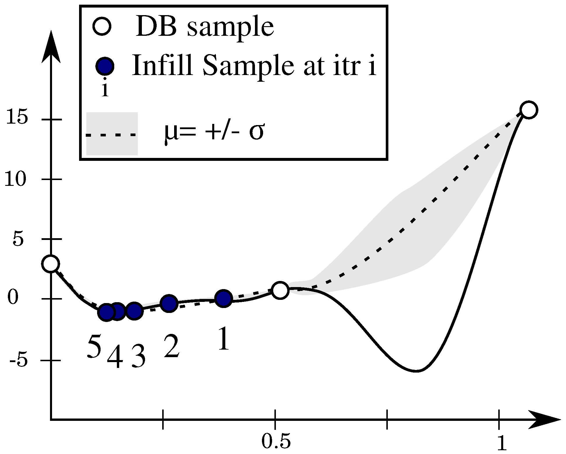
This criterion, especially suited for dense initial databases, chooses the design with the optimal prediction (e.g., minimum loss or highest efficiency). A large initial database covering well the multidimensional design space leads, in fact, to a good overall prediction accuracy. The learning is in general very effective and the metamodel-assisted optimizer converges rapidly to an optimum, which is likely to be a global one in case a global search algorithm is used.

In realistic settings, however, the initial database is not dense enough as the high-fidelity evaluation is time-consuming and the required number of design evaluations scales up exponentially with the number of design variables (curse of dimensionality). A pure exploitative infill criterion steers hence the metamodel-assisted optimizer toward a local optimum when starting from sparse data and very likely will not search in unexplored regions where a global minimum can be hidden (see Figure 1).

2.3.2. Maximum Entropy

Unlike the PM criterion, the Maximum Entropy criterion chooses the design with the maximum uncertainty or variance ${\widehat{s}}^2$ (see Equation (12)) on the prediction and does not consult the objective value.

$$s^2(x)={\widehat{\sigma }}^2(1-r{(x)}^T{R}^{-1}r(x)+\frac{1-F^T{R}^{-1}r(x)}{F^T{R}^{-1}F}).$$

(12)

The algorithm is then space-filling and works on improving the general prediction accuracy without using the system response of evaluated samples for the next infill. In practice, the metamodel-assisted optimizer with a variance maximization criterion needs many high-fidelity evaluations, especially for high-dimensional problems. Moreover, many explored areas are likely to be of low interest but need to be investigated to ensure that no potential optimum is missed, which slows down the optimizer convergence. It is more interesting to explore areas of the design space only when it is likely that they will improve the objective function. The next criterion tackles this issue.

2.3.3. Expected Improvement (EI)

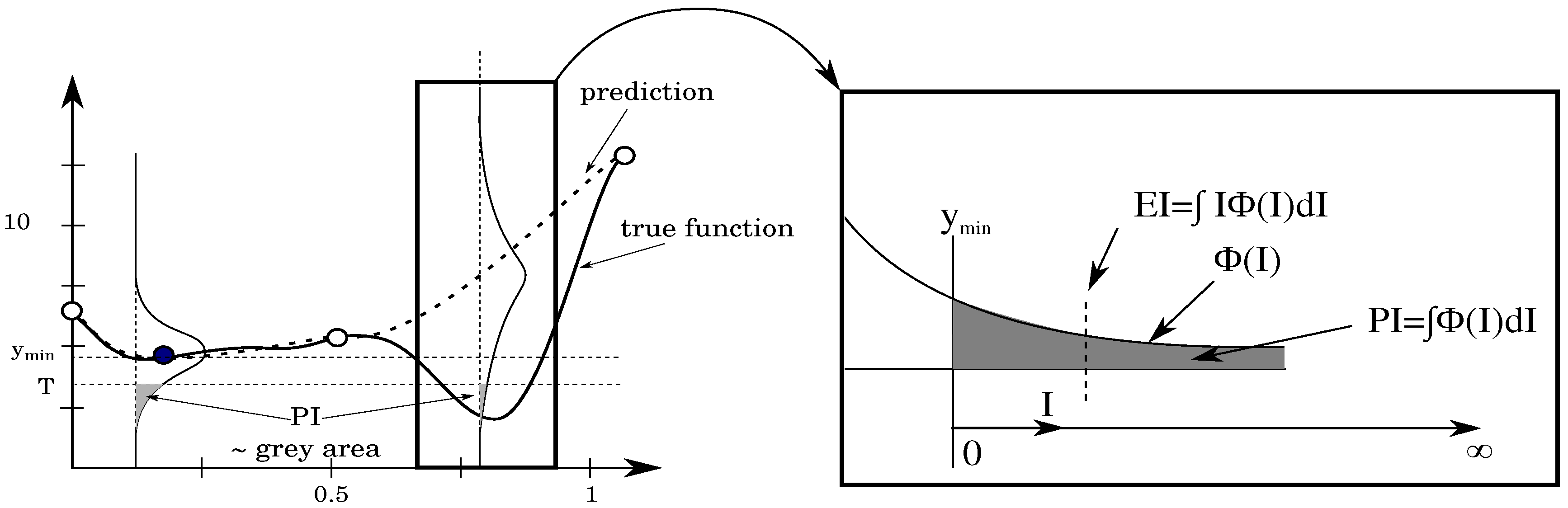
The EI criterion quantifies the expected improvement I in a certain location and the MAEA algorithm uses the information to search for the location of the highest expected improvement.

To visualize the expected improvement, one needs to look at the probability density function for a given x value, as shown in Figure 2. The mean value is given by ${\mu }_w$ while the the best value in the current set of samples is shown by $y_{min}$. The probability that the prediction is equal to y for this x value is given by:

$$\varphi (y)=\frac{1}{\sqrt{2\pi s_x}}exp(-\frac{{(y-{\mu }_x)}^2}{2s{(x)}^2}).$$

(13)

We are of course only interested in y-values that are smaller than $y_{min}$. We introduce a new coordinate axis I that starts from $y_{min}$ and goes further to smaller y-values. Each value I corresponds to a certain improvement and has a probability of improvement equal to [14]:

$$\varphi (I)=\frac{1}{\sqrt{2\pi }s}exp[-\frac{{(y_{min}-I-{\widehat{\mu }}_x)}^2}{2s{(x)}^2}]$$

(14)

The interest now goes to the mean value of I. Small values of I have a larger probability of occurring but larger values of I can still occur with significant probability if the variance $s_x$ is large. The mean value of the distribution $\varphi (I)$ is the expected improvement (EI) and is given by:

$$E(I(x))={\int }_{I=0}^{I=\infty }I\varphi (I)dI.$$

(15)

When integrated by part, the latter equation has following form:

$$E(I(x))=s[u\Phi (u)+\varphi (u)]$$

(16)

where $u=\frac{y_{min}-\widehat{\mu }}{s}$.

After rearrangement, the EI reads as follows:

$$\begin{array}{cccc}\hfill E[I(x)]& =(y_{min}-\widehat{y}(x))\Phi (\frac{y_{min}-\widehat{y}(x)}{\widehat{s}(x)})+\widehat{s}\varphi (\frac{y_{min}-\widehat{y}(x)}{\widehat{s}(x)})\hfill & \hfill & \mathrm{if}\widehat{s}>0\hfill \\ \hfill E[I(x)]& =0\hfill & \hfill & \mathrm{if}\widehat{s}=0\hfill \end{array}$$

(17)

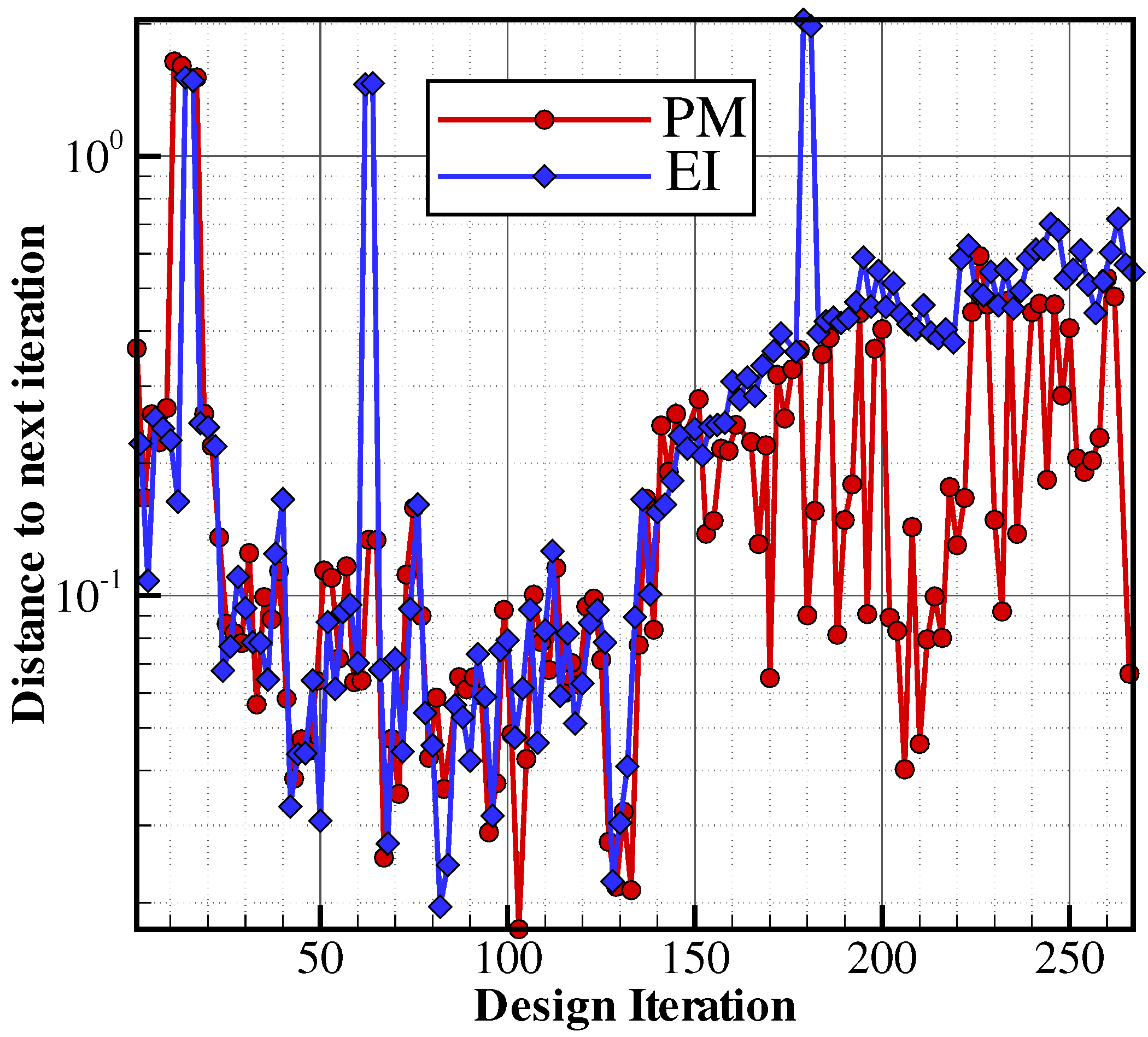
Schonlau [17] proved that EI-based metamodel-assisted optimizers can find a global optimum after a finite number of iterations. The EI value is zero at sampled locations and might increase further from samples as the variance grows. These two factors result in a multimodal shape of the EI requiring special care to find the location in the design space with the highest EI value. Figure 3 shows the convergence of the EI criterion on the Forrester function in a few iterations, unlike the prediction maximization criterion.

2.3.4. Cyclic Infill Criteria

It is possible, in a sequential optimization framework, to switch between different infill criteria during the iterative cycle. A cyclic search repeats the same cycle of acquisition, which is characterized by a number of iterations and a predefined criterion for each of these iterations. One cycle may start with few explorative samples, then gradually evolves towards fewer explorative samples and finally extremely exploitative samples, similar to Sasena [15] (p. 84). A cycle, in this work, is composed of m EI iterations followed by n PM iterations with $(m+n)$ small enough to allow multiple cycles during the optimization under limited computational budget. EI is responsible for the exploration of the design space to uncover promising regions, while the prediction minimization (PM) exploits the best design the metamodel can offer.

2.4. Treating Failed Evaluations

In a metamodel assisted optimization, the high-fidelity evaluation could be a CFD simulation, a stress analysis or any field-specific simulation. Simulations could diverge or even fail during the meshing phase, especially when challenging designs are generated or the design parameters are not properly bound. In that case, a decision has to be made on how to use the information from the failed simulation [10].

Ignoring the failed designs creates an information loss and the optimizer is likely to propose very similar designs to the failing one. When noticing the failed simulation, it is possible to push the search out of the region by an intrusive penalty strategy or a non-intrusive recovery strategy. Assigning a penalty for the objective value of the failed design masks the failure region for the optimizer, so it does not approach the same area again. The penalty distorts, however, the objective space and may hide an optimum if located next to the area of the failed simulation.

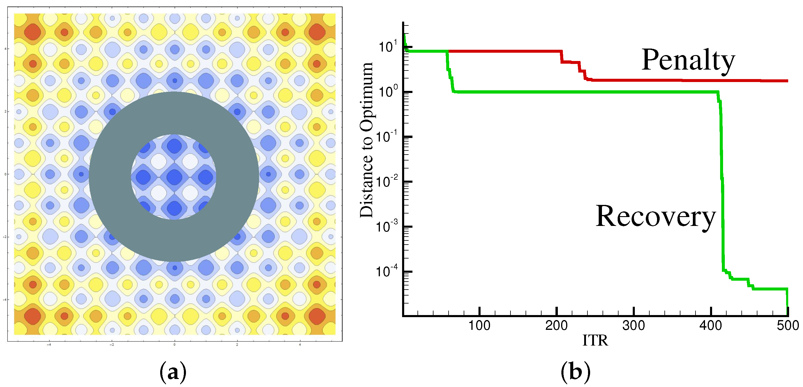
The non-intrusive strategy, on the other hand, replaces the penalty with a dummy value generated by the surrogate model [9]. Therefore, it is of utmost importance to use an explorative infill criterion, otherwise the surrogate could get trapped in an endless loop of proposing the same design which fails. The penalty and recovery approaches were tested on the Rastrigin analytical 2D function:

$$f(x)=10+\sum _{i=1}^n[x_i^2-10cos(2\pi x_i)],x_i\in [-5.12,5.12]$$

(18)

The Rasrigin function has a global shape influenced by the parabolic term $x^2$, which leads to the global optimum at $(0,0)$. The sinusoidal term creates waves on top of the parabolic shape, which render the optimization more difficult with many local optima. Moreover, the evaluation of the Rastrigin function has been slightly changed and, for certain ranges of the variables $x_1$ and $x_2$, the evaluation of the function is set artificially to fail. 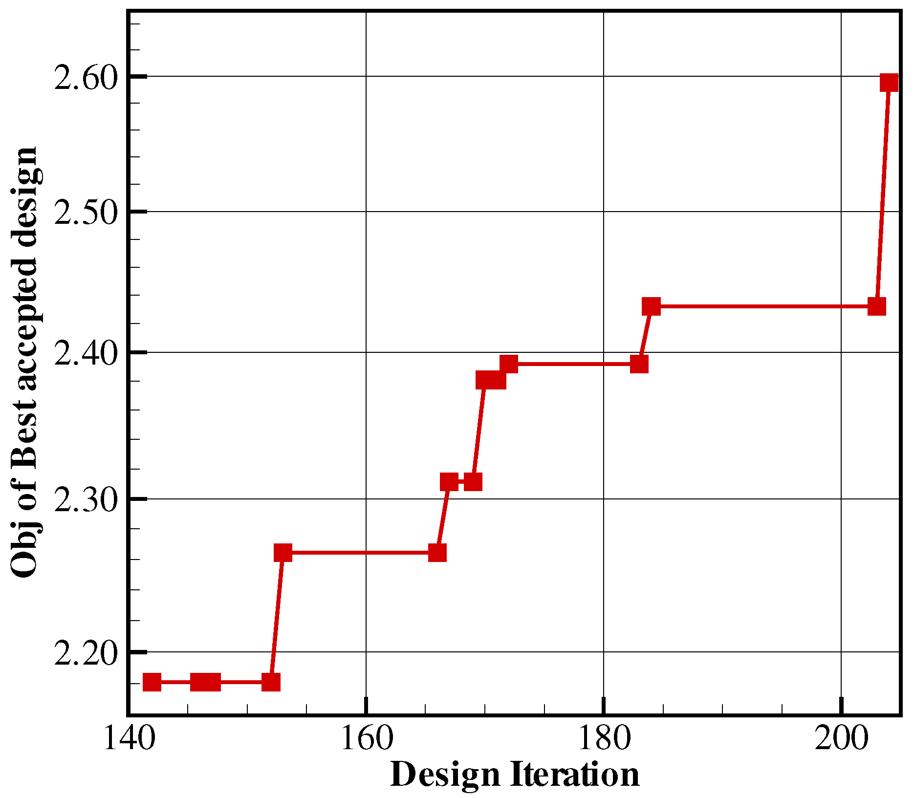Figure 4a shows a contour plot of the Rastrigin 2D function with a ring to simulate failed evaluations surrounding the optimum in the center. Both presented approaches were tested and the results are shown in Figure 4b. The penalty alternative distorts the objective space as expected and misses, therefore, the global optimum. While the penalty approach is trapped in a local minimum, the recovery approach is able to find the global optimum.

3. Application

The application is a highly constrained radial compressor for turbocharger applications. This section introduces first the geometry of the test-cases and then defines the optimization problem specifying the objectives and the constraints. Finally, the results of the meta-model assisted optimization are analyzed.

3.1. Geometry Definition and Design Variables

The 3D radial compressor is defined by:

• the meridional contour at hub and shroud (Figure 5);
• the camber line of the main blade (Figure 6a);
• the camber line of the splitter blade, as a deviation from the main blade;
• the thickness distribution for both main and splitter blade (Figure 6b); and
• the number of blades

The meridional shape of the impeller is defined by several Bézier curves or B-spline curves for both hub and shroud contours. In the present application, the contours are subdivided into three main curves: one for the inlet, one for the blade passage, and one for the diffuser. The coordinates of the control points are geometrical parameters that can be changed by the optimization program and allow to modify the meridional passage. In Figure 5, the control points that are considered as free parameters are depicted schematically by arrows. For some of the control points, the coordinates are directly controlled by the optimizer, while other coordinates are controlled by other parameters, e.g., angles and distances. This parameterization has been introduced to easily respect tangency at each interface of two patches, and to have better control on the different shapes that can be generated by the optimizer. The backplate thickness is also controlled by one degree of freedom. In total, 11 parameters control the meridional shape; for each parameter, upper and lower limits are defined.

The blade camber lines at hub and shroud are defined by the distribution of the angle $\beta (u)$ between the meridional plane m and the streamline S (Figure 6a). They are also defined by Bézier curves, where a third-order curve is used for the hub and a fourth-order is used for the shroud (see Figure 7). The camber line circumferential position $\theta$ (Figure 6a) is then defined by

$$R·d\theta =dm·tan(\beta )$$

(19)

and allows the transformation from the $\beta$ distribution to $(x,y,z)$ coordinates of the camber line provided that the meridional shape is given. In total, nine design parameters control the main blade camber line definition at hub and shroud.

When only a camber line is defined at the hub and shroud, the resulting blade will be a ruled surface and the blade can be manufactured by flank-milling. If however an additional camber line is defined in between the hub and shroud, an additional flexibility in geometry is tolerated, at the expense of a more complicated manufacturing process. In the present work, one additional camber line at the mid-section is defined. To avoid a parameterization which allows very distorted blade shapes, it is opted to define the camber line as a difference relative to the camber line that results from a ruled surface approach. Four additional design parameters control this additional flexibility.

For the splitter blade, the blade angle definition is defined relative to the main blade. A $\Delta \beta$ distribution, defined by a second-order Bézier curve, is added to the main blade $\beta$-distribution to have good control over the changes to the splitter blade. In addition, the position of the splitter blade is moved rearward relative to the main blade, which is also free within this optimization. This represents two additional design variables: one for the hub and one for the shroud. The total degrees of freedom for the splitter blade is thus 8.

The relative position of the camber line at hub and shroud needs to be defined as well. Usually, the leading edge of the hub camber line is positioned at $\theta =0$ in cylindrical coordinates. The shroud camber line can then be freely chosen relative to the hub camber line. Two possibilities exist, depending on whether the leading edge (lean) or trailing edge (rake) position is defined relative to the hub camber line. The present application uses the rake as a parameter as it is defined at a higher radius than the lean, resulting in a smaller sensitivity.

Connecting the camber lines at hub and shroud results in an infinitely thin blade on which a thickness distribution is added at hub and shroud to reach the final blade shape. The blade thickness distributions at hub and shroud are defined by B-spline curves which define the evolution of the thickness along the camber line from leading to trailing edge. The thickness distribution is specified for hub and shroud for both main and splitter blade. The thickness at the hub is proportionally scaled by a scale factor, which constitutes an additional degree of freedom. The number of blades could also be a design parameter to be optimized but has been fixed for manufacturing reasons. This brings the total number of design parameters to 34.

The fluid and solid domains are defined by the geometrical model. For the evaluation of the geometry in terms of aerodynamics and structural mechanics, these domains need to be discretized by a finite volume and finite element grid, respectively. The fluid domain is meshed with a structured grid, while, for the solid domain, unstructured quadratic tetrahedral elements are used as a compromise between element quality and automatic meshing. First, a grid in the meridional plane from hub to shroud is generated, with a stretching near the walls. For each grid line in the meridional plane, a surface of revolution is constructed. The intersection with the blade is computed, and finally a structured grid in this surface is generated by an elliptic smoother. The collection of all grids on these meridional surfaces constructs the full 3D grid. First, the bounding surfaces are meshed by using a Delaunay mesh procedure. The interior solid grid is then constructed using a similar procedure in 3D. In Figure 8, a view on the solid and fluid grid is shown.

3.2. Geometry Evaluation

The aerothermal and stress evaluations are made in parallel. NUMECA Fine Turbo is used to calculate the aerodynamic performance of the radial compressor. A structured grid with 3M cells is used for all computations to guarantee a comparable accuracy for all the samples evaluated. All computations are non-adiabatic with specified wall temperatures. For each geometry, three CFD computations are performed in parallel for the three operating points shown in Figure 9. For Operating Points 1 and 2 near surge, the mass flow is imposed at the outlet and for Operating Point 3, which is situated near choke, the base pressure is specified.

The open-source code CalculiX is used for the stress calculation. Similar grids with 250,000 nodes and 160,000 elements are used for all samples.

The grid is refined in areas of stress concentrations, e.g., at the fillet connecting the blade to the hub. A periodic boundary condition is applied, such that only a limited part of the geometry needs to be analyzed.

3.3. Optimization Problem

Present optimization is a multi-objective multidisciplinary constrained optimization (see Figure 9). The objective consists in increasing the aerodynamic performance of the impeller, while different aerodynamic and mechanical constraints are applied.

3.3.1. Objective

The objective is to maximize the total to total efficiency of the compressor at Operating Points 1 and 2. The definition of the objective function is:

$$f(\overrightarrow{\mathbf{x}})=-(0.7{\eta }_{t{t}_{OP1}}+0.3{\eta }_{t{t}_{OP2}}),$$

(20)

with

$${\eta }_{tt}=\frac{T_{2t_{i}s}-T_{1t}}{T_{2t}-T_{1t}}.$$

(21)

3.3.2. Constraints

Several constraints are imposed. The first constraint considers the maximum von Mises stresses due to the centrifugal forces in the compressor and is activated if the stress exceeds a defined material constant. Figure 10 shows the von Mises stress inside the impeller for a particular geometry. Other mechanical constraints, related to the mass and inertia of the impeller, the position of the gravity center (not too far from the supporting bearings) and the radial displacement of the blades due to the centrifugal forces, are not important in the present application and have no corresponding constraint.

$$g_1(\overrightarrow{\mathbf{x}})={\sigma }_{max}-{\sigma }_{allowable}<0$$

(22)

A second constraint concerns the choke mass flow. At low back pressure, the impeller needs to be able to deliver a minimum mass flow imposed by the manufacturer. The chocking mass flow is determined from the CFD computation at Operating Point 3.

$$g_2(\overrightarrow{\mathbf{x}})={\dot{m}}_{choke}-{\dot{m}}_{desired}<0$$

(23)

The third constraint requires that, for Operating Point 2, which uses a mass flow boundary condition, the desired pressure ratio is reached. This is necessary because otherwise, the optimizer will unload the blades to reach higher efficiency, and thus reduce the work of the compressor.

$$g_3(\overrightarrow{\mathbf{x}})={\pi }_{Req}-{\pi }_{OP2}<0$$

(24)

A fourth constraint is imposed on the momentum of inertia I, which needs to be limited to allow for good transient behavior of the rotor. The momentum of inertia is computed from the solid mesh.

$$g_4(\overrightarrow{\mathbf{x}})=I-I_{Req}<0$$

(25)

3.4. Results

In total, 129 designs were generated by the DOE process to build the initial database for the metamodel-assisted optimization. For each design, a stress analysis and three CFD evaluations were evaluated, with two CFD evaluations for the efficiency at Operating Points 1 and 2 and a third at Operating Point 3 for the choking massflow. The DOE algorithm checked the results of the designs evaluation for consistency and designs for which the evaluation was not successful (e.g., diverging CFD, meshing problems) were automatically removed. In the current case, only a few designs were rejected. It is worth to note that, in the initial database, not a single design satisfied all constraints.

The ordinary Kriging proposed a list of designs for which the CFD at Operating Point 3 was failing. therefore all results below belong to the metamodel-assisted optimization using the proposed bounded Kriging. For each optimization, two Kriging models were devoted to predicting the efficiency at Operating Points 1 and 2, necessary for the objective, and four other Kriging models were used to predict the constraints. The training used the Maximum Likelihood Estimation (MLE) and a gradient-based method (L-BFGS) was used to maximize the likelihood. For this test case, Kriging used the cyclic infill criterion explained in Section 2.3.4: for one iteration, the DE searched for the design maximizing the prediction of the compressor efficiency and for the next the DE searched for the prediction maximizing the Expected Improvement (EI) of the efficiency.

Figure 11 shows the Euclidean distance between a design and the next one of a subsequent iteration for both infill criteria when using bounded Kriging. During the search for a feasible design which satisfies all constraints, the optimizer moved slowly within the design space making small changes to the design from one iteration to the next. Once a feasibility region was found around iteration 140, the optimizer started exploring the design space, an exploration led by the EI criterion, which introduced more changes to the design, reflected in the higher Euclidean distance between designs, as shown in Figure 11.

Figure 12 shows the evolution of the bounded kriging-based prediction of the objective versus the CFD-based evaluation during the optimization. The Kriging model predicted the efficiency with an average error of 0.08% for Operating Point 1 and 0.7% for Operating Point 2. The large difference between both operating points can be explained by the higher variation in efficiency at Operating Point 2, which is located closer to surge (see Figure 9).

Figure 13 shows the evolution of the bounded Kriging-based prediction and the simulation-based evaluation for the performance parameters used to evaluate the four constraints. The relatively high prediction error of the stresses did not affect the metamodel-assisted optimizer because the stress-related constraint was satisfied early in the optimization process, as shown in Figure 13. The mass flow at OP3 rose gradually to meet the required amount after 40 iterations while the pressure ratio at OP1 took 150 iterations to reach the required threshold value. The pressure ratio at OP1, the maximum moment of inertia at OP3 and the choking massflow at OP3 were predicted with an average prediction error of 0.085%, 0.21% and 0.15%, respectively. The Von Mises stresses, however, had an average prediction error of 2.8%.

The prediction error of efficiency during the optimization shows no tendency of decline, which is related to weak learning, as depicted in Figure 12. The weak learning is due to the highly constrained problem as the optimizer explored the design space for feasibility area without intensively sampling a certain area. The optimizer searched first for designs that satisfy the four constraints before starting to improve the objective, which is confirmed by the gap appearing between prediction and CFD stating starting at iteration 145. When the feasibility area was found, the Kriging model needed to be trained to this new environment where little designs were initially present. The cyclic infill criteria also contributed to the exploratory behavior of the optimizer, which is necessary to solve such a highly constrained optimization problem.

As shown in Figure 14, an improvement of 2.59% in the efficiency was reached while the baseline design did not comply with any constraints. This proves how efficient and robust the metamodel-assisted design optimization is for highly constrained turbomachinery problems of more than 30 design variables when using bounded Kriging.

The optimized design reached lower values of entropy generation and had smaller separation bubbles, as depicted in Figure 15. The optimizer increased the thickness of both main and splitter blades to comply with the stress-related constraint. The blade loading comparison at 10% and 90% span for the baseline and the optimized designs at OP1 is shown in Figure 16. The loading near the tip increased quite substantially due to an increased turning.

The meridional contour of both designs is shown in Figure 17 along with the relative total pressure at the outlet section. The drop of the latter was proportional to the losses, which were mainly caused by the flow separation and the optimized design reached higher values of total pressure at the outlet.

4. Conclusions

This article shows the potential of metamodel-assisted algorithms for the optimization of highly constrained realistic 3D applications when using bounded Kriging. While the ordinary Kriging stopped prematurely because of a set of failing evaluations, bounded Kriging with cyclic infill was able to explore the design space efficiently and identify the area of feasible designs. After a feasible area was found, the MAEA algorithm succeeded in improving the global total-to-total efficiency by 2.59%.

References

1. Mueller, L.; Verstraete, T. Adjoint-Based Multi-Point and Multi-Objective Optimization of a Turbocharger Radial Turbine. Int. J. Turbomach. Propuls. Power 2019, 4, 10. [Google Scholar] [CrossRef]
2. Holland, J.H. Adaption in Natural and Artificial Systems; University of Michigan Press: Ann Arbor, MI, USA, 1975. [Google Scholar]
3. Matheron, G. Principles of Geostatistics. Econ. Geol. 1963, 58, 1246–1266. [Google Scholar] [CrossRef]
4. Toal, D.J.; Keane, A.J. Efficient multipoint aerodynamic design optimization via cokriging. J. Aircr. 2011, 48, 1685–1695. [Google Scholar] [CrossRef]
5. Brooks, C.J.; Forrester, A.; Keane, A.; Shahpar, S. Multi-fidelity design optimisation of a transonic compressor rotor. In Proceedings of the 9th European Conf. Turbomachinery Fluid Dynamics and Thermodynamics, Istanbul, Turkey, 21–25 March 2011. [Google Scholar]
6. Martin, J.D.; Simpson, T.W. Use of Kriging Models to Approximate Deterministic Computer Models. AIAA J. 2005, 43, 853–863. [Google Scholar] [CrossRef]
7. Bellary, S.A.I.; Samad, A.; Couckuyt, I.; Dhaene, T. A comparative study of kriging variants for the optimization of a turbomachinery system. Eng. Comput. 2016, 32, 49–59. [Google Scholar] [CrossRef]
8. Toal, D.J. A study into the potential of GPUs for the efficient construction and evaluation of Kriging models. Eng. Comput. 2016, 32, 377–404. [Google Scholar] [CrossRef]
9. Forrester, A.; Keane, A. Engineering Design via Surrogate Modelling: A Practical Guide; John Wiley & Sons: Hoboken, NJ, USA, 2008. [Google Scholar]
10. Stork, J.; Friese, M.; Zaefferer, M.; Bartz-Beielstein, T.; Fischbach, A.; Breiderhoff, B.; Naujoks, B.; Tušar, T. Open Issues in Surrogate-Assisted Optimization. In High-Performance Simulation-Based Optimization; Springer: Berlin/Heidelberg, Germany, 2020; pp. 225–244, in press. [Google Scholar]
11. Kostrewa, K.; Alsalihi, Z.; Van den Braembussche, R.A. Optimization of Radial Turbines by Means of Design of Experiment; Tech. Rep. VKI-PR-2003-17; von Karman Institute for Fluid Dynamics: Sint-Genesius-Rode, Belgium, 2003. [Google Scholar]
12. Williams, C.K.; Rasmussen, C.E. Gaussian Processes for Machine Learning; MIT Press: Cambridge, MA, USA, 2006; Volume 2. [Google Scholar]
13. Sacks, J.; Welch, W.J.; Mitchell, T.J.; Wynn, H.P. Design and analysis of computer experiments. Stat. Sci. 1989, 4, 409–423. [Google Scholar] [CrossRef]
14. Jones, D.R. A taxonomy of global optimization methods based on response surfaces. J. Glob. Optim. 2001, 21, 345–383. [Google Scholar] [CrossRef]
15. Sasena, M.J. Flexibility and Efficiency Enhancements for Constrained Global Design Optimization with Kriging Approximations. Ph.D. Thesis, University of Michigan, Ann Arbor, MI, USA, 2002. [Google Scholar]
16. Aissa, M.H.; Mueller, L.; Verstraete, T. Optimization of a turbine inlet guide vane by gradient-based and metamodel-assisted methods. Int. J. Comput. Fluid Dyn. 2019, in press. [Google Scholar]
17. Schonlau, M. Computer Experiments and Global Optimization; University of Waterloo: Waterloo, ON, Canada, 1997. [Google Scholar]
Figure 1. Minimization of the Forrester function with Minimal Prediction (MP) criteria. The algorithm is trapped in a local optimum.
Ijtpp 04 00035 g001
Figure 2. Visualization of the EI using the probability density function at position x.
Ijtpp 04 00035 g002
Figure 3. Minimization of the Forrester function using the Expected Improvement (EI) infill criteria. The algorithm finds the global optimum.
Ijtpp 04 00035 g003
Figure 4. Penalty versus recovery: (a) Adapted Rastrigin case; and (b) Convergence history.
Ijtpp 04 00035 g004
Figure 5. Geometry definition of the hub and shroud meridional flow path highlighting some design variables related to the geometry.
Ijtpp 04 00035 g005
Figure 6. Geometry definition of the camber line by a beta distribution and the blade thickness of a radial compressor: (a) camber line definition; and (b) blade thickness definition.
Ijtpp 04 00035 g006
Figure 7. Beta distribution for the main blade hub (red) and shroud (black).
Ijtpp 04 00035 g007
Figure 8. View on the mesh for both fluid and solid domains.
Ijtpp 04 00035 g008
Figure 9. The considered three operating points shown on a performance map.
Ijtpp 04 00035 g009
Figure 10. Von Mises stresses due to centrifugal forces in the impeller.
Ijtpp 04 00035 g010
Figure 11. Euclidean distance to next design of subsequent iteration for both the explorative infill (EI) and the exploitative one (PM) when using bounded Kriging.
Ijtpp 04 00035 g011
Figure 12. Comparison of the CFD-based and bounded Kriging-based predictions for the efficiency improvement at every iteration relative to the baseline design.
Ijtpp 04 00035 g012
Figure 13. Plot of the simulated against predicted constraint values for bounded Kriging: the constraint gradually being satisfied and baseline design violating all constraints.
Ijtpp 04 00035 g013
Figure 14. Best design satisfying all constraints during the optimization with bounded Kriging.
Ijtpp 04 00035 g014
Figure 15. Entropy contours and streamlines of baseline and optimized designs.
Ijtpp 04 00035 g015
Figure 16. Isentropic Machnumber of both blade and splitter for baseline and optimized design at Operating Point 1: (a) baseline; and (b) optimized.
Ijtpp 04 00035 g016
Figure 17. Comparison of baseline and optimized design: (left) the meridional contour; and (right) the relative total pressure at outlet section.
Ijtpp 04 00035 g017