Three-Dimensional CFD Simulation and Experimental Assessment of the Performance of a H-Shape Vertical-Axis Wind Turbine at Design and Off-Design Conditions ^†

Abstract

The paper presents the results of a computational study on the aerodynamics and the performance of a small-scale Vertical-Axis Wind Turbine (VAWT) for distributed micro-generation. The complexity of VAWT aerodynamics, which are inherently unsteady and three-dimensional, makes high-fidelity flow models extremely demanding in terms of computational cost, limiting the analysis to mainly 2D or 2.5D Computational Fluid-Dynamics (CFD) approaches. This paper discusses how a proper setting of the computational model opens the way for carrying out fully 3D unsteady CFD simulations of a VAWT. Key aspects of the flow model and of the numerical solution are discussed, in view of limiting the computational cost while maintaining the reliability of the predictions. A set of operating conditions is considered, in terms of tip-speed-ratio (TSR), covering both peak efficiency condition as well as off-design operation. The fidelity of the numerical predictions is assessed via a systematic comparison with the experimental benchmark data available for this turbine, consisting of both performance and wake measurements carried out in the large-scale wind tunnel of the Politecnico di Milano. The analysis of the flow field on the equatorial plane allows highlighting its time-dependent evolution, with the aim of identifying both the periodic flow structures and the onset of dynamic stall. The full three-dimensional character of the computations allows investigating the aerodynamics of the struts and the evolution of the trailing vorticity at the tip of the blades, eventually resulting in periodic large-scale vortices.

1. Introduction

Today, converting wind energy into electricity is one of the most relevant renewable technologies, and the available predictions of the energy scenario for the next 30 years agree in forecasting a further growth of electricity generation by wind turbines. To sustain such growth, on-shore wind-farm installations will not be enough and wind energy will have to be harvested in environments still exploited in a minimal part, such as large or very large scale installations in deep-sea off-shore sites, as well as mini and micro distributed generation. These contexts involve important technical difficulties (floating foundations, small-scale rotors, highly turbulent urban wind shear) that may imply a change in the design paradigm of future wind turbines. Horizontal axis wind turbine (HAWT) technology dominates the market today but, in the aforementioned non-conventional environments, the Vertical-Axis Wind Turbine (VAWT) can be an interesting alternative, for several reasons: it is inherently ’aerodynamically’ robust to yawed and skewed flows; it can provide a proper structural coupling with floating foundations (as demonstrated in the frame of the DeepWind EU program, [1]); it is characterized by lower costs of installation and maintenance as the gearbox and the generator can be placed on the ground; it produces lower acoustic pollution due to the lower optimal tip speed ratio with respect to HAWT. However, VAWT rotors are characterized by very complex aerodynamics, inherently unsteady, and fully three-dimensional, resulting in periodic fluctuating forces which ultimately complicate the structural design and affect the turbine performance.

Several engineering methods were specifically developed for VAWTs, such as the multiple stream-tube and the double multiple stream-tube, that are analyzed in detail in [2]. In recent years, higher fidelity methods based on Computational Fluid Dynamics (CFD) have been applied to VAWTs, obtaining physically-sound representations of the flow field around the rotor [3,4,5,6,7], as well as quantitatively reliable performance estimates [8]. However, such simulations cause very high computational cost that has historically led the researchers to employ simplified actuator-line [9] or 2D flow models, with proper correction terms added to account for strut and tip losses. The actuator-line approach is used in combination with LES in [10] to investigate long distance wake evolution.

From the technical perspective, simplified models still capture relevant physical effects, such as dynamic stall and the evolution of the wake, but do not allow investigating crucial features, such as the aerodynamic effect of struts, the trailing vortices and related tip losses, the span-wise flow divergence due to turbine, and wake blockage effect. With the aim of constructing a high-fidelity simulation tool for VAWTs, the formulation of a 3D CFD model causing technically-acceptable computational costs still remains a relevant challenge.

To the authors’ best knowledge, only few 3D studies have been published on VAWT simulations. 3D URANS results of VAWT in skewed flows are presented in [11], 2D and 3D models are applied in [3] for aerodynamic modeling, and in [12] to investigate the self-starting capability of VAWT. The most advanced attempt of a fully 3D simulation of a VAWT is reported in [13], where a single-blade configuration was considered due to restrictions in computational cost.

The present paper shows how a proper computational set-up allows obtaining reliable three-dimensional prediction of the flow around the rotor, of the wake, and of the turbine performance, at a reasonable (namely, industrially affordable) computational cost. Simulations were performed with the STAR-CCM+ commercial code, and the results were assessed against experimental data coming from a wide test campaign performed in a large-scale wind tunnel. A further set of 2D simulations was performed with ANSYS-Fluent for the sake of confirming that our outcomes are of general validity, using the same flow model, numerical scheme, and convergence criteria used for the main set of calculations.

The core of the paper is the detailed investigation of the three-dimensional aerodynamics of the VAWT rotor and of its wake, which is made possible by the combination of both numerical and experimental large databases.

The paper initially introduces the physical models and the numerical schemes. The following analysis of the VAWT flow field is done at two levels: firstly, the rotor aerodynamics is discussed in connection to the computed and measured performances; then, the unsteady evolution of the three-dimensional wake is considered, also in comparison to corresponding experimental data. Conclusions are then drawn on the most relevant flow structures, in view of performance improvement at design and off-design operation.

2. Case Study: Turbine Model and Experiments

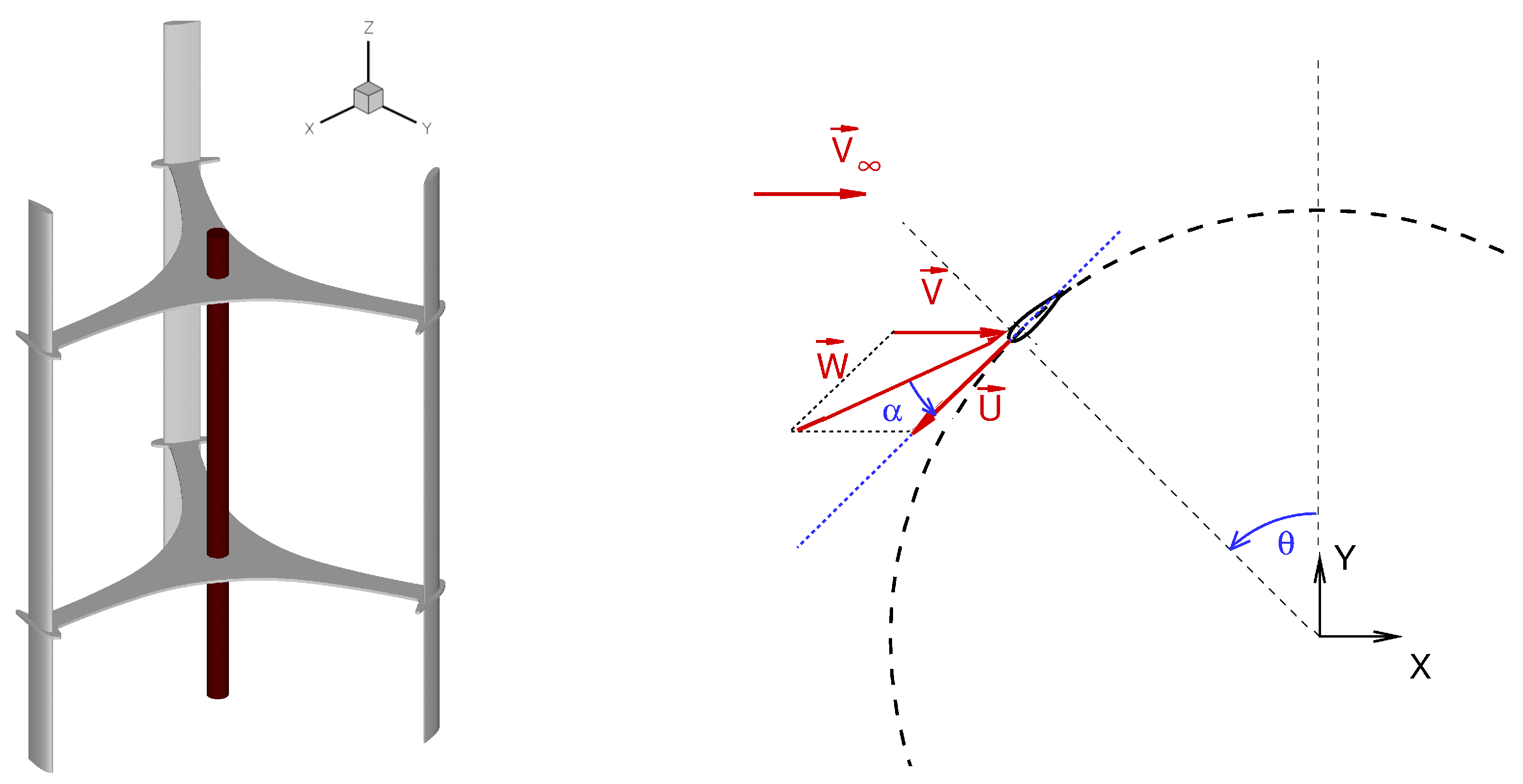
This study focuses on a model turbine representative of a real-scale VAWT for micro-generation ($P_{max}$ = 200 W). The rotor features a straight H-shape and consists of three unstaggered blades; see Figure 1 which displays the turbine configuration along with the coordinate system and the relevant angles. The main geometrical characteristics of the turbine considered are reported in

Table 1. Vertical-Axis Wind Turbine (VAWT) geometric parameters.

Blade height	1.457 m
Rotor diameter	1.030 m
Solidity	0.25
Chord	0.086 m
Blade airfoil	NACA0021

. Full details on the turbine geometrical features, as well as on the turbine operating and performance parameters, can be found in [14].

In the present study, two operating conditions are considered, one close to the peak $C_p$ condition and one at higher tip speed ratio (TSR). Coherently with the experiments, the turbine operates at constant angular speed of 400 rpm and the different TSR conditions are obtained by varying the wind speed. The Reynolds number based on the peripheral velocity and the airfoil chord is therefore constant among the different conditions and amounts to $1.2\times {10}^5$. The details of the conditions considered and the related performance obtained in dedicated wind-tunnel experiments are reported in

Table 2. Working conditions.

V${}_{\mathit{\infty }}$ [m/s]	Tip-Speed-Ratio (TSR)	${\mathit{C}}_{\mathit{P}}$	${\mathit{U}}_{{\mathit{C}}_{\mathit{P}}[95\%]}$
6.54	3.3	0.16	0.03
9.00	2.4	0.27	0.02

. Different levels of uncertainty resulted for the two TSRs, due to the different values of the measured quantities compared to full-scale.

The performance and the wake shed by the turbine were characterized experimentally in open-chamber, free-jet configuration, the jet being of square cross area of about 16 m${}^2$ with the rotor placed in the center of the jet. The application of dedicated correlations [15] indicates a negligible free-blockage. The incoming flow features very low turbulence (below 1%). Performance measurements were obtained by combining angular speed with torque measurements while velocity and turbulence measurements were performed in the wake by traversing multiple hot wires. They provided time-resolved measurements of both streamwise and cross-stream velocity components with an uncertainty of about 2% of the local velocity value. A proper data-processing technique, reported extensively in [16], was performed to extract the time-averaged, the phase-resolved, and the streamwise turbulent components of the velocity.

3. Computational Flow Model

The definition of the computational flow model was conceived combining the information available in the open literature with dedicated parametric studies on specific computational aspects aimed at limiting as much as possible the computational cost of the simulations. The parametric study is documented in a recent paper of the same authors [17] and led to a novel set-up that allows performing fully 3D CFD simulations with industrially-relevant computational cost. This paper is focused on VAWT aerodynamics and, hence, only the main features of the CFD model are herein recalled.

Turbulent incompressible flow is considered, selecting the $k-\omega$ SST model developed by Menter [18] to account for the effects of turbulence. For such small-scale VAWT application, the low-Reynolds correction of the turbulence model is of interest and it was the object of a dedicated investigation in the present study, as discussed later. It consists in a modification of the model coefficients, in order to account for natural transition effects in a computationally efficient way, introduced by Wilcox in 1994 [19] and fully described in both Fluent and STAR-CCM+ user guides.

The discretization employed is second-order accurate both in space and time and the solution of the unsteady RANS equations was carried out using a constant time step. In particular, while a time step corresponding to 0.5 deg of revolution was enough for TSR = 3.3, for TSR 2.4 a reduced time step, corresponding to 0.25 deg of revolution, showed necessary to achieve time-step independence.

The solution of the discrete problem is achieved using the pressure-based coupled algorithm for the momentum and the pressure correction equations, while the turbulence model equations are solved in a decoupled way. The nonlinear system arising at each time step is solved using an algebraic multigrid solver up to an accuracy level of ${10}^{-5}$ measured by the norm of scaled residuals. Convergence of the computations is instead evaluated by monitoring the time variation of the power coefficient, and searching for a periodic time-evolution. Fifteen-to-twenty turbine revolutions were needed to obtain a fairly good periodic solution. The root mean square of the power coefficient (based on the computation of the average $C_P$ value in each of the last eight revolutions) is less than $1\%$ of its mean value. This value exactly matches the experimental uncertanity.

The above description holds for both the solvers applied in this study.

The computational domain is composed of two parts: an inner region, which defines the discretization of the moving part (the turbine with the shaft and the airfoil sections) and an outer area, which defines the far field and the far wake region. The sliding mesh technique is used to deal with the turbine rotation.

As well known, an insufficient extension of the computational domain has a crucial impact on the wind turbine calculations. A proper placement of the inflow condition is crucial to reproduce the actual induction effect upstream of the rotor and the lateral surfaces, where most of the authors in literature apply periodic/symmetry/slip-wall conditions, need to be distant from the turbine to avoid an unphysical blockage effect. Normally, in VAWT 2D simulations, the domain extends for ten-to-twenty rotor diameters upstream, downstream, and on both the sides of the turbine, thus leading to a very heavy computational burden if such extension is maintained in the 3D framework. To tackle such a cost, a recent study has been performed by the authors [17] on the impact of the domain extension in combination with the set of boundary conditions. The main results of that analysis are here briefly recalled. At first, the use of pressure boundary conditions on the lateral surfaces strongly reduces the blockage effect, and it allows limiting the lateral domain extension to 3 rotor diameters on both the lateral sides of the rotor. The inlet boundary is, instead, more critical, but its criticality was found to be mainly a by-product of a 2D discretization. When 3D calculations are performed, the degree of freedom available in vertical (i.e., axial) direction allows the flow to pass over the rotor, drastically reducing the artificial blockage observed in the 2D simulations. Eventually, a distance of 4.5 rotor diameters upstream of the turbine was found to be enough to perfectly match the blockage observed in the experiments. The static pressure was also assigned 3 diameters downstream. 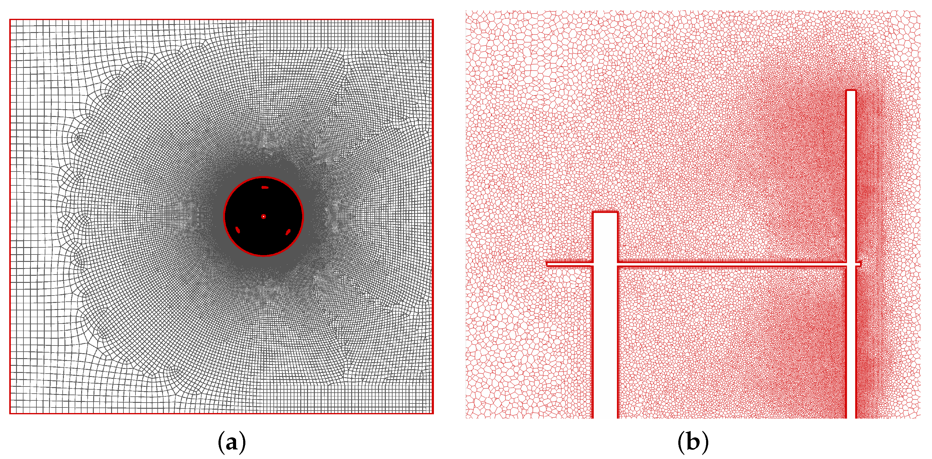Figure 2 shows the domain and the computational mesh. By using such computational set-up, a typical 3D simulation carried out using Star-CCM+ on a 16-processors (Intel Xeon E5 2.3 Ghz) parallel cluster took approximately 24 days and required 37 GBytes of core memory.

In the early stages of this work, a grid convergence study was performed related to both the near-wall region and the global resolution level, documented in [17]. The study was performed for the 2D mesh on the equatorial plane at TSR = 3.3. In all the tested meshes, as the selected turbulence model allows solving entirely the flow in the boundary layer, the near-wall space discretization fulfills the requirements of $y^{+}\approx 1$ and of a smooth growth across the boundary layer. On the basis of these considerations, a base grid was then constructed and is shown in Figure 2a. It consists of 253.800 cells (40.000 out of them are in the outer region), with a minimum distance from solid walls of $2\times {10}^{-2}$ mm and a local growing factor of the boundary layer of 1.2. To assess the influence of global mesh density, tests were run with two finer meshes featuring, alternatively, the double number of elements and half the cell size at the walls. Both these tests did not show any significant difference with respect to the base grid, which was therefore considered suitable for obtaining a grid-independent solution (see Table 3 of [17]).

When focusing on the 3D case, the computational domain was obviously retained; concerning the domain extension in the axial direction, only half of the turbine height was considered, imposing a symmetry condition on the equatorial plane; on the top side, the domain was extended above the blade tip by slightly more than 50% of the half-span of the blade (the distance between equatorial plane and blade tip). Such a configuration was found to be sufficient to eliminate any spurious overestimation of the blockage effect in 3D calculations. The 3D meshes have been generated following the guidelines defined in the 2D computations and similar grid spacings have been employed, although regions far enough from blade surfaces were made coarser in order to save computational resources. Out of the near wall regions both grids are of polyhedric type; by virtue of this choice the total number of elements (and hence the RAM storage requirement) is greatly reduced (about eight million cells), even if the number of faces is still sufficiently high to guarantee a good numerical resolution, as demonstrated by the results presented in the following. A cut-plane showing the distribution of cells is reported in Figure 2b.

At the inlet boundary the unperturbed flow velocity was imposed, altogether a turbulence intensity $Tu=1\%$ (the experimental value) and a viscosity ratio ${\nu }_t/\nu$ equal to one, which is a typical value adopted with this turbulence model. Ambient pressure is imposed on the lateral boundaries, on the top boundary above the blade tip, and at the outflow boundary.

4. Rotor Aerodynamics and Turbine Performance

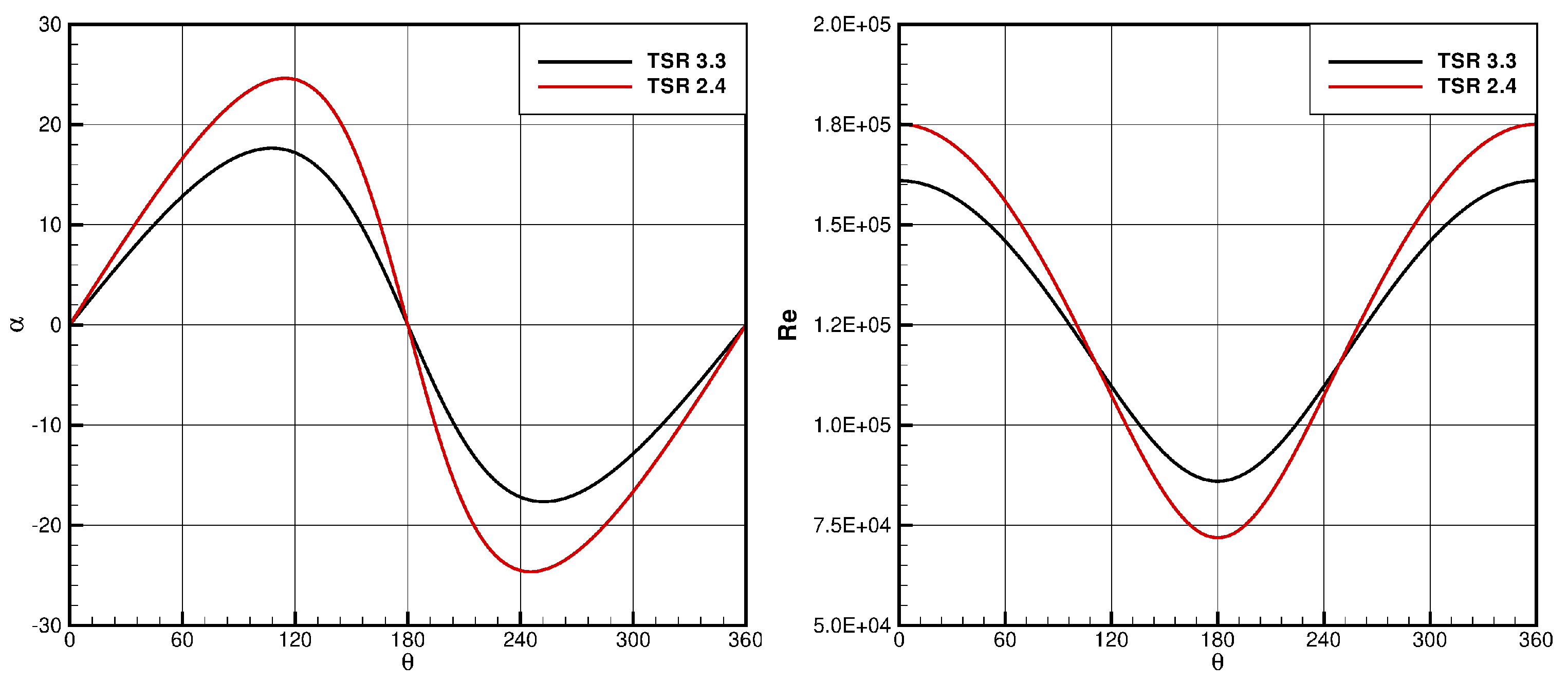
The analysis of the VAWT flow field first focuses on the rotor aerodynamics. To give an idea of the local conditions experienced by the blade during the revolution, Figure 3 shows the angle of attack and the Reynolds number (based on chord and relative velocity) profile for both TSRs studied. Note that these graphs of course neglect any induction effect, i.e., the local wind absolute velocity is the freestream one.

Instantaneous and average configurations, phase-resolved torque coefficient trends, and rotor performance data are considered to shed light on the flow mechanisms occurring in the different phases of the revolution and their influence on the generation of moment; the computed VAWT performance is also compared to experimental values to assess model reliability.

At first, calculations at high TSR (3.3) and small freestream wind have been performed using the low-Reynolds correction of the $k-\omega$ SST model.

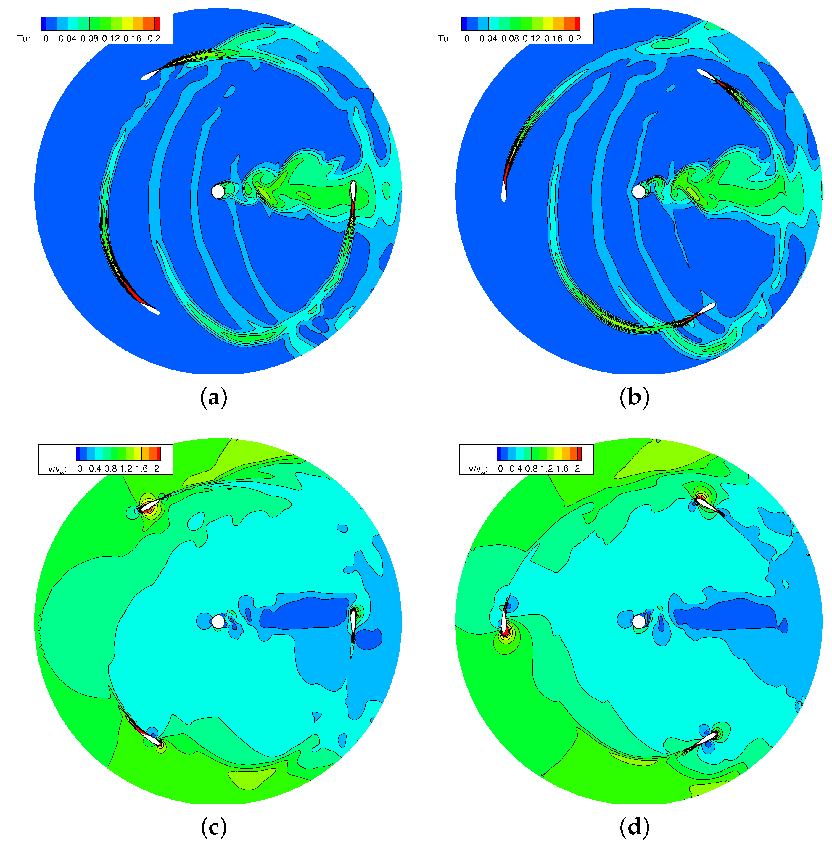
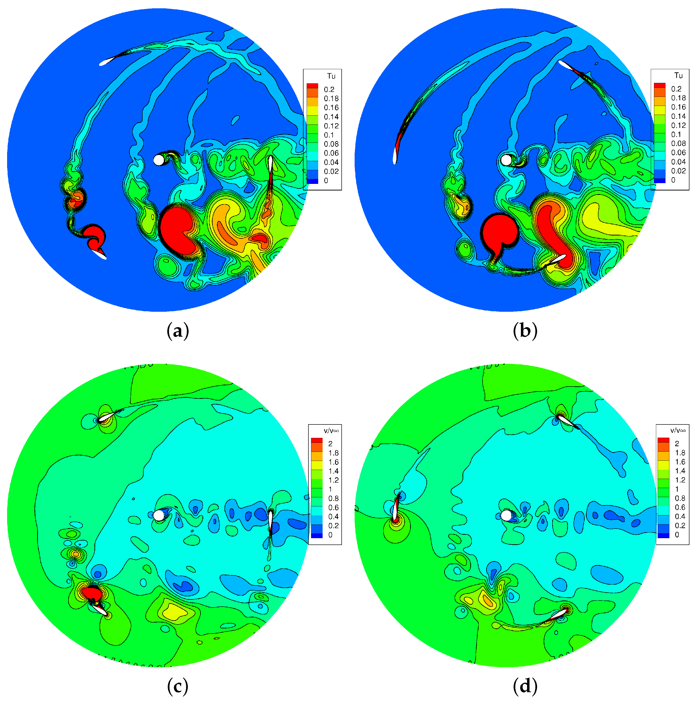
As well known, during a revolution the VAWT blades experience a cyclic variation of angle of attack and of relative Reynolds number, which induces a periodic fluctuation of blade forces. Such effects grow progressively as the TSR reduces; however, they appear even at TSR = 3.3, as shown by Figure 4, which reports instantaneous snapshots of the turbulence and velocity fields in the equatorial section of the turbine, for two rotor positions.

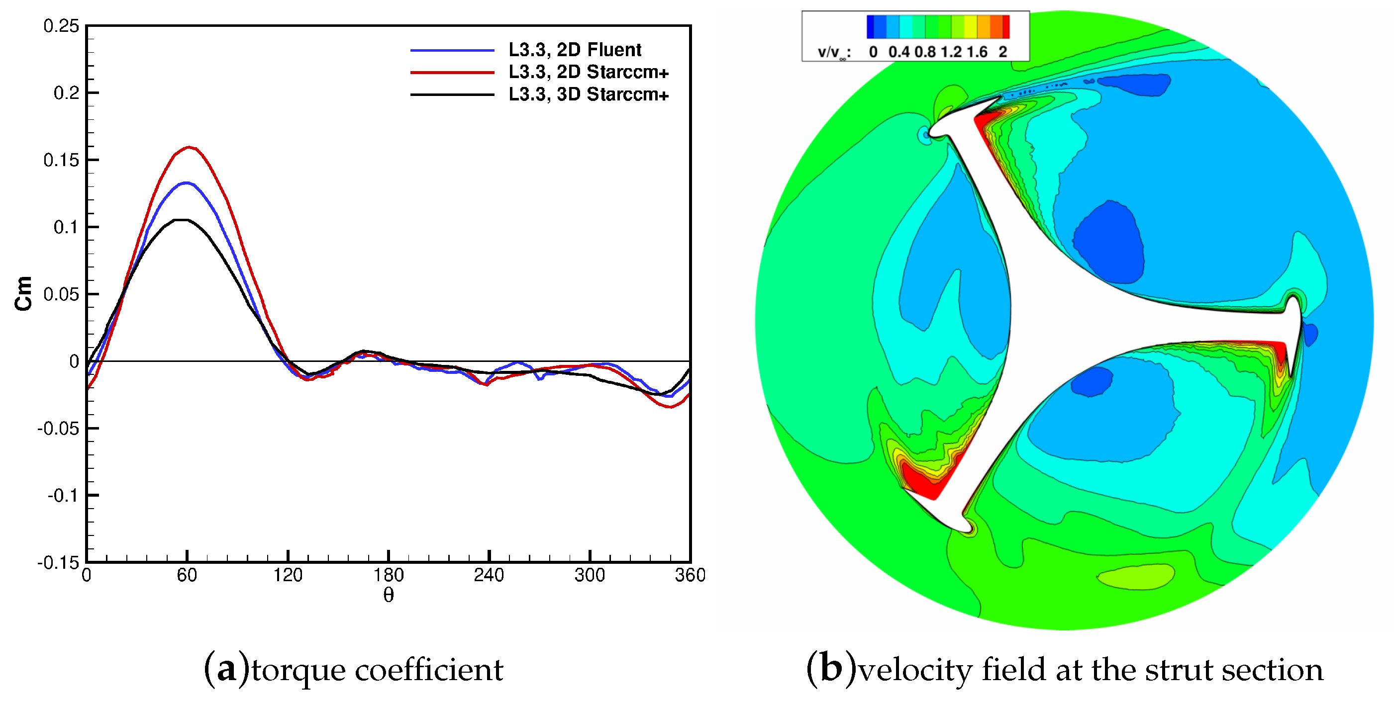
In order to highlight the connection between flow phenomena and performance, the evolution of the torque coefficient along a full blade revolution is added in Figure 5a. In this plot, the results coming from 2D simulations obtained with the two solvers, as well as the ones obtained with 3D simulations using STAR-CCM+, are considered. First considering 2D results, which exhibit coherence between the two solvers, in the upwind fraction of the revolution ${45}^{\circ }\le \theta \le {135}^{\circ }$ the blade interacts with the incoming unperturbed flow and the angle of attack progressively rises without inducing flow separation. In this period (in particular for ${20}^{\circ }\le \theta \le {120}^{\circ }$) most of the torque exchange takes place, with a peak value at $\theta \approx {70}^{\circ }$. At the end of this phase a small separation occurs in the rear part of the blade, indicating a typical post-stall airfoil configuration, even though no large-scale vortices detach from the airfoil surfaces. This corresponds to the local minimum of torque coefficient visible in the trend of Figure 5. The rise of the drag force leads to the onset of a passive torque that lasts for the entire leeward phase (${135}^{\circ }\le \theta \le {225}^{\circ }$); in this phase, the blade experiences the highest fluctuations, as well as the peak values of incidence (both positive and negative), with the only exception of a small region around $\theta ={180}^{\circ }$, where the angle of attack steeply goes to zero almost nullifying the overall torque. Moreover, as clearly visible in Figure 4, in the leeward motion the blade cuts the turbulent vortical structures released by the preceding blades. In the downwind portion of the blade revolution (${225}^{\circ }\le \theta \le {315}^{\circ }$) the torque coefficient remains zero or even negative, as the low velocity of the flow (decelerated by the interaction with the rotor in the upwind phase) combines with the high angle of attack reducing the lift at high drag; these effects are further amplified by the blade interaction with the large wake of the pole. It is interesting to note that the ANSYS-Fluent simulation predicts higher torque in the first quarter of the revolution, while adhering closely to the STAR-CCM+ simulation for the remainder of the revolution.

The torque evolution commented above remains substantially similar when 3D simulations are considered; it is interesting to note that, in the wide period of negative (resistant) of nearly null torque (${120}^{\circ }\le \theta \le {360}^{\circ }$), the 3D simulation reproduces the results of the 2D one. An evident 3D effect appears, instead, in the fraction of period featuring the highest torque (${20}^{\circ }\le \theta \le {100}^{\circ }$), where a considerably lower peak torque establishes with respect to the 2D prediction. As expected, the tip aerodynamics and the struts induce an extra drag that reduces the positive (driving) torque in the active part of the revolution. Figure 5b reports the velocity field on a plane corresponding to the struts for $\theta ={30}^{\circ }$. The struts induce a generalized reduction of flow velocity (alongside a widespread generation of turbulence, not reported for sake of brevity) even in the upwind region of the rotor.

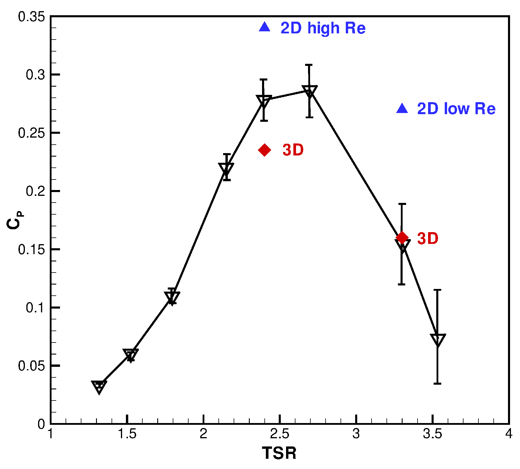
In terms of overall performance data, for TSR = 3.3 the 2D simulation predicts a Cp value of 0.23. When 3D simulations are considered, the Cp prediction drops to 0.157. This value is in excellent agreement with the measured Cp that resulted 0.16 (see Table 2), showing the technical relevance of the proposed flow model.

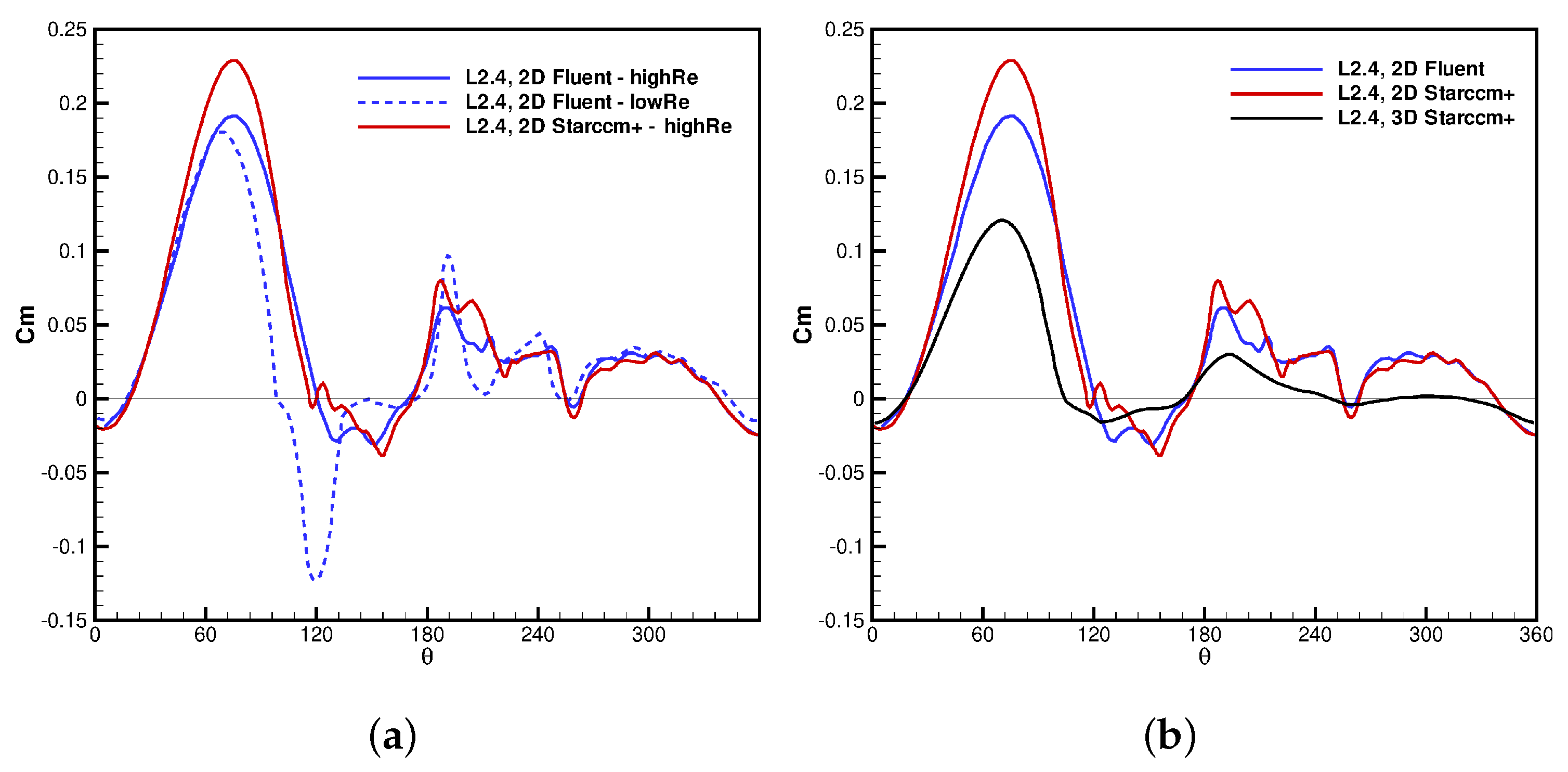
A similar set of calculations was performed for TSR = 2.4, a point close to peak efficiency condition, and the results are shown in Figure 6 and Figure 7. As clearly visible in the distributions on the equatorial plane, the flow configuration becomes much more complex when the TSR reduces, with massive separations occurring in the leeward phase of the revolution. These turbulent structures develop along the blade surface from leading edge to trailing edge and vice versa (see [20] for a classical flow scheme of dynamic stall and super-stall, aka leading-edge stall, in VAWTs). As a result of the severe stall on the blades, high passive torque is generated for $\theta \approx {120}^{\circ }$, when super stall takes place. The blade exits from stalled conditions for $\theta \approx {180}^{\circ }$, and subsequently no severe dynamic stall occurs. Despite for ${180}^{\circ }\le \theta \le {240}^{\circ }$ the blade travels in a region affected by the detachment of large-scale vortices, a positive torque is issued by the flow to the blades; after a region of torque drop when the blade travels in the wake of the pole, the torque turns to positive values for ${270}^{\circ }\le \theta \le {330}^{\circ }$.

Considering the turbine performance, the 2D simulation predicts a Cp value of 0.195, which is significantly below the experimental value of 0.27. Such an underestimation indicates reliability issues, as in a 3D calculation an even lower value is expected. The detailed analysis of the airfoil aerodynamics reveals that the low power extraction is caused by the severe drop of torque caused by the onset of super-stall at the end of the upwind phase. In fact, such effect is not consistent with the estimates of aerodynamic forces coming from the application of engineering methods (double multiple streamtube model) to this machine which, instead, led to an excellent agreement with the experimental performance [21].

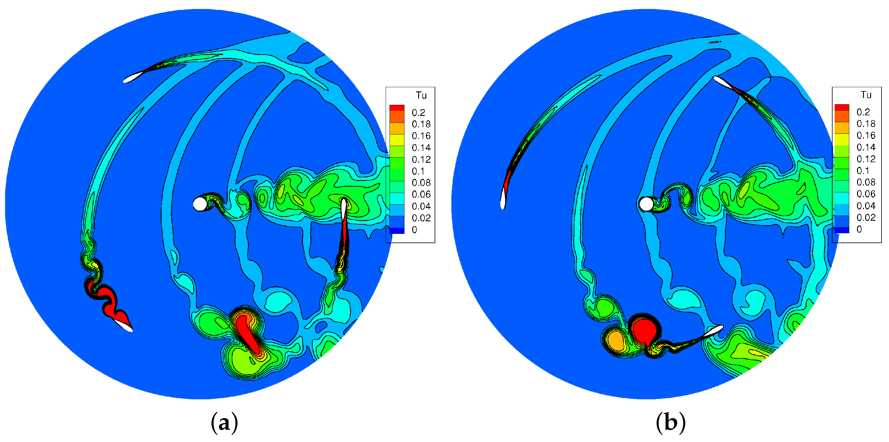
As a too severe separation is responsible for the mismatch with the experiment, a potential modeling issue was identified in the low-Reynolds formulation of the turbulence model. Simulations were then performed without such feature, and the corresponding turbulence field is reported in Figure 8. The new simulation still predicts the onset of dynamic stall at the end of the upwind phase which corresponds to a period of passive torque, but the extension of the separated region and the scale of the vortices detached by the blades are much smaller with respect to those predicted with the low-Reynolds model, shown in Figure 6. Correspondingly, Figure 7 reveals that the peak of passive torque is strongly mitigated. Differences arise also for ${180}^{\circ }\le \theta \le {240}^{\circ }$, as the much “cleaner” flow configuration predicted without the low-Reynolds correction induces a higher (active) torque. Very similar flow field and blade aerodynamics are predicted by the two simulations for ${270}^{\circ }\le \theta \le {90}^{\circ }$, where the lower angle of attack does not activate any relevant dynamic stall effect.

The generally higher torque predicted by the calculation without the low-Reynolds correction implies a net increase in the prediction of Cp value, which rises to 0.34, which is (as expected) greater than the experimental value of 0.27. As a matter of fact, the performance estimation drastically reduces in 3D calculations, which were carried out only without the low-Reynolds correction. As already observed for TSR 3.3, also for lower TSR the peak torque coefficient occurring in the upwind phase reduces significantly; moreover, the struts and tip losses contribute significantly to reduce $C_m$ also in the downwind phase, almost nullifying the slight active torque predicted in this phase by the 2D model. By virtue of the observed features, the 3D simulations estimate a Cp value of 0.235, much lower that the 2D one and, again, in good agreement with the experimental datum. Notice that the difference between 2D and 3D power coefficients rises with TSR, as tip and strut power losses are roughly proportional to the square of the peripheral velocity multiplied by the wind speed (as commonly found in helicopter blades), whilst the power scales with the cube of the freestream wind speed; hence, non-dimensional losses due to 3D effects grow with the square of the TSR.

In Figure 9 the turbine Cp values measured for all the operating TSR conditions are displayed along with the computed 2D and 3D results obtained using Star-CCM+. In

Table 3. Cp values of computations carried out with Star-CCM+ and ANSYS-Fluent using low-Reynolds and high-Reversion of the $k-\omega$ model.

TSR	$\mathit{k}-\mathit{\omega }$	2D Fluent	2D Star	3D Star
3.3	LR	0.25	0.27	0.16
	HR	0.21	0.23	–
2.4	LR	0.21	0.20	–
	HR	0.31	0.34	0.23

the computed Cp values are also reported together with those obtained with ANSYS-Fluent. These results allows to appreciate the difference between 2D predictions obtained using the $k-\omega$ model with or without the low-Reynolds correction. There is a discrepancy between the 2D Fluent and the Star-CCM+ results, due to different underlying numerics (unknown to the user), but this difference is still within a reasonable tolerance level, comparable to the uncertainty of the experimental datum and considerably smaller (even one order of magnitude lower for the TSR = 2.4) than that obtained by activating the low-Reynolds correction.

5. Three-Dimensional VAWT Wake

The analysis reported so far shed light on the contribution of three-dimensional effects on the aerodynamics and performance of VAWT rotors, and demonstrates the reliability of the computational model here proposed. However, a full analysis of a wind turbine demands a proper investigation of the turbine wake, both in terms of computational modeling and flow physics. For this reason, a dedicated analysis of the time-resolved and 3D turbine wake is now presented, in comparison to the available measurements in the near wake of the turbine.

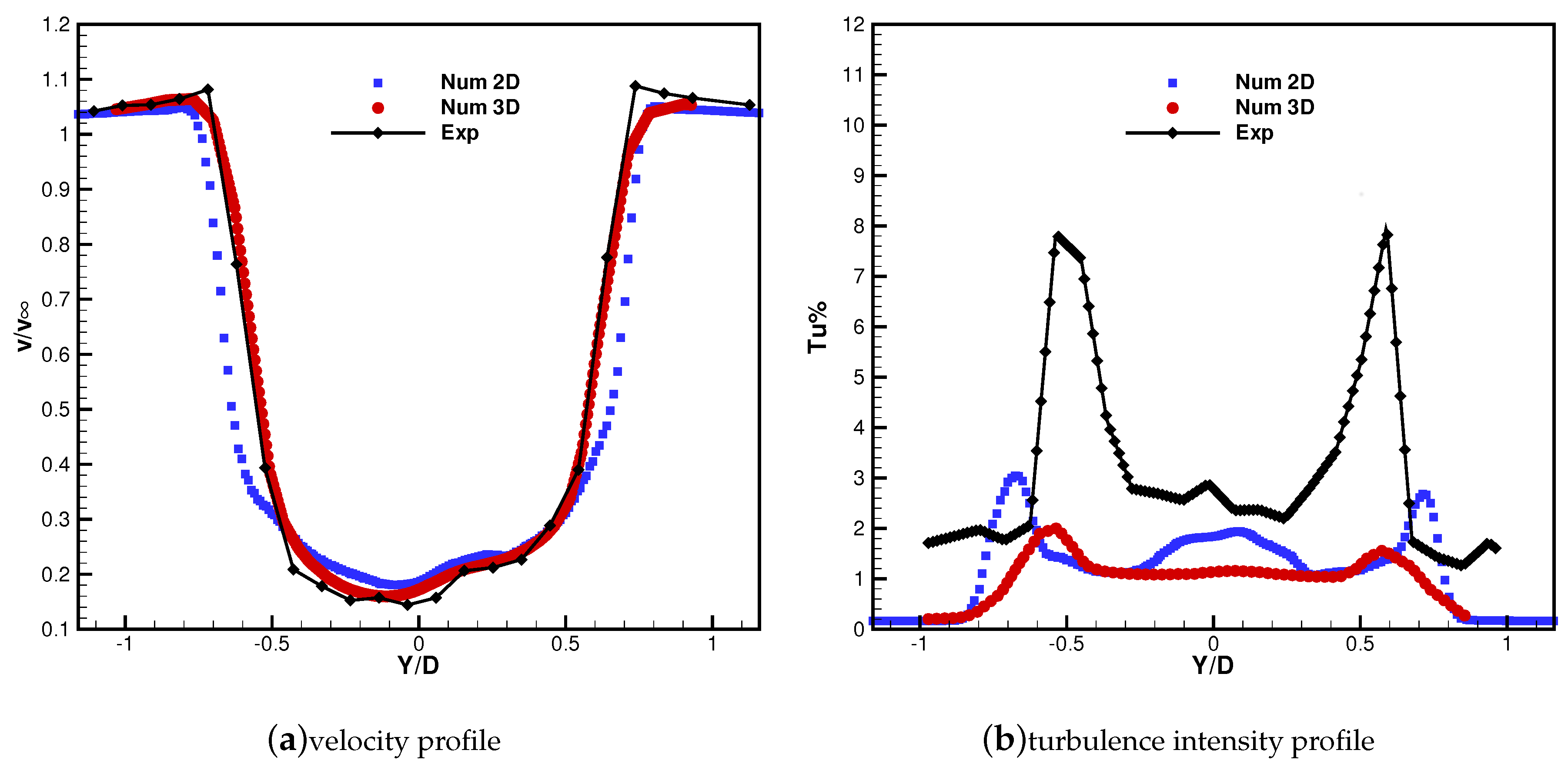
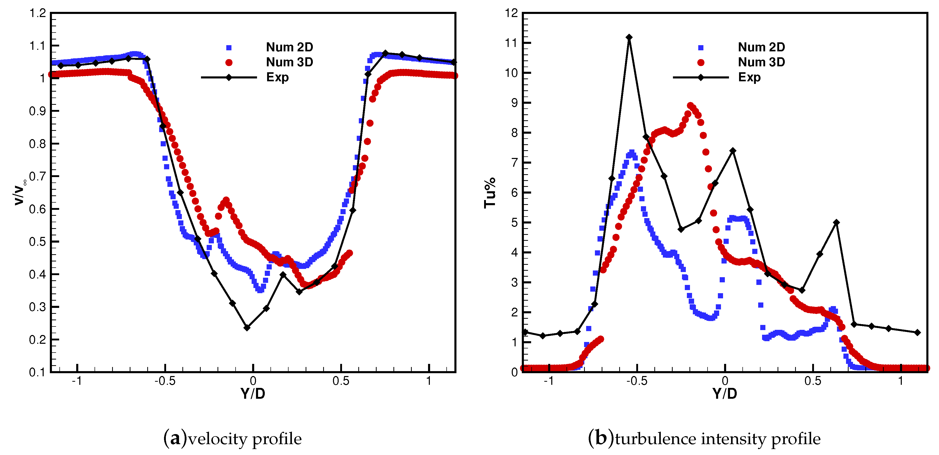
The time-averaged wake profiles on the equatorial section are first considered and are shown in Figure 10 and Figure 11 against the experimental data. The velocity profiles are found to be in very good agreement with the experiment in terms of wake width and shape. The velocity deficit, perfectly captured by the simulation for the high TSR condition, is slightly underestimated for TSR = 2.4. The profile of turbulent intensity ($Tu$) predicted by the 2D simulation, computed as $\sqrt{2k/3}/v_{\infty }$, is also compared with the experimental result. For TSR = 3.3 the trend is reproduced in acceptable manner even though the turbulence level are not captured. A similar behaviour is also observed for the 2D results obtained for TSR = 2.4. For such condition, three peaks of turbulence intensity are observed, connected to the two shear layers at the sides of the wake and to the viscous wake of the pole. This trend is well captured by the simulation, with an underestimation consistent with the fact that in the experiments $Tu$ is defined using only the $rms$ of the velocity fluctuation in the freestream direction, i.e., the greatest term, whilst in the simulations velocity fluctations are assumed isotropic. Moreover, in the experiment every unsteadiness at locked rotor angular position is considered to be turbulence. Instead, as indicated by the smeared $Tu$ profiles obtained in 3D (see Figure 7 and Figure 11), the flow gradients appear somewhat damped due to insufficient mesh resolution. As a matter of fact, the adopted grid density, slightly reduced with respect to the 2D cases, is deemed necessary to limit the computational cost at a reasonable level; however, as shown by the present results, such discretization allows obtaining reliable predictions of the turbine performance and of the wake velocity profile.

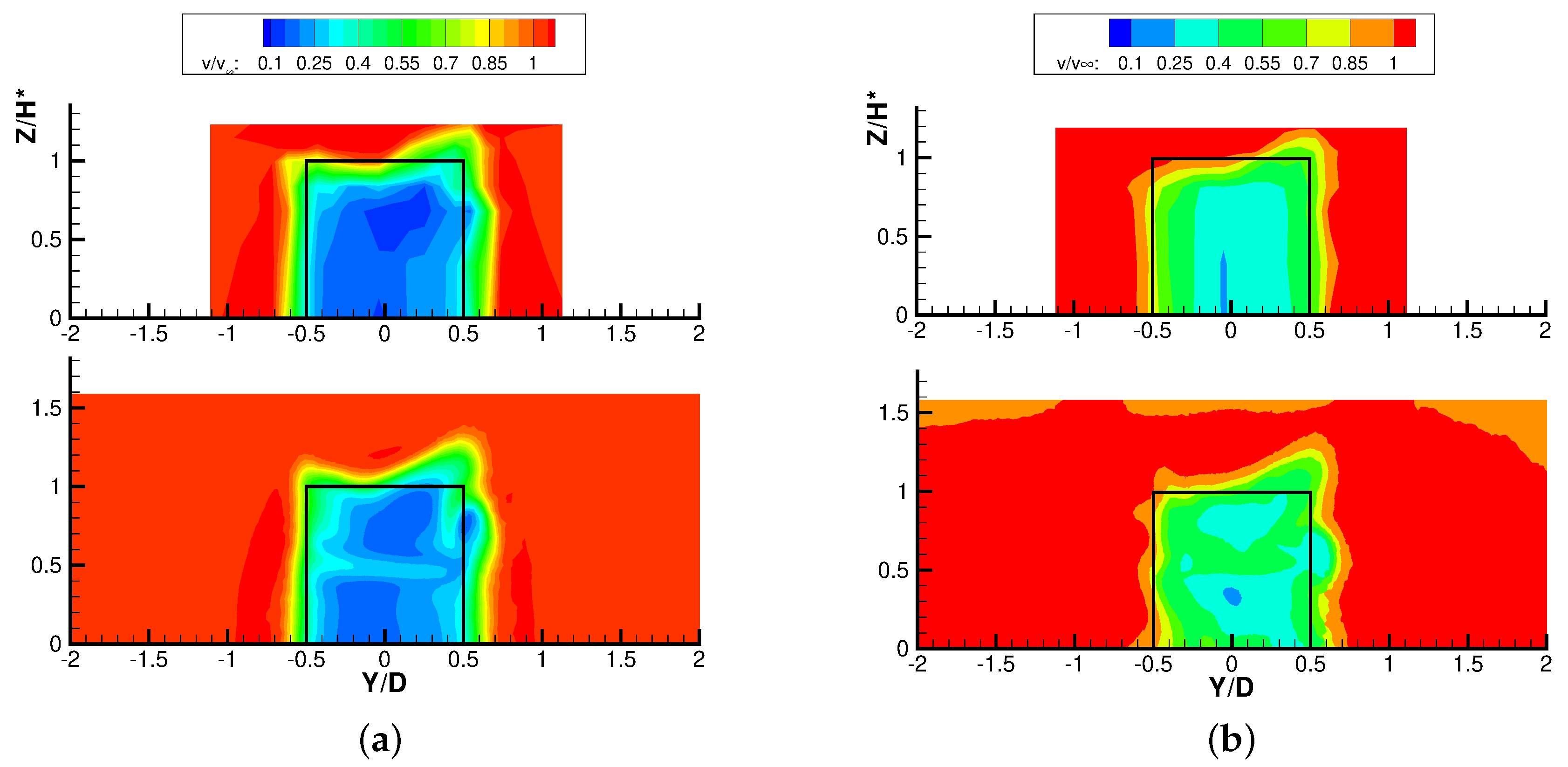
The three-dimensional character of the wake is illustrated in Figure 12 that shows the time-mean velocity contours on a surface normal to the streamwise direction at $x/D=0.75$. The shape of the wake has an evident asymmetry with respect to the shaft especially in the top quarter of span, closer to the blade tip. In fact, the asymmetry characterizes the VAWT, and the differences between the two sides of the wake result from the different flow processes occurring in the windward (on the right in the frames) and in the leeward (on the left in the frames) fractions of the revolution. As widely discussed in [22], the larger extension of the right side of the wake at the tip is due to the larger mean lift established on the blades during the windward motion, which leads to a stronger tip vortex and relevant losses. This effect grows in importance as TSR reduces, since for lower TSR the differences in blade aerodynamics between the windward and leeward motion become larger. As a result, the tip region of the wake takes an inclined shape that becomes progressively more marked during the streamwise wake development (not reported here for the sake of brevity).

The simulations show a very good agreement with the experimental velocity distribution in the wake, both in terms of wake extension and velocity deficit all along the blade span, and especially in the tip region. The unique evident difference between simulations and experiments lies in the region of lower velocity deficit at $z/H^{*}=0.5,$ where $H^{*}=H/2$. However, such difference is only apparent: This local perturbation is indeed an effect of the struts that are placed exactly at this spanwise position; for limitations in the measurement time (the focus was on the equatorial and on the tip regions), the experimental mesh is not refined enough in this area to properly capture the effect of the struts.

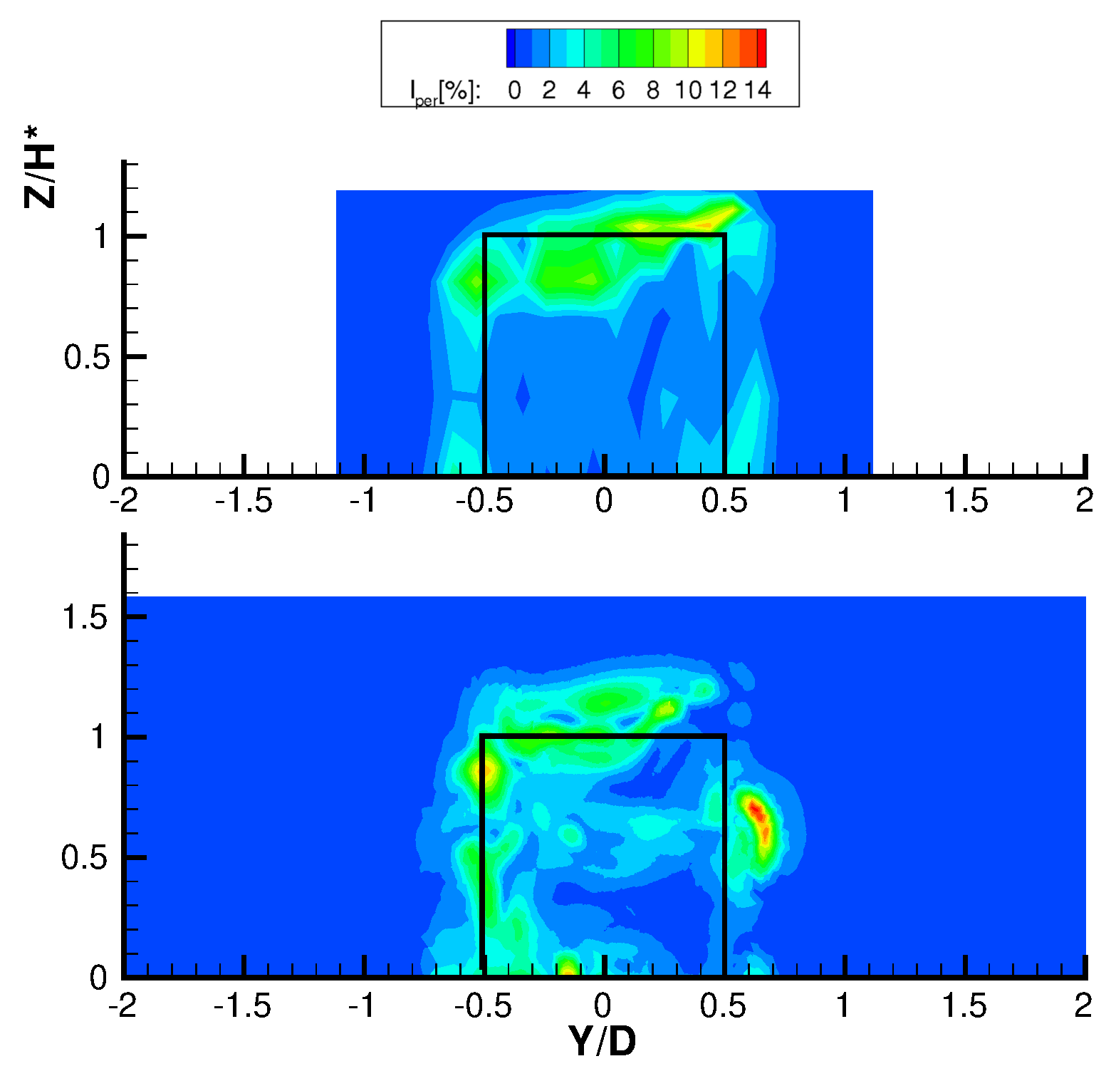
The inherent unsteadiness of VAWT operating principle has an implication on the wake, which undergoes both turbulence unsteadiness and a deterministic periodic unsteadiness locked on the blade revolution. To highlight the different unsteady contributions, in [16] a triple decomposition was introduced for VAWT wakes, which leads to the calculation of an intensity of periodic unsteadiness ($I_{PER}$). Figure 13 reports the distributions of periodic unsteadiness for TSR = 2.4, which is the more interesting configuration since very low periodic unsteadiness features the wake for TSR = 3.3. First focusing on $I_{PER}$, the wake exhibits the largest unsteadiness on the leeward (left) side, where the dynamic stall occurs (as seen in the computed flow field on the equatorial plane of Figure 6) and large-scale vortices are periodically shed in the wake flow. High periodic unsteadiness is also found at the tip, where the trailing vorticity undergoes periodic unsteadiness due to the blade motion. The simulation confirms all the observations made on the experimental configuration, even though it indicates a large periodic unsteadiness corresponding to the struts, not captured by the experiments due to the absence of a proper experimental resolution in this area. Examining the distribution of unresolved unsteadiness, the simulations confirm the highest turbulence intensity on the leeward side of the wake, even if the overall intensity is everywhere smaller, owing to the already discussed reasons.

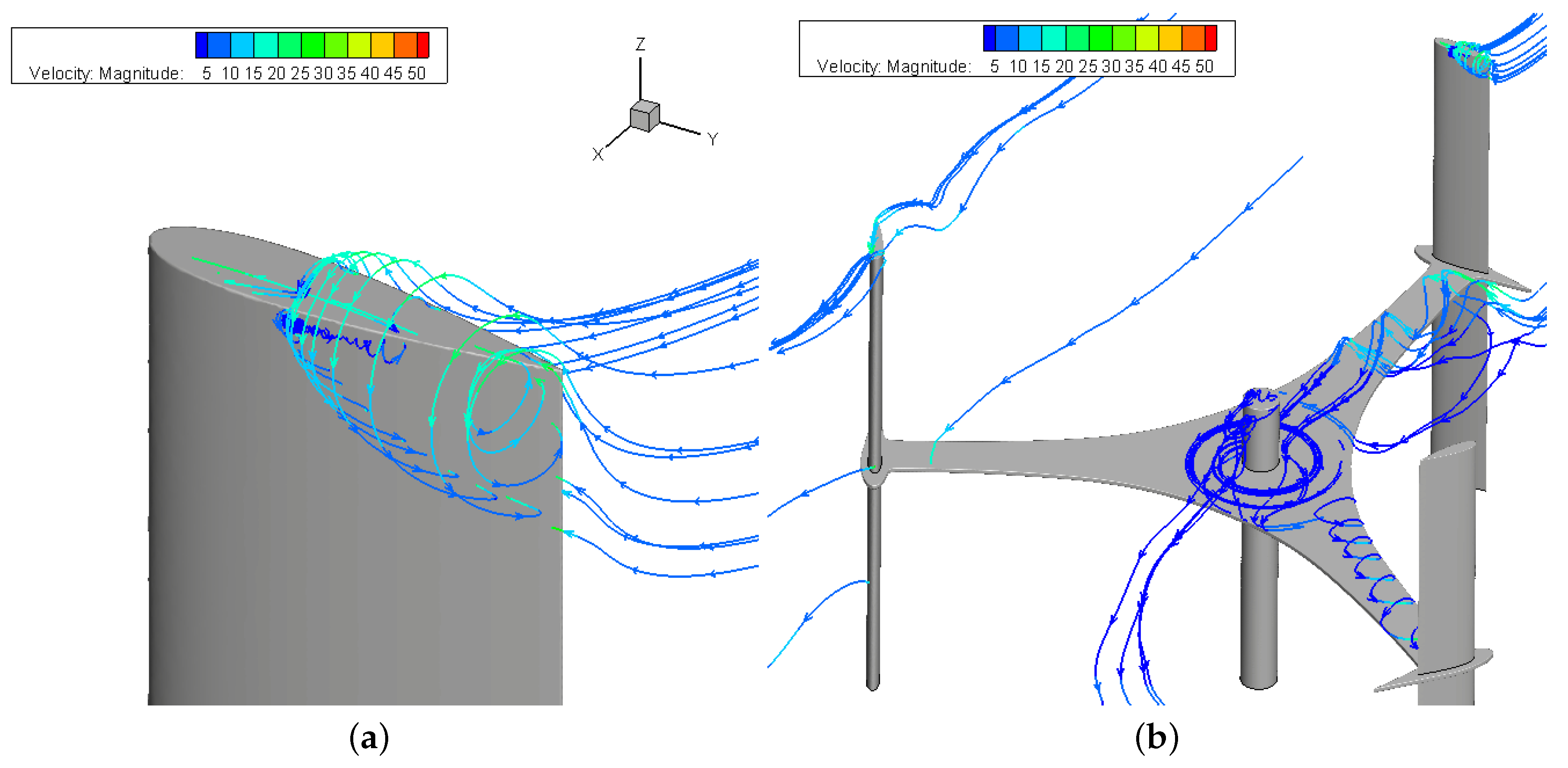
Evidence of the fully unsteady and three-dimensional character of the flow around the VAWT is given in Figure 14, where the complex tip and strut aerodynamics are shown. Notice the whirling flow near the struts and at the top of the shaft that contributes to reduce the extracted power, according to the velocity deficit previously described, due to interaction between the freestream flow and solid walls. Frame (b) of the same Figure shows another relevant feature of VAWTs, i.e., the dependence of the tip vortex on the local position of the blade during the rotation. The streamlines close to the two blade tips visible in Figure 14b show very different flow phenomena; in particular, a wide roll-up of streamlines occurs on the blade placed in the upwind part of the revolution (the one on the top-right part of the frame), similar to the one shown in frame (a). This is consistent with the blade position, as in the upwind part of the revolution both the high flow velocity and the high angle of attack contribute to generate high aerodynamic loading; this induces high work extraction but also high loading, and hence high trailing vorticity. Conversely, the blade operating in-between the leeward and downwind phases of the revolution (the one on the left side of Figure 14b) operates with a lower flow velocity (because of the work extraction in the upwind phase) and with a very high angle of attack, which exceeds the stall limit. As a result, the blade aerodynamic loading established on the blade is relatively low and, hence, the tip vortex is also much weaker with respect to the one in the upwind phase of the revolution. The variation of the tip vortex during the rotation results in a time-periodic evolution of the flow velocity downstream of the turbine in the tip region, thus providing a physical explanation of high $I_{PER}$ observed in both experiments and simulations at the tip border of the wake.

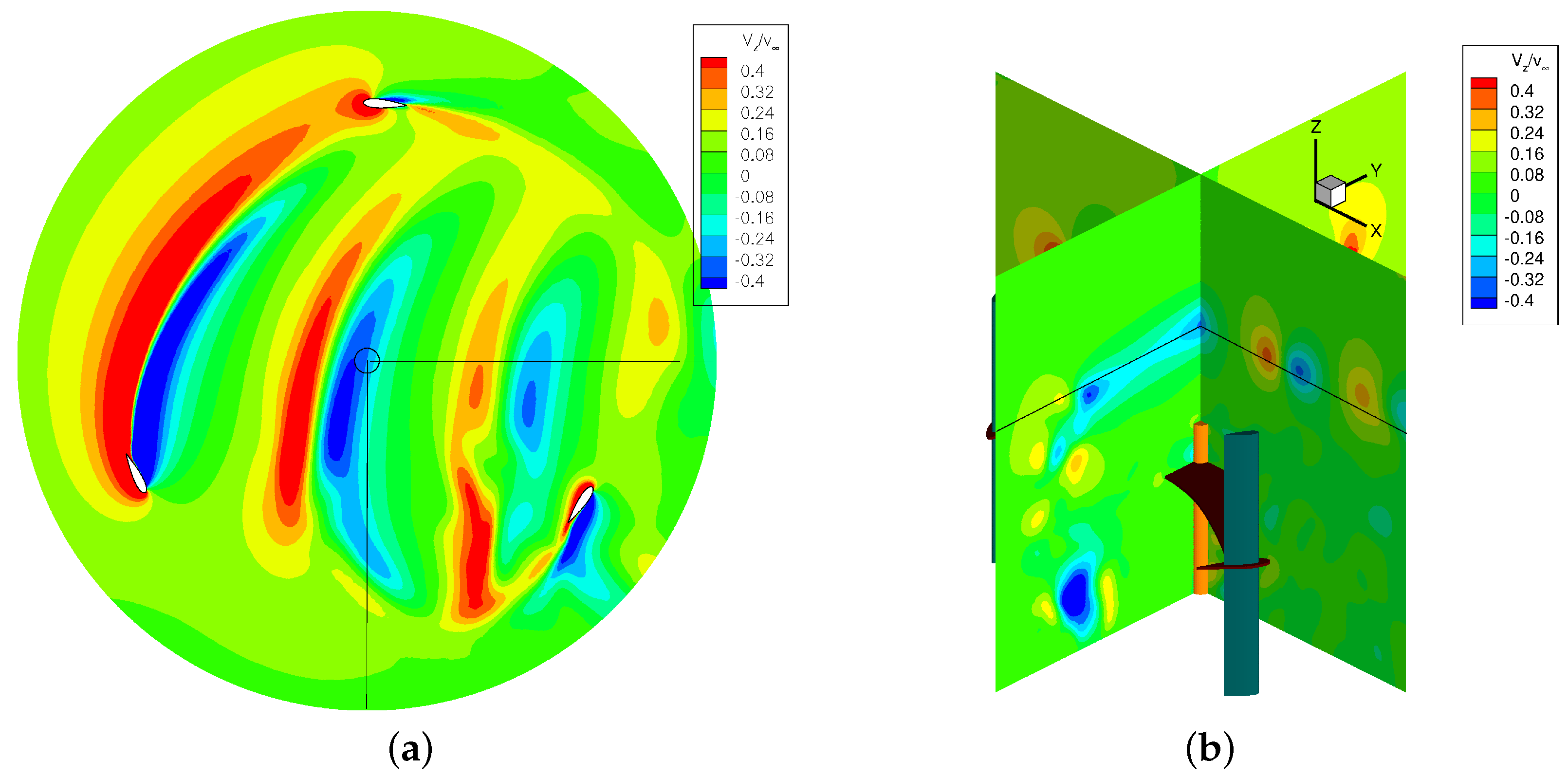
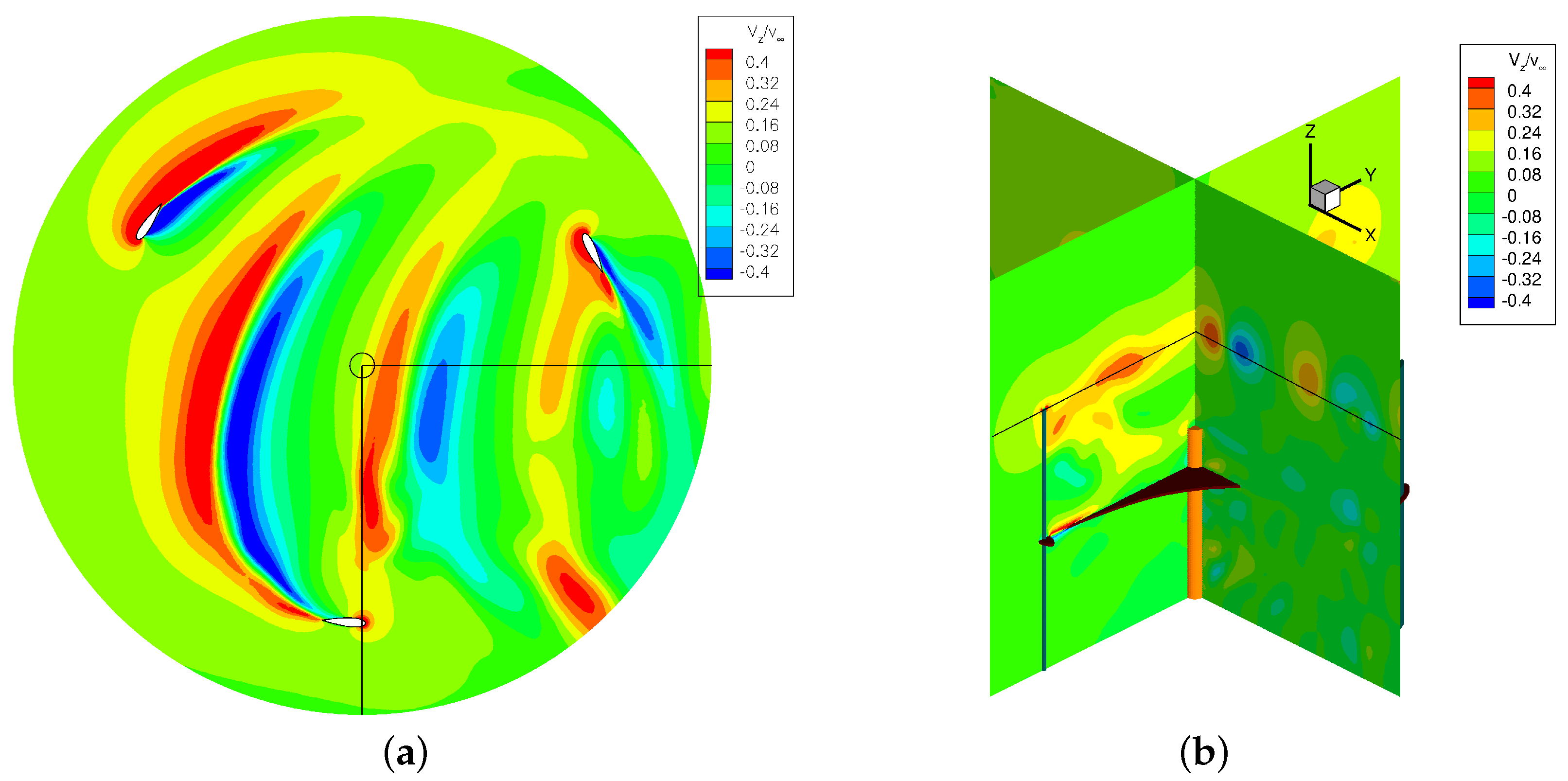
Finally, further illustration of the complex three-dimensional flow field characterizing the turbine is provided in Figure 15 and Figure 16 where snapshots of the non dimensional axial velocity are shown for two blade azimuthal positions, separated by half the rotor angular pitch. Secondary vortices are centered where isocontours are swiftly passing from negative to positive values and conversely. The left (a) part of the images refers to a plane close to the blade apex: tip vortices are clearly displayed and it is evident how their persistence through the turbine flow field is much greater than that shown by viscous wakes (see for example Figure 8). Note also that during both the blade advancing and retreating phases the tip vortex changes the direction of rotation: what will be seen in a time-averaged picture taken at a downstream x-constant plane depends therefore upon their relative initial strength and history. The sequence of travelling clockwise and counter-clockwise vortices is well visible on the semi-plane $y=0$ in the right (b) part of Figure 15 and Figure 16. On the semi-planes $x=0$ other vortical structures than the blade tip vortex can be detected. In Figure 15, there are vortices that arise from the tilting of the shed axial vorticity by means of the upward flow motion away from the symmetry plane, whereas Figure 16 shows how the strut boundary layers move radially outward under the influence of centrifugal forces and deflect in the axial direction when approaching the strut-blade junction. Evidence is thus given of the interaction between the flow and solid walls during the turbine revolution, with the flow rolling up over the airfoil surface and vortices developing along both blades and strut. These pictures give further qualitative indication of how the 3D effects related to finite blade length and presence of the strut may affect the turbine aerodynamics and performance.

6. Conclusions

This paper presented a computational study of the flow around a lift-driven H-shaped VAWT at two operating conditions: one for a tip speed ratio close to that of maximum power coefficient and another at a considerably higher tip speed ratio. The simulations benefit from a novel mathematical set-up that allows one to perform fully 3D simulations of the flow around the rotor and of the wake development with an industrially-relevant computational cost; an achievement still missing in the literature. The numerical predictions were assessed via a systematic comparison with experimental benchmark data, consisting of both performance and wake measurements carried out in the large-scale wind tunnel of the Politecnico di Milano. The quantitative comparison shows that the reliable simulation of the actual 3D and unsteady rotor aerodynamics of such class of machines is still a challenge, which might even require the use of different flow models in different operating conditions. The turbulence model, in particular, was found to be crucial to properly predict the onset of periodic separations on the blades and their consequences on both the tip vortex development and on the boundary layer generation on the struts. In the context of the $k-\omega$ SST turbulence model, the use of the low-Reynolds correction to introduce the effects of transition was proved to be accurate only at higher TSR, while the high-Reynolds (namely, fully turbulent) model resulted significantly more accurate at lower TSR condition. The proper selection of the turbulence model allowed limiting the difference between the measured and the predicted power coefficient to 0.025. In light of the model reliability, the detailed comparison between 2D and 3D simulations showed the impact of strut and tip effects on the overall torque exchanged between the flow and the rotor. In particular, the passive effects due to the three-dimensional flow features were found to affect mostly the active phase of the revolution, while having a limited impact in the downwind portion of revolution characterized by negative or null torque exchange; the analysis of the 3D flow field corroborates the quantitative findings with proper physical explanations.The flow models also allowed to achieve a very good prediction of the near-wake development, in terms of wake shape and velocity deficit. The reliability of the calculations and their potential for phenomenological analyses of the flow field make the present model suitable for application to other, more complex turbine operating conditions and architectures; future work will focus on both these subjects.