Article

Numerical Fatigue Analysis of a Prototype Francis Turbine Runner in Low-Load Operation †

Institute for Energy Systems and Thermodynamics/E302, TU Wien, Getreidemarkt 9/BA, 1060 Vienna, Austria
*
Author to whom correspondence should be addressed.
This paper is an extended version of our paper published in Proceedings of the European Turbomachinery Conference ETC13, Lausanne, Switzerland, 8–12 April 2019, Paper No. 123.
Int. J. Turbomach. Propuls. Power 2019, 4(3), 21; https://doi.org/10.3390/ijtpp4030021
Submission received: 30 April 2019 / Revised: 11 July 2019 / Accepted: 22 July 2019 / Published: 25 July 2019

Abstract

:
Depending on a dynamical energy market dominated by the influence of volatile energies, the operators of hydro-power plants are forced to extend the operating range of their hydraulic machines to stay competitive. High flexibility towards low-load, a rising number of start-ups and fast response times are required for better control of the electrical grid. The major downside of these operating regions is that pressure pulsations, which are induced by the means of flow phenomena, lead to higher fatigue damage regarding the runner. Therefore, site measurements in combination with numerical methods can be used to gain a deeper understanding of the runner lifetime. This paper presents a numerical approach to understand the critical operation zones and access fatigue damage, including steady state, unsteady and transient computational fluid dynamic (CFD) one-way coupled with a transient finite element method (FEM).

1. Introduction

In the past, many Francis turbines have operated near the rated point (RP) to provide base load supply. However, operators of hydro-power plants are currently facing a completely different energy market due to the increasing amount of renewable energies in use, such as solar and wind power [1]. Consequently, the prices on the spot market are continuously on a low level, contrary to the higher prices of control power. Therefore, operators of hydro-power plants are forced to extend their operating range to stay competitive in the market by ensuring grid stability. In Francis turbines, low-load, a high number of start-ups and flexible operation changes causing vortices and cavitation depending on operating conditions and specific speed, as it was shown by Escaler et al. [2]. These transient flow phenomena can be a reason for increased dynamical load and further for a decrease of the runner lifetime [3]. Consequently, fatigue analysis has become highly important for operators of hydro-power plants who wish to prevent cracks and expensive failure events. Especially in the case of medium head Francis turbines, the impact on fatigue life of transient events is significant [4].
Previously, detailed but expensive prototype site measurements, such as the one published by Dörfler et al. [5], were the only reliable source to gain information about the turbine behavior. However, over the last two decades, computational resources have increased immensely and the simulation approach has been continuously improved. A numerical lifetime investigation has already been published by Doujak et al. [6] and Coutu et al. [7] but still relies on measurements for validation. Therefore, the so-called fluid–structure interaction (FSI) plays a key role. In addition to a one-way coupling, a more complex two-way approach may be possible, which would lead to an increase of accuracy, especially if the deformations are significant [8]. However, based on computational resources and consuming time, several studies have shown that one-way coupling [9] is still appropriate even if the tendency to underestimate the stresses is slightly higher. Furthermore, the study by Eichhorn et al. [3] has shown that numerical analysis can predict runner stress with sufficient accuracy within stationary load points, even if unsteady flow is present. However, reproducing transient events—such as the load rejection by Jakobsen et al. [10] and Pavesi et al. [11] or the start-up simulated by Minakov et al. [12] and Nicolle et al. [13]—is still challenging. Especially in the case of a prototype machine, long simulation times and the complexity of the physics involved paired with a lack of validation cases leads to many difficulties. The accuracy of the dynamic stress prediction depends on the pressure fields and, therefore, mainly on the CFD modeling approach. Accordingly, advanced turbulence models—such as scale-adaptive-simulation (SAS), including suitable mesh refinement—are key to detecting vortex structures by the use of CFD simulations. With advanced CFD approaches and a refined mesh, the amplitudes of pressure pulsation tend to be smaller than the real ones [14]. Based on the experience gained by a previous research project [3,6,15,16], the authors performed detailed measurements on a prototype hydro-power plant to assess fatigue life and further validate a numerical simulation approach. The procedure, method and an analysis of the strain gauge measurement and an experimental fatigue assessment is already published in [17]. The setup of the measurement and a first analysis of the obtained data are presented in [18].
The aim of the work is to further develop the numerical approach for lifetime prediction of a prototype Francis turbine focusing on the critical low-load region. In contrast to previous publications, it also presents a way of including transients events in a numerical fatigue assessment. In order to validate the results, the simulations are compared to measurement data.

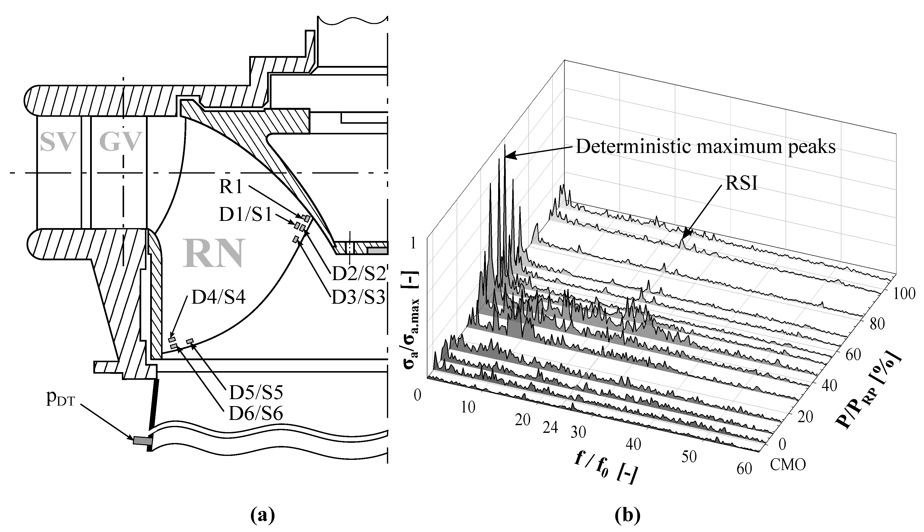
2. Prototype Site Measurements

To investigate critical operating points, site measurements on a medium head Francis turbine with a specific speed of n q 56 r e v m i n were performed. The main geometrical properties are summarized in Table 1.
Several operating points and transient events, such as start-up and condenser-mode-operation (CMO), were included in the measurement procedure. To investigate the behavior of the machine, numerous pressure transducers and vibration sensors have been installed. Regarding the following numerical investigations, the position of the static wall pressure measurement p D T in the draft tube near the runner is shown on the left-hand side of Figure 1. The piezo-resistive transducer is used for measurements in a range of 0–10 bar with a maximum measurement uncertainty of ± 0.2 % . The sample frequency is set at 3 kHz ensuring a sufficient range to capture expected pressure pulsation induced by flow phenomena [19]. The flow rate and thus also the mass flow was determined by the Winter Kennedy method, according to IEC 60041 standards [20], with a sample frequency of 10 Hz. Moreover, to obtain the dynamic stress, several uniaxial (D1–D6, S1–S6) and one multiaxial ( R 1 ) strain gauges have been applied on one runner blade at the pressure side (D) and suction side (S) close to the trailing edge, as shown in Figure 1a. On the right-hand side, Figure 1b shows the frequency spectrum of the uniaxial sensor D 2 , starting at the operating point with a power output of around 50 % of the rated power ( P R P ). In this region, a high peak appears in the low frequency regime. This peak corresponds to f / f 0 0.8 slightly beneath the rotational frequency f 0 .
Considering previous investigations of the Francis turbine off-design operation region, such as the one published by Escaler et al. [2], this indicates the occurrence of a draft tube vortex formation. However, sufficient unsteady CFD calculations are required to prove this estimation. Moreover, the harmonic peaks induced by the rotor–stator interaction between runner and guide vanes can also be seen. In contrast to a previous investigated high head machine [3], the impact of this phenomenon can be considered as very low compared to the peaks at low-load operation. Furthermore, a publication, including a brief description of the strain gauge measurement and the fatigue assessment based on it [17], revealed the most damaging operating point at 44 % · P R P .

3. CFD Analysis

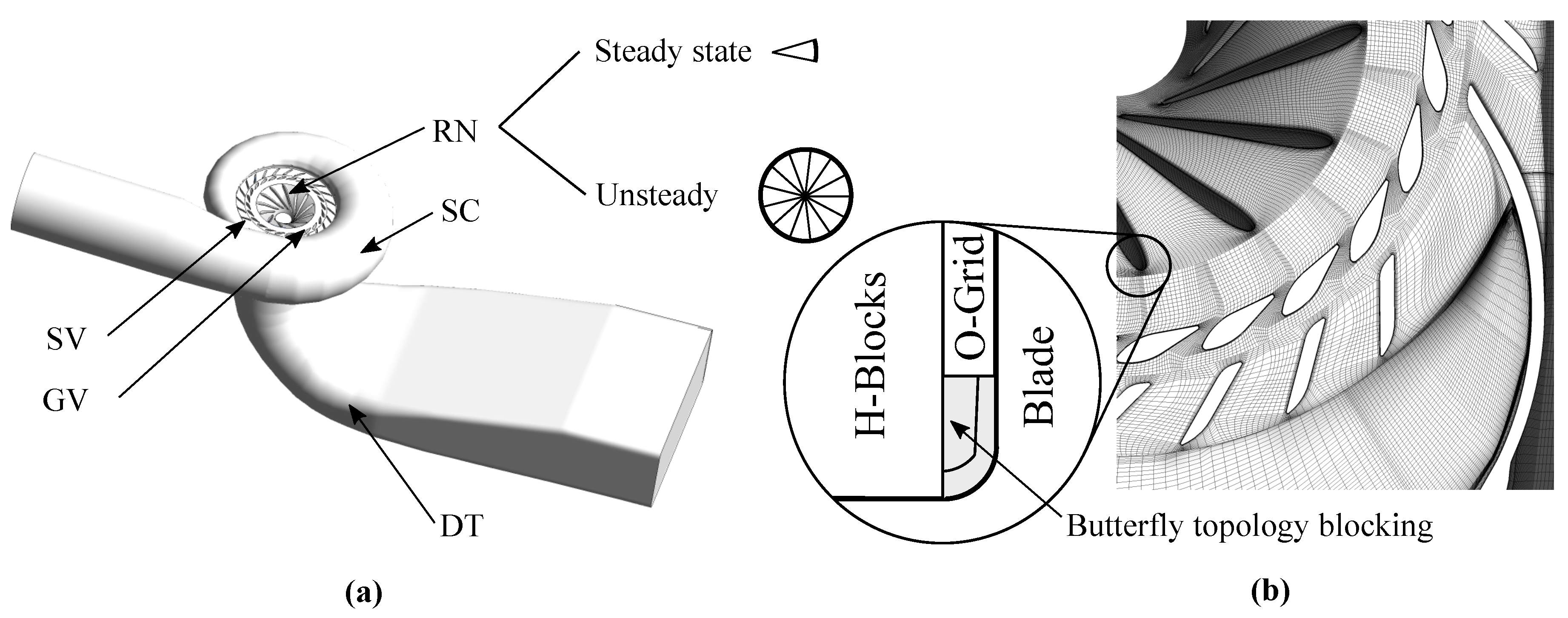
3.1. Discretization of the Prototype Francis Turbine

The CFD simulations are performed with the ANSYS CFX commercial software (Version 18.1 , ANSYS, Canonsburg, PA, USA) using Reynolds averaged (RANS) and further unsteady Reynolds averaged (URANS) Navier–Stokes equations (NSE). According to Figure 2a, a full model of the prototype machine is used for CFD calculations, including spiral casing (SC), stay vanes (SV), guide vanes (GV), runner (RN) and draft tube (DT). Due to the requirement of a high number of cells in the side-chamber, the leakage system was not included in the CFD-model. The particular domains, except RN, were discretized in multiblock full hexahedral grids using ANSYS ICEM 18.1 . In case of RN, NUMECA AUTOGRID5 (Version 12.2 , NUMECA, Brussels, Belgium) was used to deal with the highly curved blades. As shown on the right-hand side of Figure 2, a user-defined butterfly topology was created for the fillet mesh generation. Especially in terms of orthogonality, this ensures a significant better mesh quality for highly curved blades without using any major geometry simplifications. For the purpose of performing unsteady CFD simulations, besides a sector model, a full runner was modeled to avoid periodic boundary conditions. The entire mesh consists of about 6 m cells for steady state simulations, including one runner sector. The quality of the mesh is evaluated regarding minimum 3 × 3 determinate, angle and y + values. The exact number of cells and quality of the meshes are summarized in Table 2.
To estimate uncertainty due to discretization, a grid independence study according to the on Richardson extrapolation and the approach of Celik et al. [21] was performed. Therefore, based on the mesh described in Table 2, the grid size
h = 1 N C i = 0 N C Δ V i ( 1 3 )
is refined in three different stages (fine—1, medium—2, course—3) by constantly increasing and decreasing the number of cells by approximately one third. In Equation (1), N C describes the the total number of cells and Δ V i the volume of the i t h cell. Moreover, a constant resolution of the wall boundary layer according to 20 y m e a n + 120 was ensured, which can be considered as typical for numerical simulation of hydraulic turbines as summarized for example by Trivedi et al. [22]. The convergence study is verified by evaluating three different parameters Φ , which are the head H, the mechanical power P and the efficiency η . The extrapolated values
Φ e x t 21 = r 21 p C Φ 1 Φ 2 r 21 p C 1
for a normalized grid size h n = 0 , with p C the order of the accuracy and r the refinement factor for one mesh to another. The convergence behavior of the system can be assessed by the discriminating ratio
R = Φ 2 Φ 1 Φ 3 Φ 2 ,
which compares the three different meshes for one parameter. As a criterion for numerical uncertainties, the grid convergence index
G C I 21 = 1.25 · e a 21 r 21 p 1 ,
with the relative error e a 21 and a safety factor of 1.25 suggested by Celik et al. [21] amongst others.

3.2. CFD Setup

3.2.1. Steady CFD Setup

At first steady state, CFD calculations are done at the RP of the machine. This operating point is close to maximum power output and is used to perform a grid independence study on which further analyses can be based on. In terms of turbulence modeling, the shear stress transport (SST) model was used. The advection term is discretized by second-order upwinding while turbulence is approximated by a first-order scheme. As fluid, water at 20 C, treated as single-phase incompressible medium, is used. For coupling stationary interfaces, the General Grid Interface (GGI) was used. For the runner interfaces, a stage interface ensuring constant total pressure was implemented. At the inlet, the mass-flow according to the measurement was specified. Moreover, in order to accelerated simulation times, it is also consider to omit the SC. Therefore, a corresponding mass-flow distribution with an incidence angle is defined at the stay vane inlet. At the draft tube outlet, an average static pressure corresponding to a tailwater head Δ H 13 m is applied. To ensure sufficient convergence, 1000 iterations with a physical time step of 1 ω , which corresponds to one runner rotation, were done.

3.2.2. Unsteady CFD Setup

Another target of the investigation was to use numerical simulations for the purpose of finding evidence that vortices are causing high dynamical loads onto the runner blade. Therefore, the sector model was replaced by a full 360 runner and the draft tube mesh was particular refined near the inlet. The resulting grid consists of about 13 m cells and is based on the medium mesh (see Table 2). The boundary conditions at the SC inlet and DT outlet remain the same as for the steady analysis. The time step was set to a value corresponding to 1 of one runner rotation and the SAS-SST hybrid turbulence model is endorsed. The first order upwind scheme is used to interpolate the turbulence transport and a bounded central difference (CDS) scheme is applied to approximate the advection term. Moreover, a steady state simulation is used as an initial solution to improve and speed-up the convergence. Furthermore, a total amount of 15 runner rotations were simulated.

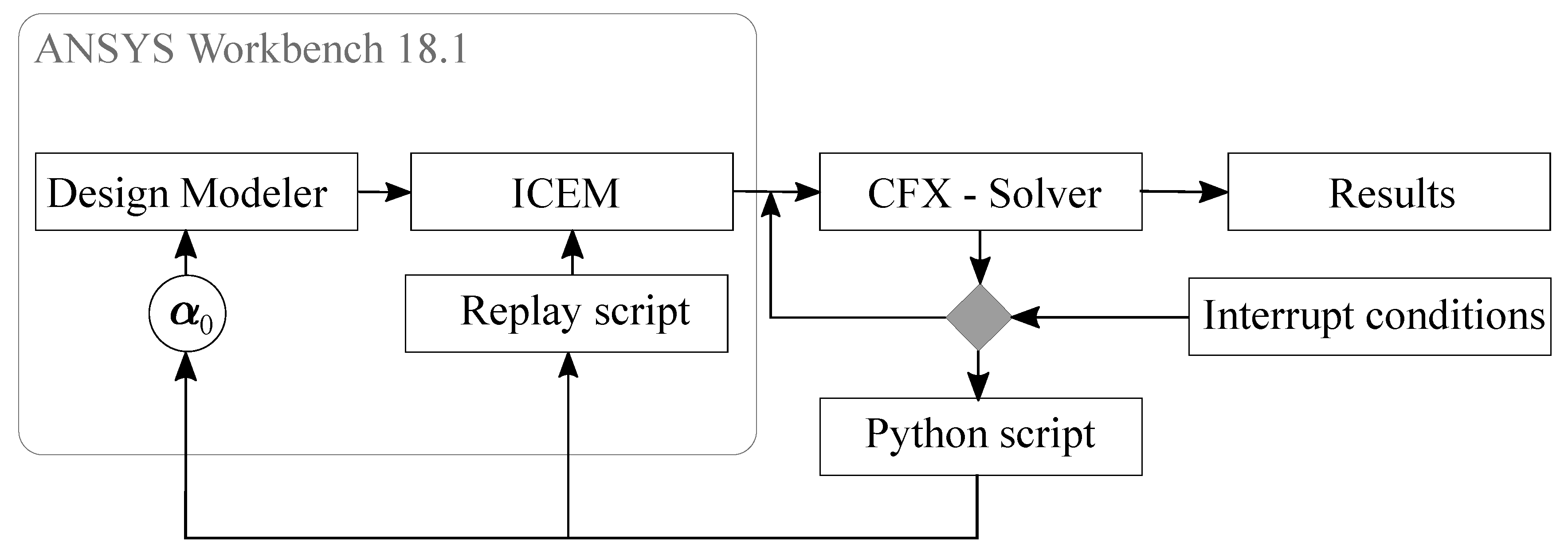
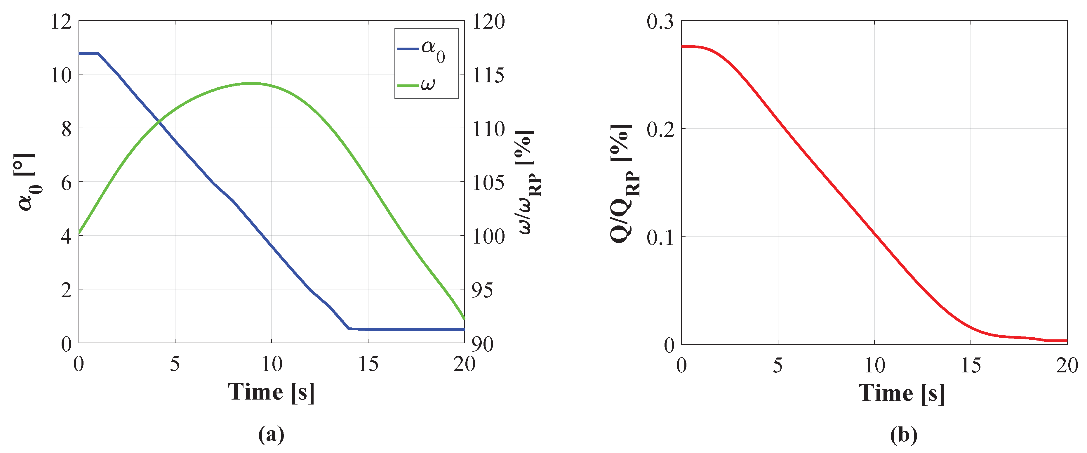
3.2.3. Transient CFD Setup

Based on the results of the strain gauge measurement [17], the huge influence of transient events on the fatigue life is proven. Most of those load cases are at least particular taking place at the low-load region, where, even at steady boundary conditions, unsteady pressure pulsations are occurring. The main challenge is to capture these unsteady pressure pulsations, while at the same time many runner rotations are required for a sufficient start-up or shut-down simulation. In contrast to the unsteady CFD-setup, in a steady load point, as shown in the previous section, one has to implement GV movement while simultaneously changing boundary conditions such as discharge and angular velocity. The moving parts can be realized by a combination of a displacement diffusion model and a sufficient remesh procedure. ANSYS CFX 18.1 can already deform meshes by solving the equation
( Γ d i s p δ ) = 0 ,
with Γ d i s p the mesh stiffness and δ the displacement. Additionally, the stiffness
Γ d i s p = ( Λ R e f Λ ) C S t i f f
can be controlled exponentially to determine which cells are absorbing the majority of the mesh motion. In this equation, Λ is the control volume size and C S t i f f the model exponent to control how fast the increase occurs. The exponential control parameter is increased from the default value C S t i f f . r e f = 2 to C S t i f f = 8 leading to much better mesh qualities during the motion. Therefore, longer simulation times without the requirement of remeshing are achieved.
For the purpose of ensuring a desirable mesh quality interruption, controls based on reliable parameters such as minimum cell angel and y + are implemented. After the mesh quality is unsuitable, a remesh procedure using Iron Python (which is supported by ANSYS WB 18.1 and ICEM 18.1 ) is triggered. After loading the results in the solver and interpolating the values, the simulation can proceed until another remesh is required. The approach shown in Figure 3 is script based and only has drawbacks at very small openings ( α 0 2 ), where a change of the blocking approach is usually advantageous.
To investigate the possibility of including this approach in fatigue analysis, a preliminary test case has been modeled. Therefore, a load rejection event starting at 20 % · P R P was used. The boundary conditions were again chosen according to the measurements (Figure 4a,b). Considering constant tailwater levels [18], a constant static pressure boundary conditions corresponding to Δ H 13.5 m was used at the outlet. Moreover, angular velocity and GV opening according to the available measurement data was integrated in the simulation model. Figure 4a illustrates the GV opening angle α 0 and the normalized rotational speed ω / ω R P of the runner. The measured discharge normalized by the discharge at the RP is depicted in Figure 4b.
To ensure a suitable representation of the event, a total amount of approximately 15,000 time steps is simulated. One time step corresponds to a runner rotation of 4 . The rest of the CFD setup was equal to the previously described unsteady case. A total amount of 13 remeshes are used, until the final position of 0.5 was reached. The majority of them are required at very small openings where the diffusion approach is not as efficient as at higher openings. Therefore, a manual generation of the meshes including a blocking adaption is necessary, although this can possibly be included in further versions of the remeshing procedure.

3.2.4. Vortex Identification Criteria

There are numerous criteria to identify vortical structures in turbulence because a mathematically unambiguous definition is hard to find. The most popular methods in fluid dynamics are based on the local velocity gradient. The introduction of threshold values leads to equivalent results of these methods [23]. One of these popular and widely used criteria is the λ 2 -criterion published by Jeong et al. [24]. The λ 2 -criterion is using the gradient of the NSE for incompressible planar flow and decomposes it into a symmetrical S ̲ and an unsymmetrical Ω ̲ part, as described in [23] for example. By neglecting the effects of unsteady irrational strain and viscosity from the obtained equation, the pressure Hessian can be written as
S ̲ 2 + Ω ̲ 2 = 1 ρ · p ,
with ρ the density and p the local pressure. Finally, a vortex is identified by using the eigenvalues λ of S ̲ 2 + Ω ̲ 2 and showing connected regions where λ 1 λ 2 λ 2 < 0 .

3.3. Results and Discussion of the CFD Analysis

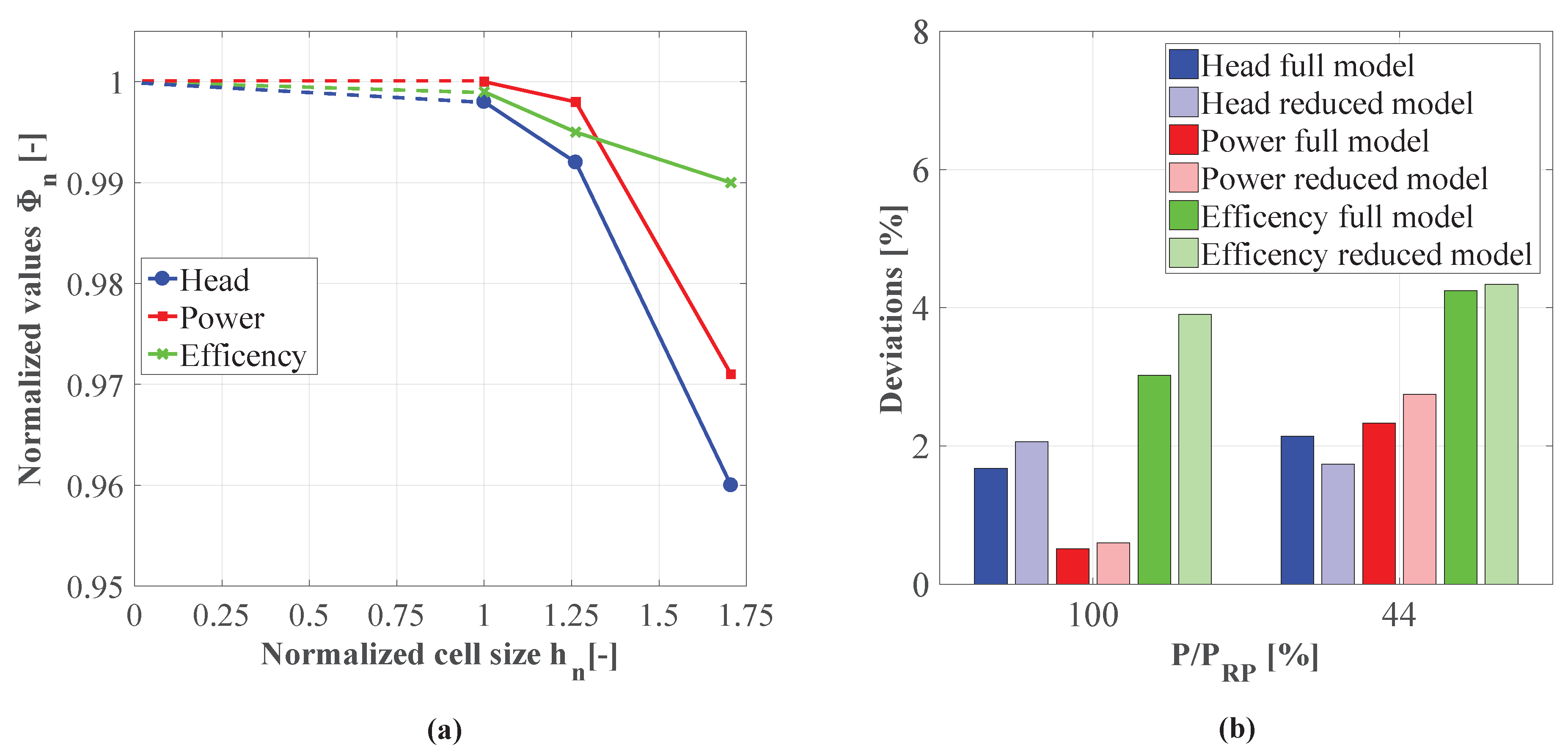
3.3.1. Steady State CFD Analysis and Grid Independence Study
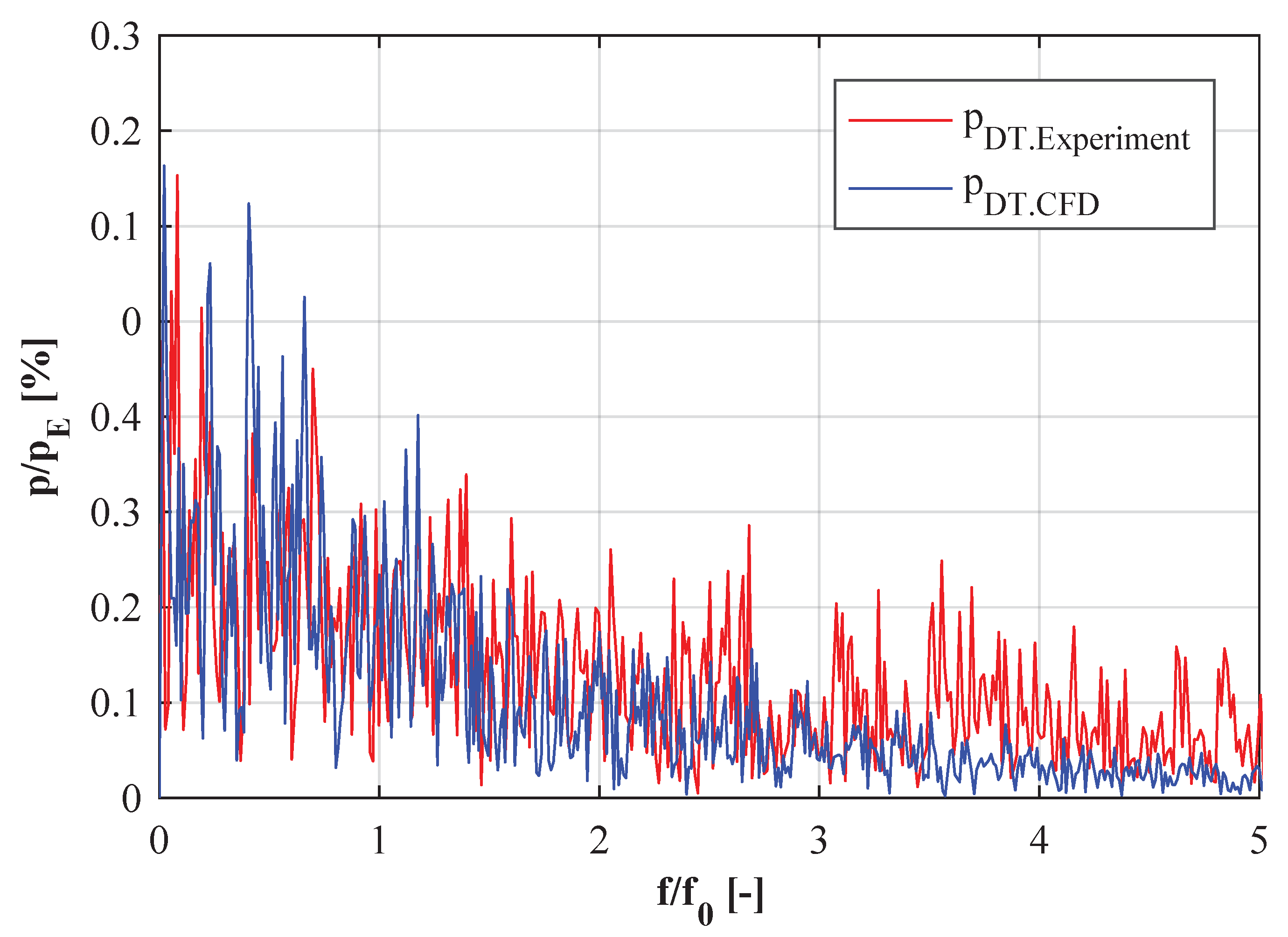
The left-hand side of Figure 5 shows the grid convergence for those parameters Φ normalized to the extrapolated values. The convergence behavior of the system can be assessed by the convergence or discriminating ratio, which compares the three different meshes for one parameter. According to a discriminating ratio of 0 < R < 1 , as suggested by Ali et al. [25] as well as Eça and Hoekstra [26], one can assume that monotonic convergence is present for all three parameters (Figure 5a).
The main discretionary uncertainty parameters are summarized in Table 3. As a criterion for numerical uncertainties, the grid convergence index (GCI) is suggested by Roache et al. [27] to be 1 % for the purpose of analyzing flow patterns. For the concerned case, the GCI is in a sufficient range between 0.03 % and 0.25 % referred to the medium mesh, which was chosen for further simulations.
Moreover, Figure 5b shows the deviation for H, P and η between experiment and CFD referred to measured values. Additionally, a case without the SC named as “Reduced model” was taken into account, to investigate the influence of the SC. One can see that the relative deviations for the global parameter show a good agreement. The values differ globally by less than 5 % and show a tendency to increase towards low-load. The influence of the SC on the global parameters can be considered as low. Therefore, this simplification could be used to reduce the amount of cells and further accelerate simulation times. However, for unsteady cases where flow phenomena can occur within the whole turbine, enlarging the inlet and outlet region is advantageous in terms of stability.

3.3.2. Unsteady CFD

The results of the unsteady CFD analysis at the critical load point ( 44 % · P R P ) are shown in Figure 6. As previously predicted, a noticeable draft tube vortex appears, which is displayed by the λ 2 -criterion in Figure 6a. The core of the vortex rope is rotating relatively uniformly, while, at the tail near the elbow, the structures fade away and collapse irregularly after emerging again. Moreover, on the right-hand side, the pressure distribution of the runner surface, normalized by the pressure corresponding to the circumferential velocity, referred to the outer diameter of runner outlet
p E = ρ · u 2 2 2 ,
is shown (Figure 6b). It is clearly evident that the occurrence of the vortex rope leads to particular high pressure magnitudes. Furthermore, the third picture on the left-hand side shows a plot of λ 2 -criterion superimposed by surface streamlines at section A-A, where the Sensor p D T is placed (Figure 6c). As one can see, the λ 2 -criterion indicates the appearance of vortex structure in the draft tube.
The fourth and last graph (Figure 6d) shows the frequency spectrum of the pressure fluctuations in the draft tube cone based on the measurement, as well as on the simulation. However, it can be difficult to obtain sufficient approximations of frequencies and amplitudes because of shift in periods and noise. Therefore, the Welch method [28] was applied splitting the measured signal into several Hanning windows considering 50 % overlap as suggested in [29]. The measured signal was then averaged and the deviations of the amplitude are marked by error bars. Further details about the method and its application in the field of experimental studies regarding hydraulic turbines can be found in [30]. Both signals show a similar behavior—a distinctive more or less harmonic peak at f / f 0 0.2 is clearly visible. Due to the unstable behavior of the draft tube vortex, the amplitude of the pressure signal varies over time by approximately 15 % in relation to its height. In Figure 6d, this is highlighted by error indicators. A sufficient agreement between both signals was reached, even if the simulated signal shows a tendency to underestimate the pressure fluctuations. The numerical model was optimized towards fatigue analysis. For a more accurate prediction of the vortex rope and accompanying smaller structures, one has to increase the number of cells in the draft tube.
Moreover, a higher simulation time and an adjustment of the time step would be advantageous to extract a signal with higher resolution.

3.3.3. Transient CFD

In this section, the results of the transient load rejection case are presented. Figure 7 shows a spectral analysis of the pressure fluctuations comparing experimental and numerical data to each other. Hence, the simulated pressure signal samples are not exactly equally spaced and an interpolation [31] was done with MATLAB (Version R2016, MathWorks, Natick, MA, USA), to ensure a sufficient application of the fast Fourier transform (FFT) algorithm. It can be seen that the overall pressure fluctuations were well predicted by the simulation. Within the low frequency range, the amplitudes show small differences, while, at higher frequencies, the simulated signal definitely underestimates the measured one.
By comparing Figure 7 with the results of the unsteady low-load case shown in Figure 6d, it can be concluded that the spectrum of the load rejection case is obviously more irregular. This is a result of the transient operation and very low openings, where the pressure pulsations are more or less stochastically distributed. In particular, at α 0 = 0.5 , the simulation tends to underestimate the pressure pulsations by a larger amount than at higher openings.
Figure 8 shows the flow behavior inside the runner at three different states of the closing process. On the left-hand side, the velocity field superimposed by streamlines describes the flow behavior inside the runner. On the contrary, the right-hand side shows regions where the pressure drops beneath the vapor pressure by means of iso-surfaces. From the beginning, the turbine has to deal with suboptimal flow conditions as load rejection was performed based on the 20 % · P R P operating point. Bad flow angels at the inlet, and an already huge circumferential component of the absolute velocity at the outlet, can lead to the appearance of separation and channel vortices as well as draft tube vortex formations. Figure 8a shows that a small channel vortex near the hub and close to the suction side is already present at the initial state. Additionally, a distinctive but unstable draft tube vortex spiting up into two tails is highlighted by iso-pressure surfaces (Figure 8b).
The maximum over-speed of 115 % is reached after approximately 9 s, as it can be seen in Figure 4a. In this state, the GV are already halfway closed and the flow situation inside the runner changed completely. The channel vortex on the suction side is still present, but there is also a pumping motion fueling the development of more distinctive vortex near pressure side, which can be seen in (Figure 8c). This flow behavior is quite similar to the one reported by Trivedi et al. [32]. The draft tube vortex formation is entirely vanished and there are just small vapor pressure regions moving away from the runner (Figure 8d).
Finally, Figure 8e,f shows the flow behavior at the end of the simulation, where the GV are almost closed. A strong pumping vortex on the suction side together with a very distinctive channel vortex are leading to an almost complete blockage of the entire runner. As a result of a discharge close to zero, there are no vortex structures or separation regions present in the draft tube.

4. FEM Analysis and Runner Fatigue

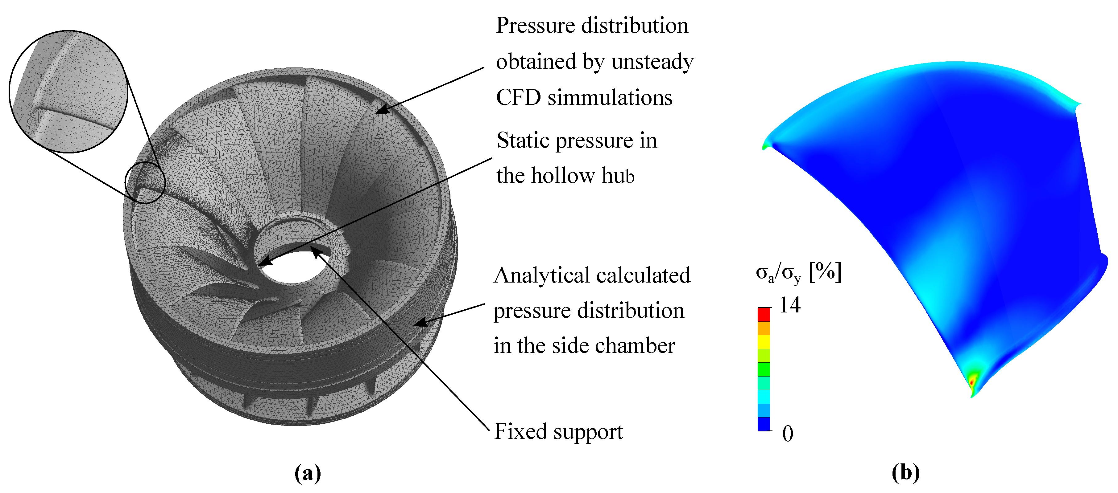
4.1. Transient FEM Simulations

To evaluate the influence of pressure fluctuations on the structure and fatigue life of the runner transient, FEM simulations by the use of ANSYS Mechanical 18.1 are performed. Therefore, a one-way coupling was used to apply the pressure fields onto the tetrahedral mesh of the runner. The FEM simulations were performed with a time step according to a runner rotation of 3 for the unsteady and 4 for the transient case. Critical and limiting factors in this regard were the computational time and resources. The structure damping is considered by the use of an equivalent Rayleigh damping. The left-hand side Figure 9a shows the setup including boundary conditions for a runner mesh of about 0.7 m nodes. Besides the pressure distribution on the runner blades, gravitational and rotational forces are considered. Moreover, an analytically calculated pressure distribution is used to model the pressure decrease by means of the labyrinth seals. The approach is already validated by the use of a model pump-turbine [33]. As suggested by Eichhorn et al. [3], amongst others, one runner blade was particularly refined near the hub and the shroud where the strain gauges were positioned. On the right-hand side, the dynamical stress σ a at one runner blade normalized by the yield strength σ y of the material is shown (Figure 9b). It can be seen that, at the displayed time step, the maximum appears near the location of S 2 , which corresponds well with the measured data [17].

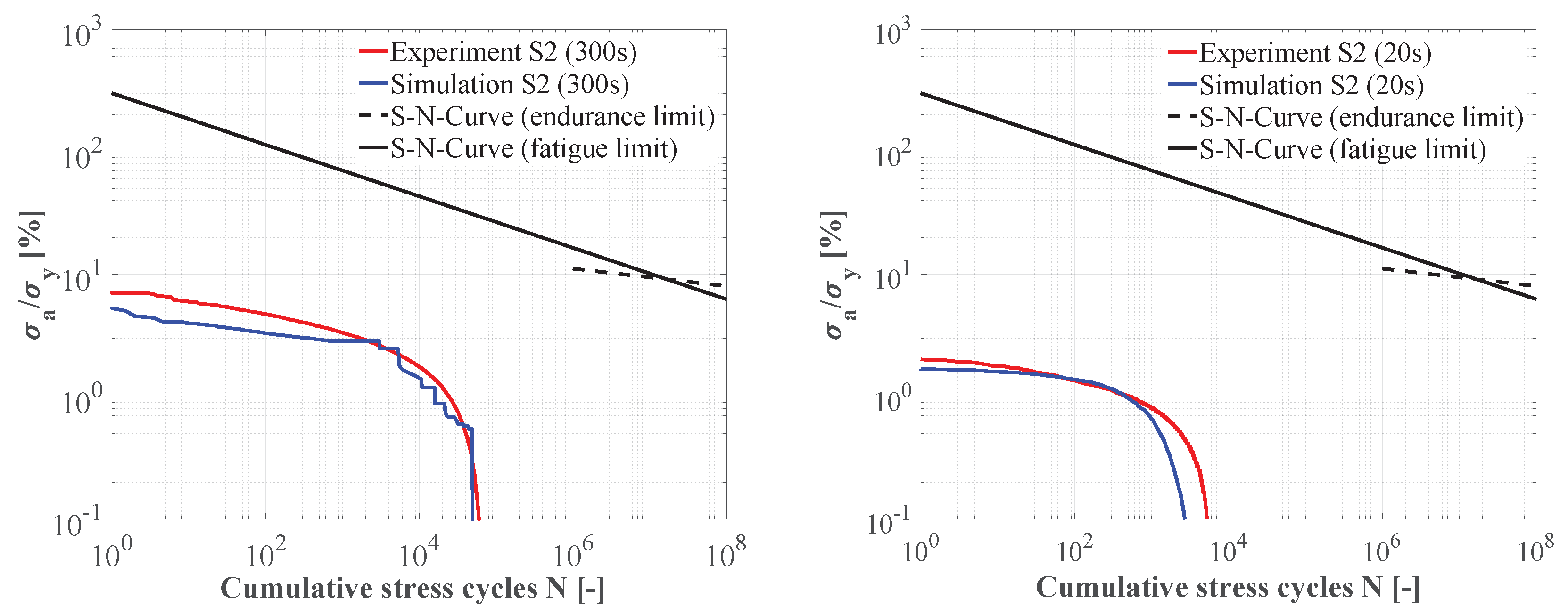
4.2. Fatigue Assessment

A fatigue assessment was done by evaluating the stress cycles by the use of a rainflow counting algorithm. Therefore, the stress signals at the strain gauge position of S 2 were calculated by averaging several nodes on that location, as shown in a previous publication by the authors [17].
To validate the simulation results, a comparison with the strain gauge data are presented. To approximate the time length scale of the computed signal, an extrapolation approach based on the extreme value theory published by Johannesson et al. [34] was used. To assess fatigue life, the stress cycles are compared to the S–N curve of the runner material for a 99 % survivability rate. The left-hand side Figure 10a shows the results for the critical low-load operation point ( 44 % · P R P ). Despite the underestimations of the pressure amplitudes, one can clearly point out that the results show an accurate agreement considering measurement uncertainties. Additionally, the results of the load rejection case were presented on the right-hand side (Figure 10b). In this respect again, the stress amplitudes underestimate the measurement in a smaller degree considering an extrapolation of the data was not needed. However, especially with regard to lower amplitudes, the load spectrum as a whole defers from that of the measurement. The rainflow curves of both cases are below the fatigue limit, even considering uncertainty.

5. Conclusions

The main target of the investigations was to evaluate the fatigue life of a prototype hydro-power plant by the use of numerical methods. Based on measurement data, an unsteady CFD simulation of the critical low-load operating point at 44 % · P R P was performed. A significant frequency of about 0.8 · f 0 in the rotating system and equal to 0.2 · f 0 in the stationary frame corresponding to the measurement data of strain gauges and pressure transducers was found. The reason for this is the appearance of a draft tube vortex structure, which leads to strong pressure pulsation. Moreover, an approach to simulate transient events was presented and tested on a load rejection case. The obtained pressure fields were used to perform transient FEM calculations to evaluate the load on the Francis turbine runner. In the last step, these stress amplitudes were validated by means of strain gauge measurements and further compared with the S–N-curve to assess the fatigue life of the runner. An appropriate agreement between the measurement data and the simulation results, which tend to underestimate the real values, was revealed. However, considering two-phase flow and using a two-way FSI coupling would most likely result in an improvement of the simulated results. Furthermore, in case of the transient load rejection case, the influence of stochastic distributed load at small GV openings still requires a huge amount of research. Moreover, for a transient simulation approach that does not depend on measurements, the implementation of a 1 D -Code is suggested. Another suggestion regarding the further development of the transient simulation would be an examination of the influence of the boundary conditions. It would also be advantageous to further investigate the applicability of the presented grid convergence approach on transient simulations. For a valuable lifetime prediction based on numerical or experimental investigations, the S–N curve as a key element still remains as an uncertainty. Consequently, it is recommended that more complex approaches considering low-cycle-fatigue and crack grow rates should be considered in the future.

Author Contributions

Conceptualization, J.U. and E.D.; methodology, J.U.; software, J.U.; validation, J.U.; investigation, J.U., E.D. and C.B.; resources, C.B., E.D. and J.U.; writing—original draft preparation, J.U.; writing—review and editing, E.D. and C.B.; visualization, J.U.; supervision, C.B.; project administration, E.D. and C.B.; funding acquisition, E.D. and J.U.

Funding

This work was funded by the FFG—Austrian Research Promotion Agency (BRIDGE, No. 861560) and the associated research partners Brüel & Kjær Vibro GmbH and Voralberger Illwerke AG. The APC was funded by the Euroturbo Association.

Acknowledgments

The authors would like to thank the project partners Brüel & Kjaer Vibro GmbH and Voralberger Illwerke AG for their contribution in the course of the research project. The computational results presented have been partly carried out by using the Vienna Scientific Cluster (VSC3).

Conflicts of Interest

The authors declare no conflict of interest. The founding sponsors had no role in the design of the study; in the collection, analyses, or interpretation of data; in the writing of the manuscript, and in the decision to publish the results.

Abbreviations

The following abbreviations are used in this manuscript:
Acronyms
CDSCentral deference scheme
CFDComputational fluid dynamics
CMOCondenser-mode-operation
DPressure side
DTDraft tube
GGIGeneral grid interface
FEMFinite element method
FFTFast Fourier transform
FSIFluid–structure interaction
GVGuide vanes
NSENavier–Stokes equations
RANSReynolds averaged NSE
R1T-rosette
RNRunner
RPRated point
RSIRotor-stator interaction
SSuction side
SASScale adaptive simulation
SCSpiral casing
SSTShear stress transport
SVStay vanes
URANSUnsteady RANS
Greek Symbols
α 0 Guide vane opening, [ ]
Γ d i s p Mess stiffness, [-]
Δ H Tailwater head, [m]
Δ V i Volume of the i t h cell, [ m 3 ]
δ Mesh displacement, [m]
η Efficiency, [-]
Λ Control volume, [ m 3 ]
λ Eigenvalues, [-]
Nabla operator, [-]
ρ Water density, [ k g m 3 ]
σ a Stress amplitude, [ N m 2 ]
σ y Yield strength, [ N m 2 ]
Φ n Normalized Parameters, [-]
Ω ̲ Unsymmetrical part of the NSE, [-]
ω Angular velocity, [ r a d s ]
Latin Symbols
C S t i f f Stiffness coefficient, [-]
D 1 . a Outer diameter (RN Inlet), [m]
e a Relative error, [-]
fFrequency, [ H z ]
f 0 Rotational Frequency, [ H z ]
G C I Grid convergence index, [-]
HHead, [m]
hCell size, [m]
h n Normalized cell size, [-]
N C Number of cells, [-]
n q Specific speed, [ r e v m i n ]
PPower, [ M W ]
pPressure, [ b a r ]
p C Order of accuracy, [-]
p E Dynamic pressure (RN outlet), [ b a r ]
QDischarge, [ m 3 / s ]
RConvergence Ratio, [-]
rRefinement factor, [-]
S ̲ Symmetrical part of the NSE, [-]
u 2 Circumferential velocity (RN outlet), [ m s ]
y + Absolute wall distance, [-]

References

  1. Balsalobre-Lorente, D.; Shahbaz, M.; Roubaud, D.; Farhani, S. How economic growth, renewable electricity and natural resources contribute to CO2 emissions? Energy Policy 2018, 113, 356–367. [Google Scholar] [CrossRef] [Green Version]
  2. Escaler, X.; Egusquiza, E.; Farhat, M.; Avellan, F.; Coussirat, M. Detection of cavitation in hydraulic turbines. Mech. Syst. Signal Process. 2006, 20, 983–1007. [Google Scholar] [CrossRef] [Green Version]
  3. Eichhorn, M.; Taruffi, A.; Bauer, C. Expected load spectra of prototype Francis turbines in low-load operation using numerical simulations and site measurements. J. Phys. 2017, 813, 012052. [Google Scholar] [CrossRef] [Green Version]
  4. Seidel, U.; Mende, C.; Hübner, B.; Weber, W.; Otto, A. Dynamic loads in Francis runners and their impact on fatigue life. In Proceedings of the IOP Conference Series: Earth and Environmental Science, Montreal, QC, Canada, 22–26 September 2014; Volume 22, p. 032054. [Google Scholar]
  5. Dörfler, P.; Bloch, R.; Mayr, W.; Hasler, O. Vibration tests on a high-head (740 m) Francis turbine: Field test results from Hausling. In Proceedings of the IAHR 14th Symposium on Hydraulic Machinery and Systems, Section for Hydraulic Machinery, Trondheim, Norway, 20–23 June 1988; Desbaillets, J., Ed.; TAPIR Publ: Trondheim, Norway, 1988; pp. 241–252. [Google Scholar]
  6. Doujak, E.; Eichhorn, M. An Approach to Evaluate the Lifetime of a High Head Francis runner. In Proceedings of the 16th International Symposium on Transport Phenomena and Dynamics of Rotating Machinery, Honolulu, HI, USA, 10–15 April 2016. [Google Scholar]
  7. Coutu, A.; Chamberland-Lauzon, J. The impact of flexible operation on Francis runners. Int. J. Hydropower Dams 2015, 22, 90–93. [Google Scholar]
  8. Benra, F.K.; Dohmen, H.J.; Pei, J.; Schuster, S.; Wan, B. A comparison of one-way and two-way coupling methods for numerical analysis of fluid–structure interactions. J. Appl. Math. 2011, 2011, 853560. [Google Scholar] [CrossRef]
  9. Huang, X.; Oram, C.; Sick, M. Static and dynamic stress analyses of the prototype high head Francis runner based on site measurement. In Proceedings of the IOP Conference Series: Earth and Environmental Science, Montreal, QC, Canada, 22–26 September 2014; IOP Publishing: Bristol, UK, 2014; Volume 22, p. 032052. [Google Scholar]
  10. Jakobsen, K.R.G.; Holst, M.A. CFD simulations of transient load change on a high head Francis turbine. J. Phys. 2017, 782, 012002. [Google Scholar] [CrossRef] [Green Version]
  11. Pavesi, G.; Cavazzini, G.; Ardizzon, G. Numerical simulation of a pump–turbine transient load following process in pump mode. J. Fluids Eng. 2018, 140, 021114. [Google Scholar] [CrossRef]
  12. Minakov, A.; Sentyabov, A.; Platonov, D. Numerical investigation of flow structure and pressure pulsation in the Francis-99 turbine during startup. J. Phys. 2017, 82, 012004. [Google Scholar] [CrossRef]
  13. Nicolle, J.; Giroux, A.; Morissette, J. CFD configurations for hydraulic turbine startup. In Proceedings of the IOP Conference Series: Earth and Environmental Science, Montreal, QC, Canada, 22–26 September 2014; IOP Publishing: Bristol, UK, 2014; Volume 22, p. 032021. [Google Scholar]
  14. Jošt, D.; Škerlavaj, A.; Morgut, M.; Mežnar, P.; Nobile, E. Numerical simulation of flow in a high head Francis turbine with prediction of efficiency, rotor stator interaction and vortex structures in the draft tube. J. Phys. 2015, 579, 012006. [Google Scholar] [CrossRef]
  15. Eichhorn, M.; Doujak, E. Impact of different operating conditions on the dynamic excitation of a high head francis turbine. In Proceedings of the ASME 2016 International Mechanical Engineering Congress and Exposition, Phoenix, AZ, USA, 11–17 November 2016; American Society of Mechanical Engineers: New York, NY, USA, 2016; p. V04AT05A035. [Google Scholar]
  16. Unterluggauer, J.; Eichhorn, M.; Doujak, E. Fatigue analysis of Francis turbines with different sepcific speeds using site measurements. In Proceedings of the 19th International Seminar on Hydropower Plants, Vienna, Austria, 9–11 November 2016; Technische Universität Wien, Ed.; Eigenverlag: Wien, Austria, 2016. [Google Scholar]
  17. Unterluggauer, J.; Doujak, E.; Bauer, C. Fatigue analysis of a prototype Francis turbine based on strain gauge measurements. In Proceedings of the 20th International Seminar on Hydropower Plants, Vienna, Austria, 14–16 November 2018; Technische Universität Wien, Ed.; Eigenverlag: Wien, Austria, 2018. [Google Scholar]
  18. Mühlbacher, K. Measurement Data Analysis of a Prototype Francis Turbine Site Measurement. Master’s Thesis, TU Wien, Wien, Austria, 2019. [Google Scholar]
  19. Dörfler, P.; Sick, M.; Coutu, A. Flow-Induced Pulsation and Vibration in Hydroelectric Machinery: Engineer’s Guidebook for Planning, Design and Troubleshooting; Springer Science & Business Media: Berlin, Germany, 2012. [Google Scholar]
  20. International Electrotechnical Commission. Field Acceptance Tests to Determine the Hydraulic Performance of Hydraulic Turbines, Storage Pumps and Pump-Turbines: IEC60041—1991.0; International Electrotechnical Commission: Geneva, Switzerland, 1991. [Google Scholar]
  21. Celik, B.; Ghia, U.; Roache, P.; Freitas, C.; Coleman, H.; Raad, P. Procedure for Estimation and Reporting of Uncertainty Due to Discretization in CFD Applications. J. Fluids Eng. 2008, 130, 78001. [Google Scholar] [CrossRef] [Green Version]
  22. Trivedi, C.; Cervantes, M.J.; Gandhi, B.K.; Dahlhaug, O.G. Experimental and numerical studies for a high head Francis turbine at several operating points. J. Fluids Eng. 2013, 135, 111102. [Google Scholar] [CrossRef]
  23. Chen, Q.; Zhong, Q.; Qi, M.; Wang, X. Comparison of vortex identification criteria for planar velocity fields in wall turbulence. Phys. Fluids 2015, 27, 085101. [Google Scholar] [CrossRef]
  24. Jeong, J.; Hussain, F. On the identification of a vortex. J. Fluid Mech. 1995, 285, 69–94. [Google Scholar] [CrossRef]
  25. Ali, M.S.M.; Doolan, C.J.; Wheatley, V. Grid convergence study for a two-dimensional simulation of flow around a square cylinder at a low Reynolds number. In Proceedings of the Seventh International Conference on CFD in The Minerals and Process Industries, Melbourne, Australia, 9–11 December 2009; pp. 1–6. [Google Scholar]
  26. Eça, L.; Hoekstra, M. A procedure for the estimation of the numerical uncertainty of CFD calculations based on grid refinement studies. J. Comput. Phys. 2014, 262, 104–130. [Google Scholar] [CrossRef]
  27. Roache, P.J. Quantification of uncertainty in computational fluid dynamics. Annu. Rev. Fluid Mech. 1997, 29, 123–160. [Google Scholar] [CrossRef]
  28. Welch, P. The use of fast Fourier transform for the estimation of power spectra: a method based on time averaging over short, modified periodograms. IEEE Trans. Audio Electroacoust. 1967, 15, 70–73. [Google Scholar] [CrossRef]
  29. Trethewey, M. Window and overlap processing effects on power estimates from spectra. Mech. Syst. Signal Process. 2000, 14, 267–278. [Google Scholar] [CrossRef]
  30. Vekve, T. An Experimental Investigation of Draft Tube Flow. Ph.D. Thesis, Norvegian University of Science and Technology, Trondheim, Norway, 2004. [Google Scholar]
  31. Akima, H. A new method of interpolation and smooth curve fitting based on local procedures. J. ACM 1970, 17, 589–602. [Google Scholar] [CrossRef]
  32. Trivedi, C.; Cervantes, M.; Gandhi, B. Investigation of a high head Francis turbine at runaway operating conditions. Energies 2016, 9, 149. [Google Scholar] [CrossRef]
  33. Maly, A.; Eichhorn, M.; Bauer, C. Experimental investigation of transient pressure effects in the side chambers of a reversible pump turbine model. In Proceedings of the 19th International Seminar on Hydropower Plants, Vienna, Austria, 9–11 November 2016; Technische Universität Wien, Ed.; Eigenverlag: Wien, Austria, 2016; pp. 675–684. [Google Scholar]
  34. Johannesson, P. Extrapolation of load histories and spectra. Fatigue Fract. Eng. Mater. Struct. 2006, 29, 209–217. [Google Scholar] [CrossRef] [Green Version]
Figure 1. (a) meridional contour of the considered Francis turbine including strain gauge position and (b) waterfall chart of the sensor D2.
Ijtpp 04 00021 g001
Figure 2. Discretization of the prototype hydro-power plant, (a) domains and (b) mesh.
Ijtpp 04 00021 g002
Figure 3. Remeshing procedure.
Ijtpp 04 00021 g003
Figure 4. (a) measured values of the GV opening and angular velocity during load rejection and (b) discharge obtained by the Winter Kennedy method.
Ijtpp 04 00021 g004
Figure 5. (a) Grid independence study and (b) comparison between measurements and CFD.
Ijtpp 04 00021 g005
Figure 6. Draft tube vortex structure highlighted by (a) λ 2 -criterion including (b) the pressure distribution of the runner and (c) the λ 2 -criterion used at the 2D plane at section A-A as well as (d) a compartment of simulated and measured pressure fluctuations ( 44 % · P R P ).
Ijtpp 04 00021 g006
Figure 7. Compartment of simulation and experiment by means of pressure pulsations.
Ijtpp 04 00021 g007
Figure 8. Flow field at the initial state (a) in the runner channel and (b) vortex structures in the draft tube. Flow field after 9 s (c) in the runner channel and (d) vortex structures in the draft tube. Flow field after 20 s (e) in the runner channel and (f) vortex structures in the draft tube.
Ijtpp 04 00021 g008
Figure 9. (a) setup and (b) results of the transient FEM simulation in the critical load region ( 44 % · P R P ).
Ijtpp 04 00021 g009
Figure 10. Load spectra of the measured and computed stresses for (a) the unsteady case at 44 % · P R P and (b) the transient load rejection case.
Ijtpp 04 00021 g010
Table 1. Main geometrical properties of the turbine.
R u n n e r d i a m e t e r D 1 . a [m]2
N u m b e r o f s t a y v a n e s [-]23
N u m b e r o f g u i d e v a n e s [-]24
N u m b e r o f r u n n e r b l a d e s [-]13
Table 2. Size and quality of the medium mesh.
DomainSCSVGVRNDT
N u m b e r o f c e l l s [m] 1.662 1.311 1.797 0.465 0.756 5.991
M i n i m u m d e t e r m i n a n t [-] 0.2 0.28 0.6 0.22 0.4 0.2
M i n i m u m a n g l e [ ] 10.3 24.9 33 15.8 27 10.3
y R P . m e a n + [-] 60.2 24.9 56.25 23.6 22.2 37.5
Table 3. Discretization uncertainties.
ParametersHeadEfficiencyPower
D i s c r i m i n a t i n g r a t i o R [-] 0.18 0.78 0.0687
R e l a t i v e e r r o r e a 21 [-] 0.58 0.4 0.18
E x t r a p o l a t e d r e l a t i v e e r r o r e e x t 21 [-] 0.2 0.06 0.02
G r i d c o n v e r g e n c e i n d e x G C I 21 [-] 0.25 0.08 0.03

