Flutter Analysis of a Transonic Steam Turbine Blade with Frequency and Time-Domain Solvers †

Abstract
:1. Introduction
2. Numerical Methods
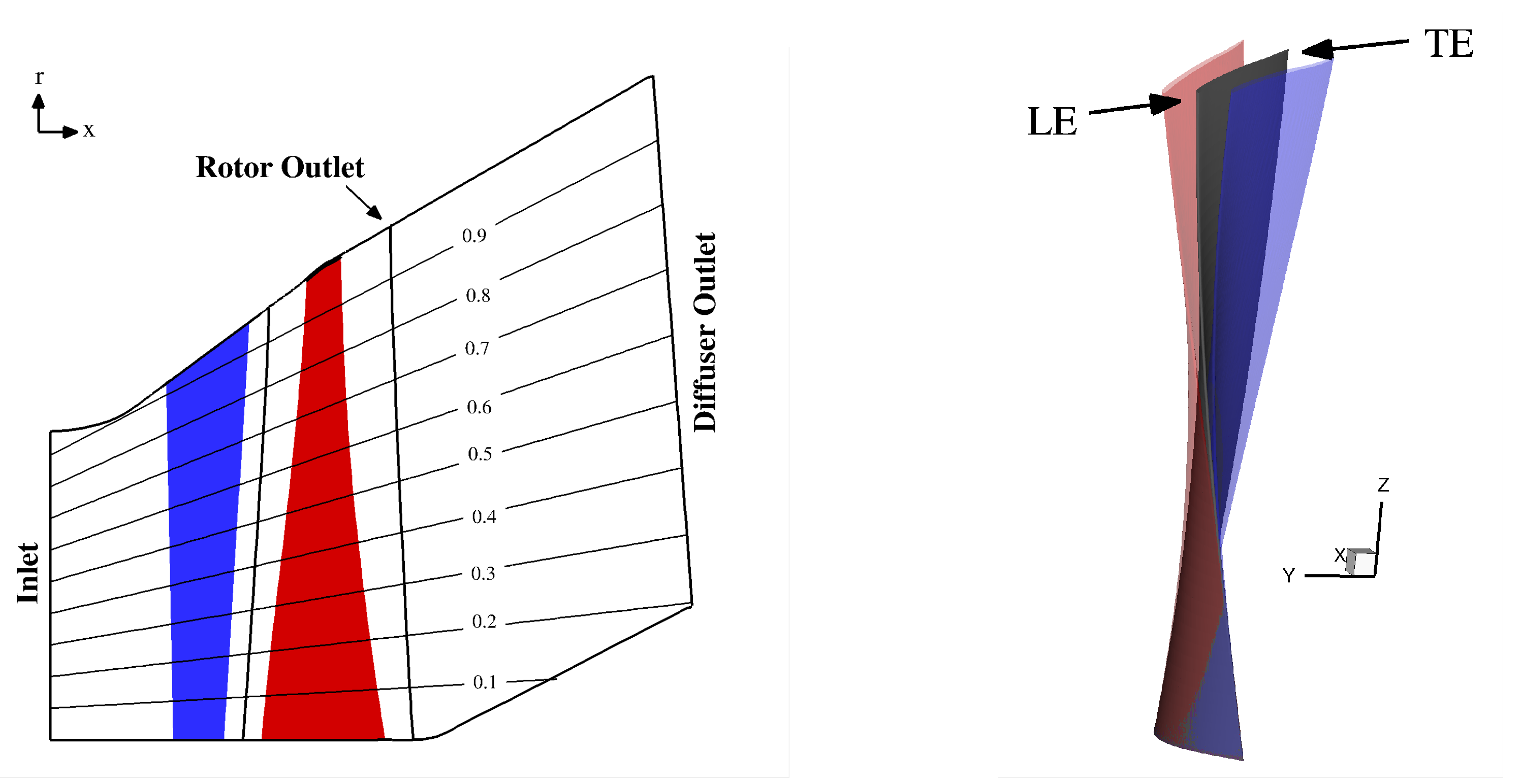
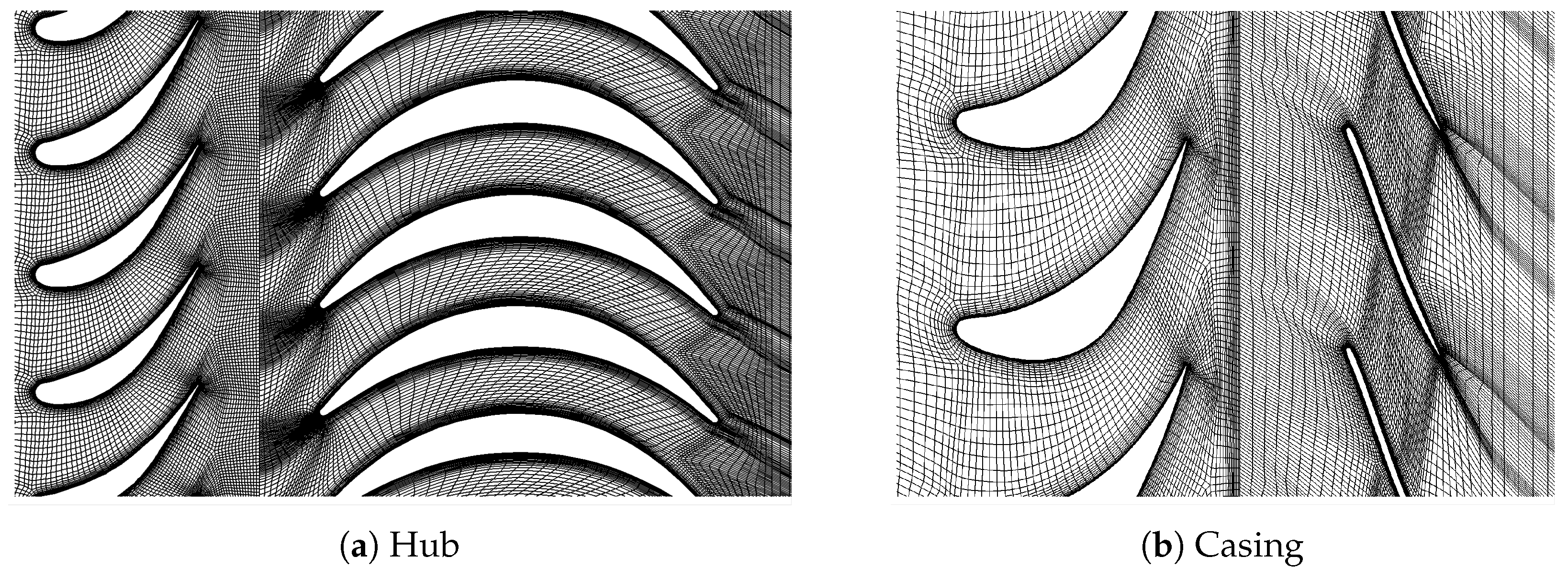
3. Test Case
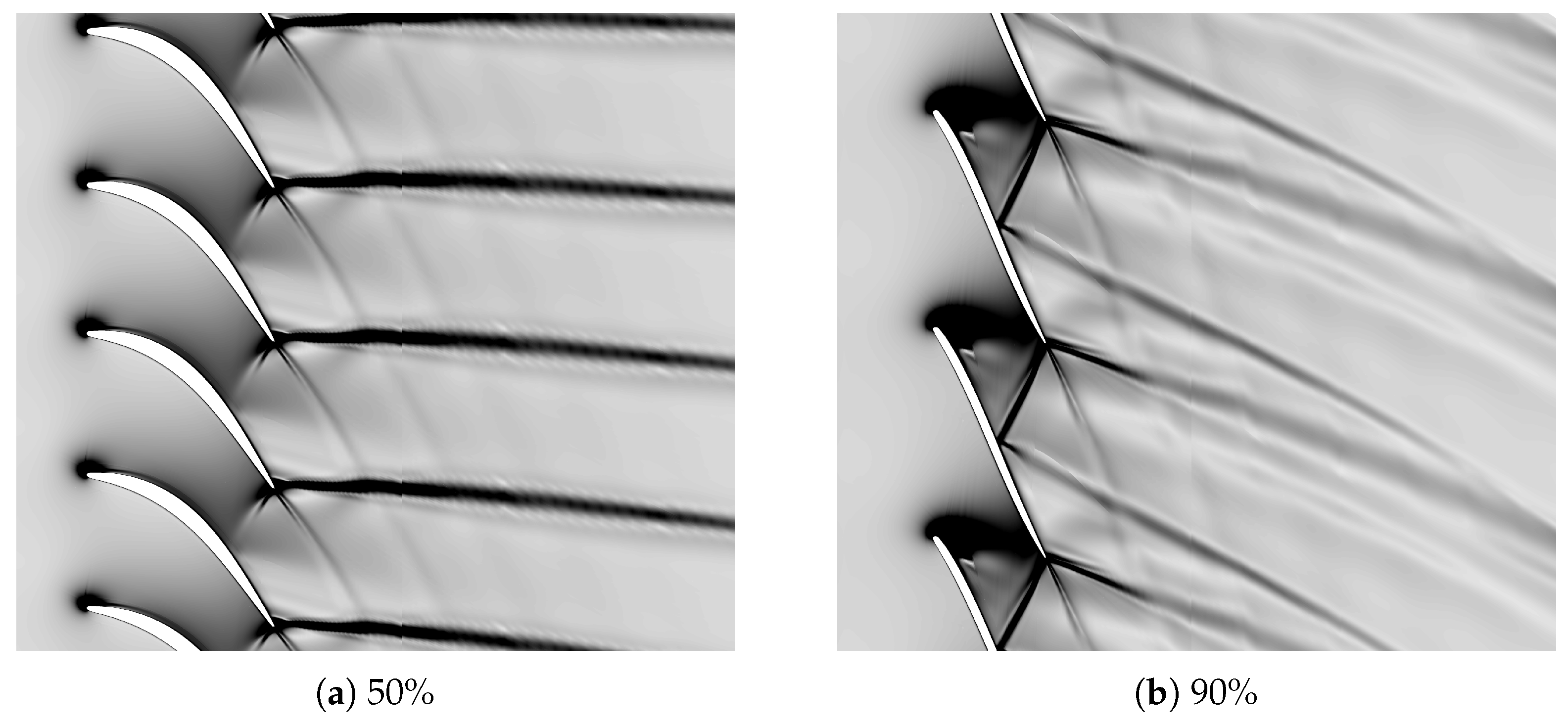
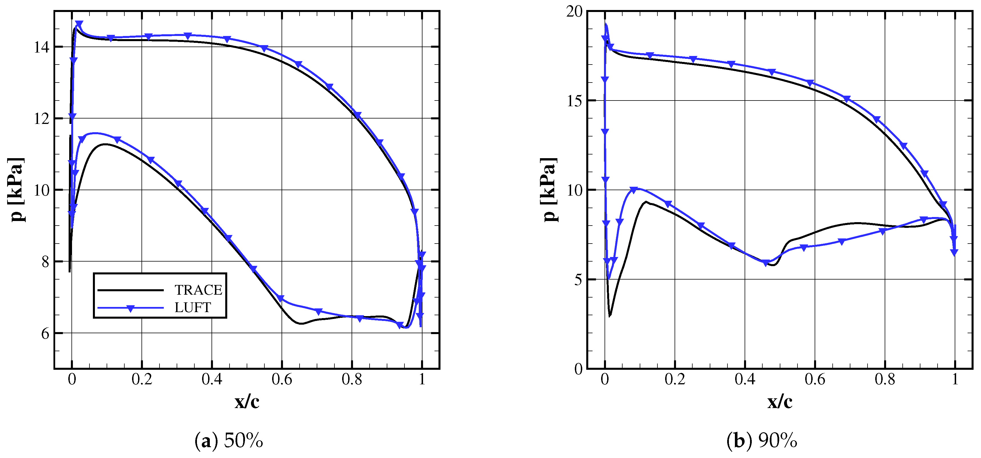
4. Results
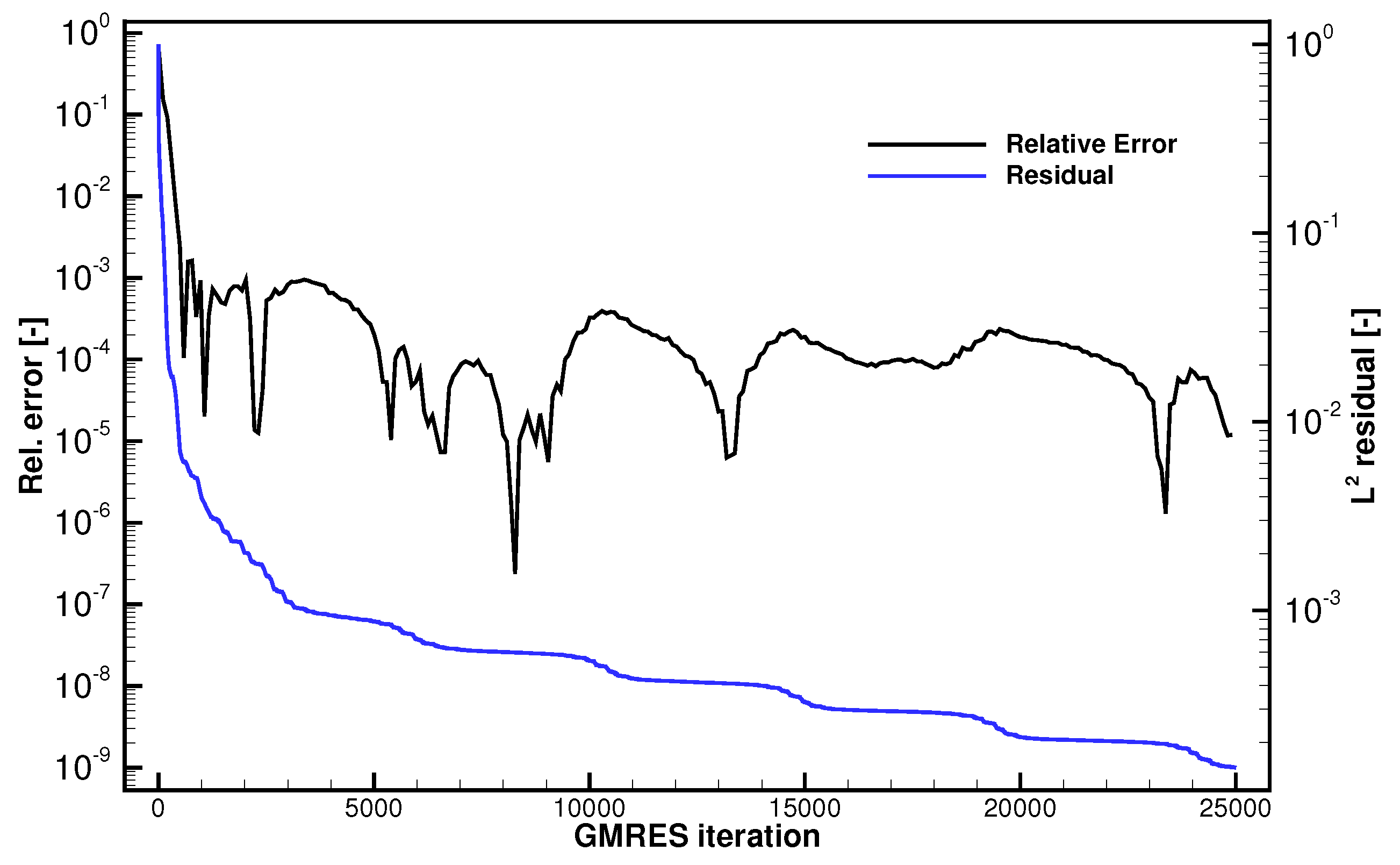
4.1. Linear Solver Set-Up and Results
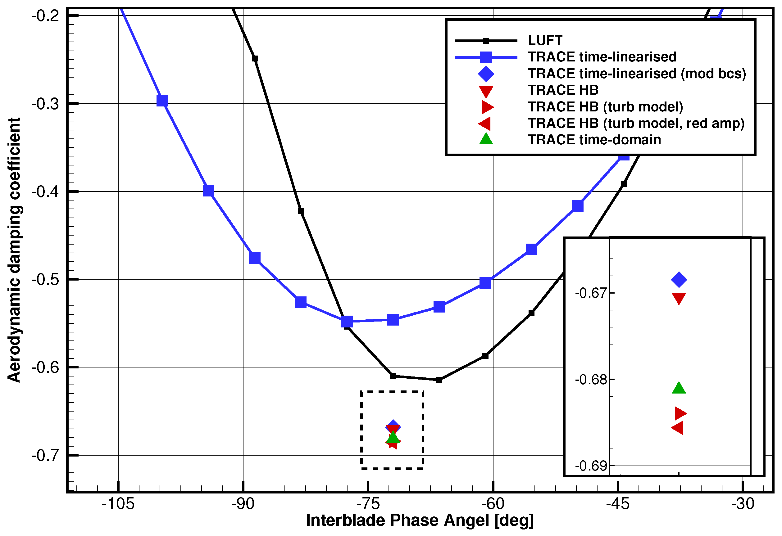
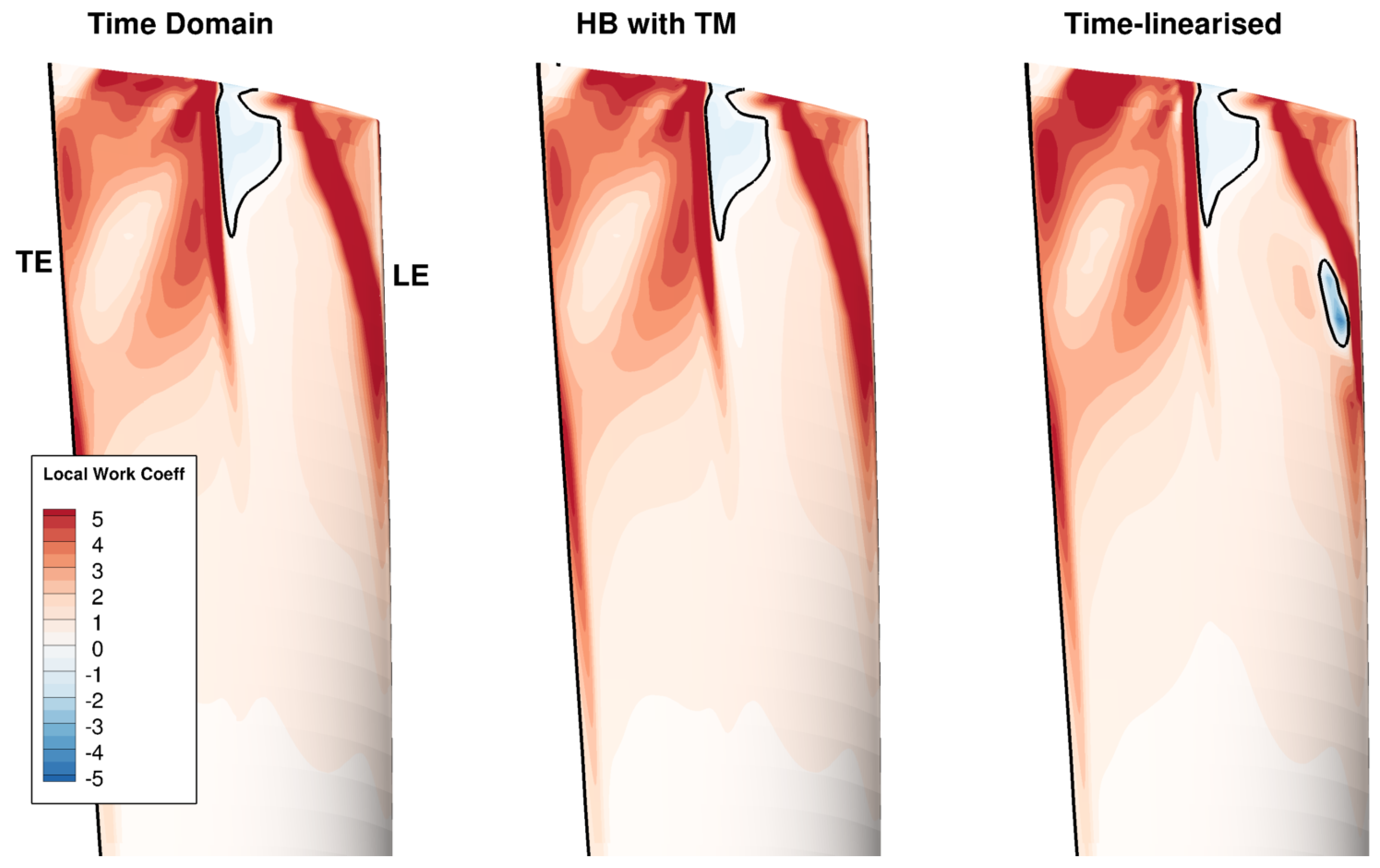
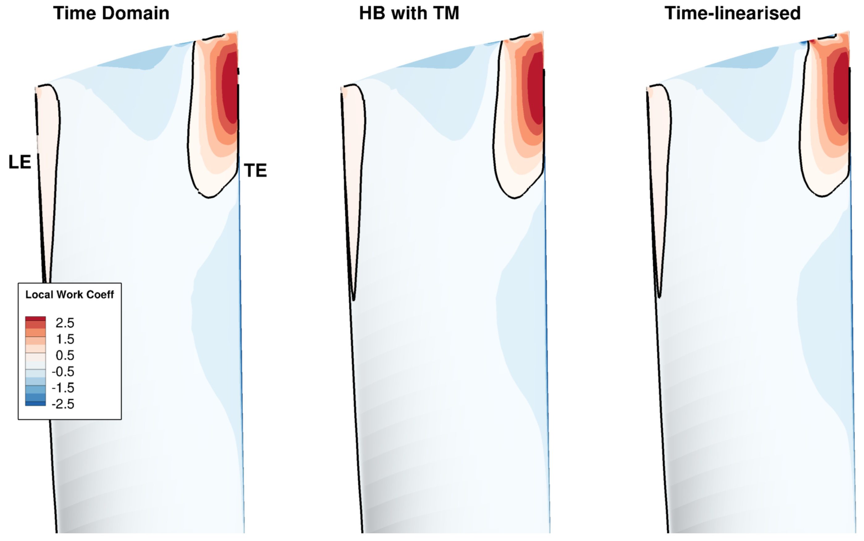
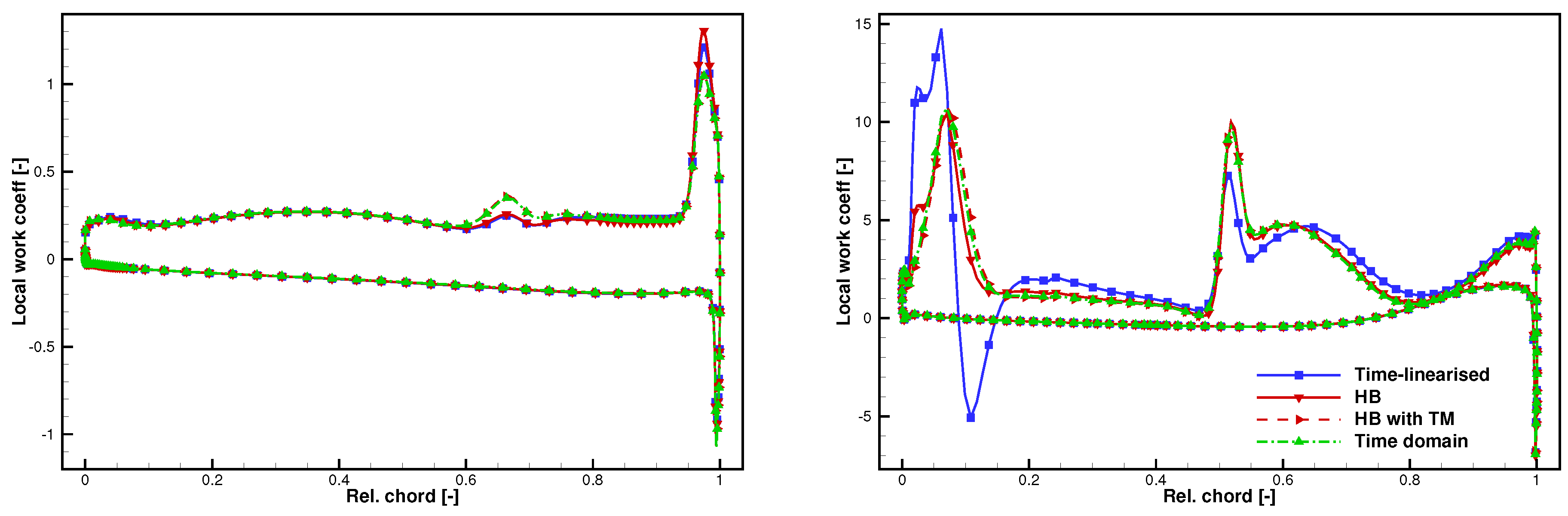
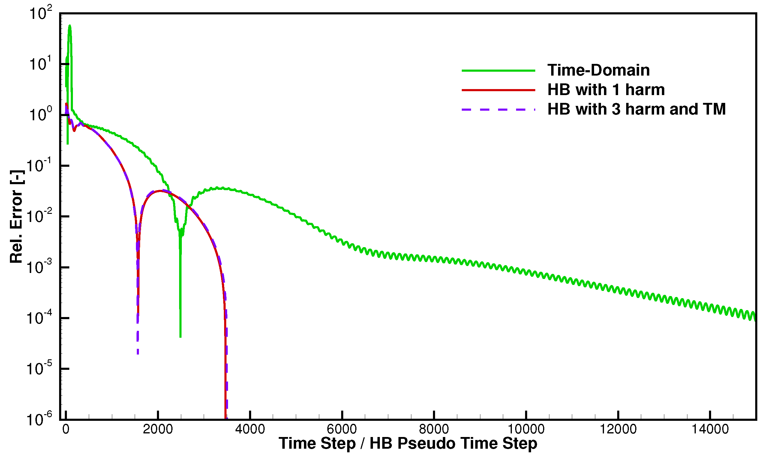
4.2. Harmonic Balance and Time-Domain Results
5. Conclusions
Author Contributions
Funding
Conflicts of Interest
Abbreviations
| HB | Harmonic Balance |
| NRBC | Nonreflecting Boundary Conditions |
Nomenclature
| b | rotor blade height |
| cm | chord at midspan |
| maximal displacement amplitude | |
| vout | velocity magnitude at outlet |
| i | square root of |
| dynamic pressure at rotor inlet | |
| q | vector of conservative flow variables |
| Fourier coefficient of q with respect to the angular frequency | |
| Fourier transform | |
| R | flow residual |
| V | cell volume |
| grid coordinates and velocities | |
| non-dimensionalised amplitude | |
| interblade phase angle | |
| angular frequency |
References
- Rendu, Q.; Philit, M.; Labit, S.; Chassaing, J.C.; Rozenberg, Y.; Aubert, S.; Ferrand, P. Time-Linearized and Harmonic Balance Navier-Stokes Computations of a Transonic Flow over an Oscillating Bump. In Proceedings of the 14th International Symposium on Unsteady Aerodynamics, Aeroacoustics & Aeroelasticity of Turbomachines ISUAAAT14, Stockholm, Sweden, 8–11 September 2015. [Google Scholar]
- Lindquist, D.R. Computation of Unsteady Transonic Flowfields Using Shock Capturing and the Linear Perturbation Euler Equations. Ph.D. Thesis, Department of Aeronautics and Astronautics, Massachusetts Institute of Technology, Cambridge, MA, USA, 1992. [Google Scholar]
- Seeley, C.E.; Wakelam, C.; Zhang, X.; Hofer, D.; Ren, W.M. Investigations of Flutter and Aero Damping of a Turbine Blade: Part 1—Experimental Characterization. In Proceedings of the ASME Turbo Expo 2016: Turbomachinery Technical Conference and Exposition, Seoul, Korea, 13–17 June 2016; number 49842. p. V07BT34A024. [Google Scholar]
- Ren, W.M.; Seeley, C.E.; Zhang, X.; Mitchell, B.E.; Ju, H. Investigations of Flutter and Aero Damping of a Turbine Blade: Part 2—Numerical Simulations. In Proceedings of the ASME Turbo Expo 2016: Turbomachinery Technical Conference and Exposition, Seoul, Korea, 13–17 June 2016; number 49842. p. V07BT34A025. [Google Scholar]
- Schlüß, D.; Frey, C. Time Domain Flutter Simulations of a Steam Turbine Stage Using Spectral 2D Non-reflecting Boundary Conditions. In Proceedings of the 15th International Symposium on Unsteady Aerodynamics, Aeroacoustics and Aeroelasticity of Turbomachines (ISUAAAT), Oxford, UK, 24–27 September 2018. [Google Scholar]
- Burton, Z. Analysis of Low Pressure Steam Turbine Diffuser and Exhaust Hood Systems. Ph.D. Thesis, Durham University, Durham, UK, 2014. [Google Scholar]
- Qi, D.; Petrie-Repar, P.; Gezork, T.; Sun, T. Establishment of an open 3D steam turbine flutter test case. In Proceedings of the 12th European Conference on Turbomachinery Fluid dynamics & Thermodynamics, Stockholm, Sweden, 3–7 April 2017. [Google Scholar]
- Sun, T.; Petrie-Repar, P.; Qi, D. Investigation of Tip Clearance Flow Effects on an Open 3D Steam Turbine Flutter Test Case. In Proceedings of the ASME TurboExpo 2017, Charlotte, NC, USA, 26–30 June 2017; number 50954. p. V008T29A024. [Google Scholar]
- Fuhrer, C.; Vogt, D.M. On the Impact of Simulation Approaches on the Predicted Aerodynamic Damping of a Low Pressure Steam Turbine Rotor. In Proceedings of the ASME TurboExpo 2017, Charlotte, NC, USA, 26–30 June 2017. [Google Scholar]
- Roe, P.L. Approximate Riemann solvers, parameter vectors, and difference schemes. J. Comput. Phys. 1981, 43, 357–372. [Google Scholar] [CrossRef]
- van Leer, B. Towards the ultimate conservative difference scheme. V. A second-order sequel to Godunov’s method. J. Comput. Phys. 1979, 32, 101–136. [Google Scholar] [CrossRef]
- van Albada, G.D.; van Leer, B.; Roberts, W.W., Jr. A comparative study of computational methods in cosmic gas dynamics. Astron. Astrophys. 1982, 108, 76–84. [Google Scholar]
- Harten, A. High Resolution Schemes for Hyperbolic Conservation Laws. J. Comput. Phys. 1983, 49, 357–393. [Google Scholar] [CrossRef]
- Kersken, H.P.; Frey, C.; Voigt, C.; Ashcroft, G. Time-Linearized and Time-Accurate 3D RANS Methods for Aeroelastic Analysis in Turbomachinery. J. Turbomach. 2012, 134, 051024. [Google Scholar] [CrossRef]
- Frey, C.; Ashcroft, G.; Kersken, H.P.; Voigt, C. A Harmonic Balance Technique for Multistage Turbomachinery Applications. In Proceedings of the ASME Turbo Expo 2014: Turbine Technical Conference and Exposition, Düsseldorf, Germany, 16–20 June 2014; number 45615. p. V02BT39A005. [Google Scholar]
- Ashcroft, G.; Frey, C.; Heitkamp, K.; Weckmüller, C. Advanced Numerical Methods for the Prediction of Tonal Noise in Turbomachinery—Part I: Implicit Runge-Kutta Schemes. J. Turbomach. 2013, 136, 021002. [Google Scholar] [CrossRef]
- Ashcroft, G.; Frey, C.; Kersken, H.P. On the Development of a Harmonic Balance Method for Aeroelastic Analysis. In Proceedings of the 6th European Conference on Computational Fluid Dynamics (ECFD VI), Barcelona, Spain, 20–25 July 2014. [Google Scholar]
- Wilcox, D.C. Reassessment of the Scale-Determining Equation for Advanced Turbulence Models. AIAA J. 1988, 26, 1299–1310. [Google Scholar] [CrossRef]
- Ashcroft, G.; Frey, C.; Kersken, H.P.; Kügeler, E.; Wolfrum, N. On The Simulation Of Unsteady Turbulence And Transition Effects In A Multistage Low Pressure Turbine, Part I: Verification And Validation. In Proceedings of the ASME Turbo Expo 2018 Turbomachinery Technical Conference and Exposition, Oslo, Norway, 11–15 June 2018. [Google Scholar]
- Kersken, H.P.; Ashcroft, G.; Frey, C.; Wolfrum, N.; Korte, D. Nonreflecting Boundary Conditions for Aeroelastic analysis in Time and Frequency Domain 3D RANS Solvers. In Proceedings of the ASME Turbo Expo 2014, Düsseldorf, Germany, 16–20 June 2014. [Google Scholar]
- Schlüß, D.; Frey, C.; Ashcroft, G. Consistent Non-reflecting Boundary Conditions For Both Steady and Unsteady Flow Simulations In Turbomachinery Applications. In Proceedings of the ECCOMAS Congress 2016 VII European Congress on Computational Methods in Applied Sciences and Engineering, Crete Island, Greece, 5–10 June 2016. [Google Scholar]
- Petrie-Repar, P.; Makhnov, V.; Shabrov, N.; Smirnov, E.; Galaev, S.; Eliseev, K. Advanced Flutter Analysis of a Long Shrouded Steam Turbine Blade. In Proceedings of the ASME Turbo Expo 2014: Turbine Technical Conference and Exposition. American Society of Mechanical Engineers, Dusseldorf, Germany, 16–20 June 2014; p. V07BT35A022. [Google Scholar]
- Weber, A.; Sauer, M. PyMesh—Template Documentation. In Technical Report DLR-IB-AT-KP-2016-34, German Aerospace Center (DLR); Institute of Propulsion Technology: Linder Hoehe, Cologne, Germany, 2016. [Google Scholar]
- Department of Energy Technology, KTH Royal Institute of Technology, Stockholm, Sweden. 3D Steam Turbine Flutter Test Case. 2018. Available online: https://www.kth.se/en/itm/inst/energiteknik/forskning/kraft-varme/ekv-researchgroups/turbomachinery-group/aeromech-test-cases/3d-steam-turbine-flutter-test-case-1.706654 (accessed on 18 August 2018).
- Frey, C.; Kersken, H.P. On the Regularisation of Non-reflecting Boundary Conditions near Acoustic Resonance. In Proceedings of the ECCOMAS Congress 2016 VII European Congress on Computational Methods in Applied Sciences and Engineering, Crete Island, Greece, 5–10 June 2016. [Google Scholar]
- Petrie-Repar, P.J.; McGhee, A.M.; Jacobs, P.A. Three-Dimensional Viscous Flutter Analysis of Standard Configuration 10. In Proceedings of the ASME Turbo Expo 2007, Montreal, QC, Canada, 14–17 May 2007. [Google Scholar]


| R | ||
| - | ||
© 2019 by the authors. Licensee MDPI, Basel, Switzerland. This article is an open access article distributed under the terms and conditions of the Creative Commons Attribution NonCommercial NoDerivatives (CC BY-NC-ND) license (https://creativecommons.org/licenses/by-nc-nd/4.0/).
Share and Cite
Frey, C.; Ashcroft, G.; Kersken, H.-P.; Schlüß, D. Flutter Analysis of a Transonic Steam Turbine Blade with Frequency and Time-Domain Solvers. Int. J. Turbomach. Propuls. Power 2019, 4, 15. https://doi.org/10.3390/ijtpp4020015
Frey C, Ashcroft G, Kersken H-P, Schlüß D. Flutter Analysis of a Transonic Steam Turbine Blade with Frequency and Time-Domain Solvers. International Journal of Turbomachinery, Propulsion and Power. 2019; 4(2):15. https://doi.org/10.3390/ijtpp4020015
Chicago/Turabian StyleFrey, Christian, Graham Ashcroft, Hans-Peter Kersken, and Daniel Schlüß. 2019. "Flutter Analysis of a Transonic Steam Turbine Blade with Frequency and Time-Domain Solvers" International Journal of Turbomachinery, Propulsion and Power 4, no. 2: 15. https://doi.org/10.3390/ijtpp4020015
APA StyleFrey, C., Ashcroft, G., Kersken, H.-P., & Schlüß, D. (2019). Flutter Analysis of a Transonic Steam Turbine Blade with Frequency and Time-Domain Solvers. International Journal of Turbomachinery, Propulsion and Power, 4(2), 15. https://doi.org/10.3390/ijtpp4020015