Adjoint-Based Multi-Point and Multi-Objective Optimization of a Turbocharger Radial Turbine ^†

Abstract

This paper presents a gradient-based design optimization of a turbocharger radial turbine for automotive applications. The aim is to improve both the total-to-static efficiency and the moment of inertia of the turbine wheel. The search for the optimal designs is accomplished by a high-fidelity adjoint-based optimization framework using a fast sequential quadratic programming algorithm. The proposed method is able to produce improved Pareto-optimal designs, which are trade-offs between the two competing objectives, in only a few iterations. This is realized by redesigning the blade shape and the meridional flow channel for the respective target while satisfying imposed aerodynamic constraints. Furthermore, a comparative study with an evolutionary algorithm suggests that the gradient-based method has found the global Pareto front at a computational cost which is about one order of magnitude lower.

1. Introduction

The use of the adjoint method [1,2] is nowadays well established for design optimization problems in Computational Fluid Dynamics (CFD). The advantage of the adjoint approach is the efficient computation of sensitivity derivatives of a given objective function at a cost which is essentially independent of the number of design variables. This feature makes the adjoint method attractive to tackle large-scale complex design problems by gradient-based optimization methods. For turbomachinery applications, one of the pioneering works was conducted by Giles et al. [3]. Later on, adjoint-based optimization methods have been developed by other research groups to optimize mainly axial turbomachines with various degrees of complexity, ranging from single blade rows [4,5], including hub endwall contouring [6,7] to multi-row and multi-stage architectures [8,9,10].

Recently, we developed an adjoint-based optimization framework which was successfully used to optimize a turbocharger radial turbine wheel at multiple operating points [11]. In that study, the geometry was parameterized with radial-fibred blades to avoid bending stresses in the blades due to centrifugal forces. While this approach can limit mechanical stresses, it does not take into account the moment of inertia of the wheel. However, the turbine wheel plays a key role in the moment of inertia of the turbocharger assembly. This is due to the high density of the materials that are commonly employed, such as Inconel™ 713c, which can withstand the high temperatures of the exhaust gases. Therefore, minimizing the moment of inertia is critical for improving the transient response of the whole turbocharger. Including the moment of inertia in the design process results in a multi-objective design problem where one objective cannot be improved without penalizing the other, which is shown in this paper using a gradient-based optimization method.

The presence of multiple local optima in the design space is a common argument against the use of gradient-based methods [12]. This is because gradient-based algorithms may converge to a point which is significantly worse than the global optimum. However, the existence of multiple local optima for practical applications based on the Euler or Navier–Stokes equations is problem dependent [13]. For example, Zingg et al. [14] performed a comparative evaluation of a genetic algorithm and a gradient-based algorithm for two-dimensional airfoil sections, including single-point, multi-point, and multi-objective optimization problems. Using different examples with different numbers of design variables and constraint convergence criteria, they show that both algorithms reliably converge to the same optimum, but the gradient-based method converges about 5 to 200 times faster. Yu et al. [15] investigated the influence of the initial design on wing aerodynamic shape optimization using the Reynolds-Averaged Navier–Stokes equations. They concluded that the wing geometry of the AIAA Common Research Model [16] is unimodel with a very flat plateau around the optimum using 730 design variables. Similar findings were reported by Koo and Zingg [17] for the same test case by starting from various initial geometries, and they confirm that, unlike previously assumed [18], this design space is not multimodal. On the contrary, Buckley et al. [19] show evidence of two local optima for practical multi-point airfoil design problems. To investigate this point for a realistic turbomachinery design problem, we compare the results of the gradient-based optimization with the outcome of a stochastic evolutionary optimization strategy which has a higher probability to locate the global optimum, but at much larger computational cost.

The remainder of this paper is structured as follows. First, we briefly describe the gradient-based optimization framework. Then, we present the optimization problem and discuss the results. Finally, we draw conclusions from this study.

2. Optimization Framework

A brief summary of the optimization framework is presented below. A more detailed description of the individual components, in particular the geometry parameterization, mesh generation, and the CFD and adjoint solvers can be found in Mueller and Verstraete [11].

2.1. Optimization Algorithm

In this work, the software package SNOPT [20,21] is used. The algorithm employs a Sequential Quadratic Programming (SQP) method in which constraints are directly handled by forming a smooth augmented Lagrangian function [22]. The quadratic subproblem is solved for the optimal point that satisfies the Karush–Kuhn–Tucker optimality condition by a line search procedure. The Hessian of the Lagrangian is approximated by the quasi-Newton Broyden–Fletcher–Goldfarb–Shanno method. SNOPT supports both derivative line search and non-derivative line search techniques. In the present work, the second approach is used which requires only function evaluations to find an appropriate step length based on a quadratic interpolation to solve the optimization problem [21].

2.2. Geometry Parameterization

The geometry parameterization of the radial turbine is accomplished using B-Spline curves and surfaces. The three-dimensional geometry is defined by (1) the meridional flow channel; (2) the camber line surface; (3) a blade thickness distribution which is added normal to the camber line surface to construct the pressure and suction side surfaces; and (4) the number of blades. In particular, the camber line surface is defined by a wrap-angle distribution to enforce a radial blading, which is a common approach in radial turbine design in order to avoid bending stresses in the blades due to centrifugal forces. The position of the B-Spline control points is the design variable which can be modified by the optimizer in a predefined range.

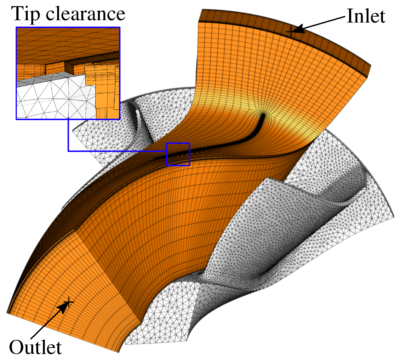
2.3. Mesh Generation

Two different approaches are employed for the discretization of the fluid and solid domains, as shown in Figure 1. For the fluid domain, a three-dimensional multiblock structured grid is used, which is created by stacking annular surface grids. Each surface grid is generated using conformal mapping [23] and two-dimensional elliptic grid generation [24] where source terms are introduced to meet common grid quality standards, e.g., first cell spacing and orthogonality, cell skewness and expansion ratio. The computational cost is reduced by modeling only one blade pitch and using periodic boundary conditions in circumferential direction. In total, 84 layers of cells are used in the span-wise direction, including 20 cells to model the tip clearance. The total number of cells is about 1.1 million. The average wall-spacing is y${}^{+}\approx 1$ and the maximum cell expansion ratio is limited to 1.2 for 20 cells in the O-grid around the blade.

The solid domain is discretized by an unstructured grid using Delaunay triangulation, which is described in more detail by Verstraete et al. [25].

2.4. Analysis Methods

2.4.1. CFD and Adjoint Solver

The governing equations are the compressible Reynolds-Averaged Navier–Stokes (RANS) equations discretized using a cell-centered finite volume formulation on multiblock structured grids. The inviscid fluxes are evaluated by a Roe-type upwind scheme [26] with the entropy correction of Harten and Hyman [27] and a MUSCL reconstruction [28] for second-order spatial accuracy. A van-Albada type limiter [29] is used to suppress oscillations. Viscous fluxes are centrally discretized and the negative Spalart–Allmaras turbulence model [30] is used for the turbulence closure problem assuming a fully turbulent flow from the inlet ($R{e}_{inlet}\approx$ 250,000 based on the turbine wheel diameter). For pseudo-time integration, the JT-KIRK scheme proposed by Xu et al. [31] is used. The developed discrete adjoint solver employs the same time-stepping scheme as the flow solver and features similar performance characteristics in terms of run-time and memory footprint. To simplify the implementation, the constant eddy viscosity (CEV) assumption has been adopted in the adjoint solver. The influence of this approximation has been assessed for the present application by comparing the adjoint-based gradients with gradients computed with the complex-step method [32,33], and a good agreement was observed [11]. A complete description of the CFD and adjoint solvers, including validation, can be found in Ref. [34].

2.4.2. Moment of Inertia Computation

The moment of inertia of the turbine wheel with respect to the axis of rotation is computed with an algorithm proposed by Tonon [35]. It employs explicit formulas using the coordinates of the tetrahedral elements of the solid unstructured mesh. The algorithm provides the exact moment of inertia of the discretized geometry at low computational cost.

2.5. Gradient Evaluation

In this work, the gradient of an aerodynamic cost function J with respect to the design variables $\mathbf{\alpha }$ is evaluated by a two-step approach which decouples the adjoint solver from the geometry and grid generation:

$$\frac{\mathrm{d}J}{\mathrm{d}\mathbf{\alpha }}=\frac{\mathrm{d}J}{\mathrm{d}\mathbf{X}}\frac{\mathrm{d}\mathbf{X}}{\mathrm{d}\mathbf{\alpha }}.$$

(1)

The sensitivity of the cost function with respect to the grid point coordinates ($\mathrm{d}J/\mathrm{d}\mathbf{X}$) is computed by the adjoint solver for each objective and constraint. The complementary sensitivity information of the grid to the design variables ($\mathrm{d}\mathbf{X}/\mathrm{d}\mathbf{\alpha }$) is computed with the complex-step method. Although the computational cost of the complex-step method is proportional to the number of design variables, it is considered feasible due to the limited number of design variables used in this study, as is shown later. Additionally, because the moment of inertia is evaluated by explicit formulas, its gradient with respect to the design variables is obtained at negligible costs using the complex-step method.

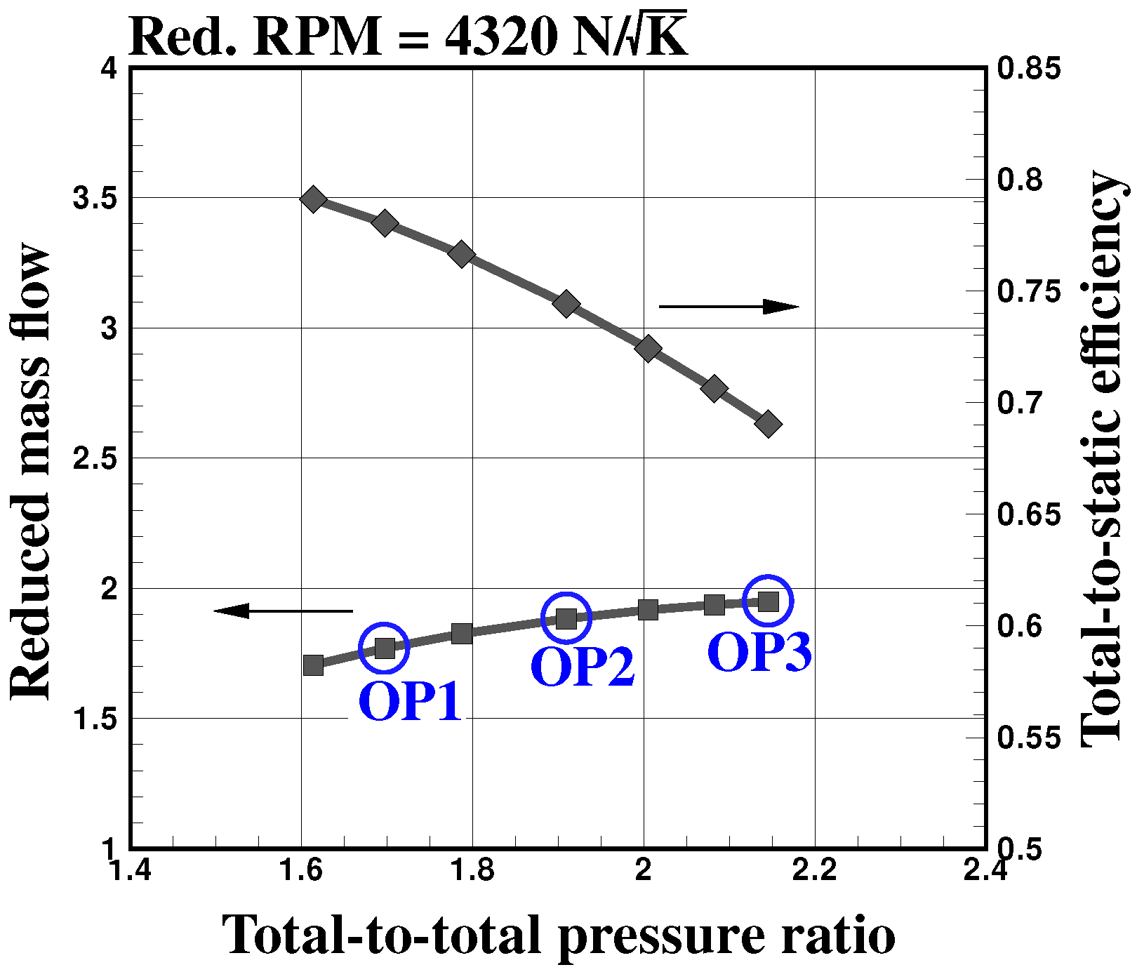
3. Problem Statement

The objective of this study is to maximize the total-to-static efficiency of the turbine wheel at two operating points while minimizing its moment of inertia. Additionally, aerodynamic constraints are imposed such that the optimized wheel delivers the required output power and the swallowing capacity. The operating points are indicated in the performance map of the turbine in Figure 2 and the corresponding boundary conditions are listed in

Table 1. Definition of boundary conditions shown in Figure 2.

Parameter	Symbol	Unit	OP1	OP2	OP3
Inlet flow angle 1	${\alpha }_1$	[${}^{\circ }$]	62
Inlet total pressure	$P_{01}$	[bar]	-	-	3.0
Inlet mass flow	$\dot{m}$	[g/s]	100	130	-
Inlet total temperature	$T_{01}$	[K]	1050
Exit static pressure 2	$P_2$	[bar]	1.013
Rotational speed	$RPM$	[min−1]	140,000

${}^1$ With respect to the radial direction; ${}^2$ Specified at the hub.

. Note that at the operating points OP1 and OP2 the mass flow is directly imposed at the inlet in order to maintain the performance characteristics at these conditions during the optimization process. Additionally, concerning the efficiency, a higher priority is placed on the operating point OP1 because the turbine is expected to operate mostly under this condition. At operating point OP3, the total-to-static pressure ratio is prescribed and the computed mass flow should not be smaller than the baseline design value. The resulting optimization problem may be written as follows:

$$\begin{array}{ccc}\hfill \mathrm{Maximize}:Obj& \equiv & {\omega }_J\underset{Ob{j}_{\mathrm{Efficiency}}}{\underbrace{\left(\frac{2}{3}\frac{{\eta }_{\mathrm{TS},\mathrm{OP}1}}{{\eta }_{\mathrm{TS},\mathrm{OP}1,\mathrm{ref}}}+\frac{1}{3}\frac{{\eta }_{\mathrm{TS},\mathrm{OP}2}}{{\eta }_{\mathrm{TS},\mathrm{OP}2,\mathrm{ref}}}\right)}}+\left(1-{\omega }_J\right)\underset{Ob{j}_{\mathrm{Inertia}}}{\underbrace{\left(1-\frac{I_{\mathrm{xx}}}{I_{\mathrm{xx},\mathrm{ref}}}\right)}},\hfill \\ \hfill \mathrm{Subject}\mathrm{to}:Const{r}_1& \equiv & \left|\frac{{\dot{W}}_{\mathrm{OP}1}}{{\dot{W}}_{\mathrm{OP}1,\mathrm{ref}}}-1\right|\le 0.5\%,\hfill \end{array}$$

(2)

$$\begin{array}{ccc}\hfill Const{r}_2& \equiv & \left|\frac{{\dot{W}}_{\mathrm{OP}2}}{{\dot{W}}_{\mathrm{OP}2,\mathrm{ref}}}-1\right|\le 0.5\%,\hfill \\ \hfill Const{r}_3& \equiv & \frac{{\dot{m}}_{\mathrm{OP}3}}{{\dot{m}}_{\mathrm{OP}3,\mathrm{ref}}}-1\ge 0,\hfill \end{array}$$

(3)

where ${\eta }_{\mathrm{TS}}$, $\dot{W}$, $\dot{m}$ are respectively the total-to-static isentropic efficiency, the power, and the mass flow. The optimization problem is solved with respect to 40 design parameters (Mueller and Verstraete [11]).

The weighting coefficient ${\omega }_J\in [0,1]$ in Equation (2) is a blending factor between the moment of inertia and efficiency term. Setting ${\omega }_J$ = 1 defines an optimization problem which only maximizes the efficiency, whereas the other extreme would result in a formulation that solely focuses on the inertia without taking into account the aerodynamic performance. Its choice is crucial, since it ultimately determines the outcome of the optimization process.

4. Results

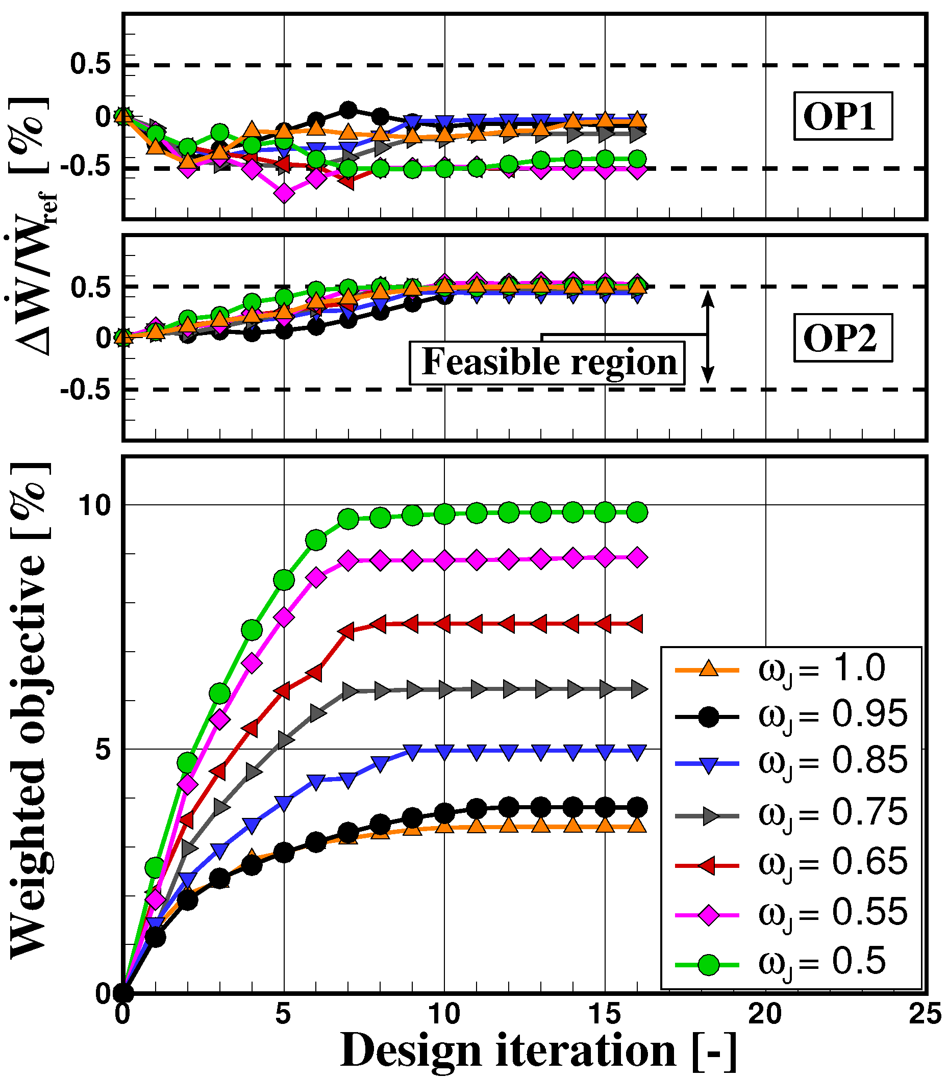
4.1. Optimization History

In order to find different trade-off solutions of this design problem, seven optimization runs have been performed using different weights in the objective function between ${\omega }_J$ = 1.0 and ${\omega }_J$ = 0.5. Figure 3 (bottom) shows the evolution of the weighted objective for each individual run. All final geometries after 16 iterations satisfy the imposed aerodynamic constraints. The computed mass flow at operating point OP3 was always larger than the baseline value, therefore the mass flow constraint was not active throughout the entire optimization process. The power constraints, on the other hand, were active, in particular at the operating point OP2 where the value has reached the upper limit of the imposed bounds in most of the cases, as shown in Figure 3 (top). From Figure 3 (bottom), we can see that giving a higher priority to the moment of inertia (lower ${\omega }_J$) leads to overall larger improvements of the weighted objective function, from 3.5% to almost 10%, compared to the baseline geometry. These results were obtained after almost ten iterations (or even earlier) for each optimization run with minor improvements in the subsequent iterations.

To identify the different trade-offs between low moment of inertia and high efficiency, we further plot the two-dimensional objective space in Figure 4 with the individual components of the weighted objective function. This figure summarizes the results of all optimization runs, including the final designs as well as their search histories in the objective space during the optimization.

As can be seen, depending on the chosen weight, the final design is a trade-off solution between the low moment of inertia and high total-to-static efficiency, establishing a Pareto front towards the lower left hand corner. Once this front is reached, one objective cannot be improved without penalizing the other. The highest aerodynamic performance is obtained when the moment of inertia is excluded during the optimization (${\omega }_J$ = 1.0). Even for this design, however, the moment of inertia could be reduced, i.e., improved by about 10% compared to the baseline design. This is mainly due to the modified hub shape, as is shown later, which has a low impact on the efficiency, but large contribution to the reduced moment of inertia. When reducing the weight, the inertia is further improved at the expense of lower efficiency. For the intermediate case with a weight of ${\omega }_J$ = 0.65, the moment of inertia has improved by approximately 16%, but the total-to-static efficiency is still more than 3% higher compared to the datum geometry. Reducing the weight further diminishes the efficiency gains more rapidly, and for the last optimization run in which an equal weight was given to both objectives, the efficiency improvements have reduced considerably to about 0.9%. In this case, the moment of inertia has improved by about 19%. However, further improvements of the moment of inertia are difficult to realize within the imposed design space, and would eventually come at the price of lower efficiency compared to the baseline design.

The Pareto front shown in Figure 4 has two distinct shapes: one convex part between ${\omega }_J\approx 1.0-0.65$ and one part in which efficiency and the moment of inertia are almost linearly connected (${\omega }_J\approx 0.65-0.5$). The search histories of the two optimization runs using a weight of ${\omega }_J=0.55$ and ${\omega }_J=0.5$ are particularly interesting. Once the optimization algorithm had identified a solution on the Pareto front, the further quest involved marching along the Pareto front in order to find the desired Pareto optimal point that corresponds to the specific weight.

The influence of the weight coefficient on the optimization results is further discussed below. In particular, three values are considered: the minimal and maximal values, ${\omega }_J=0.5$ and ${\omega }_J=1.0$, respectively, as well as an intermediate case with ${\omega }_J=0.75$.

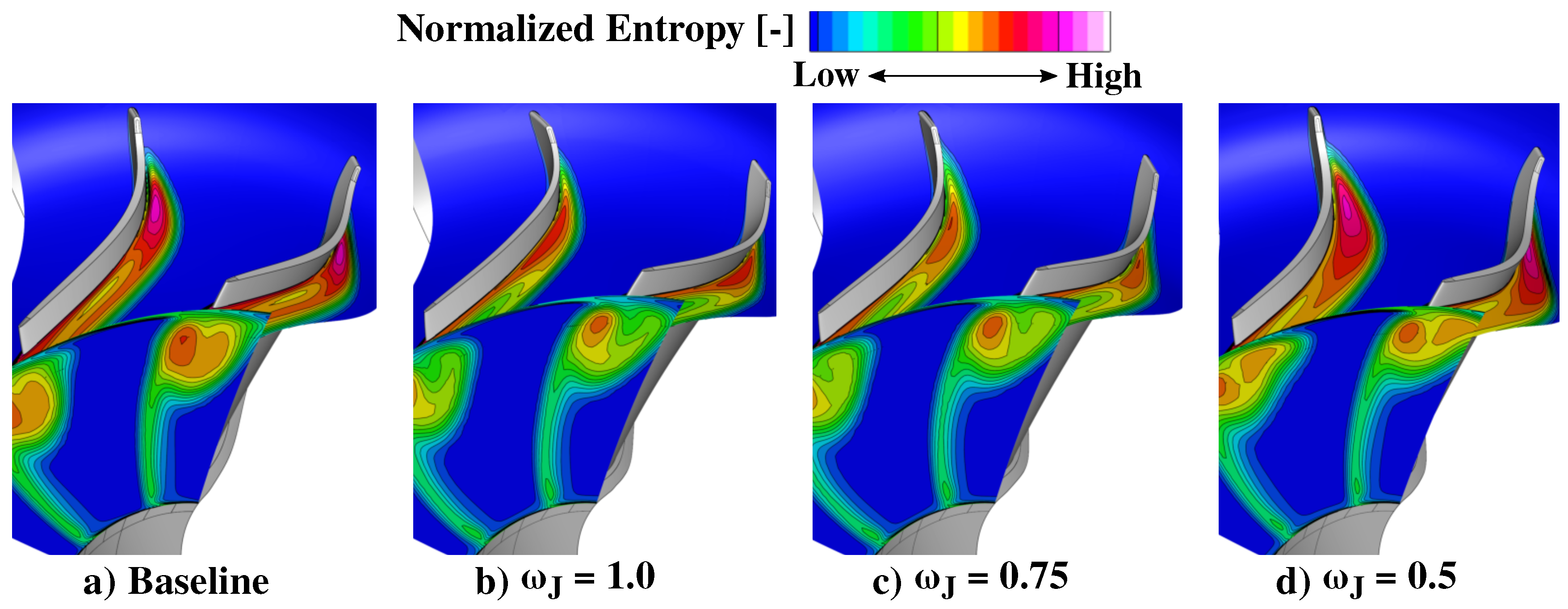
4.2. Influence of the Weight Coefficient

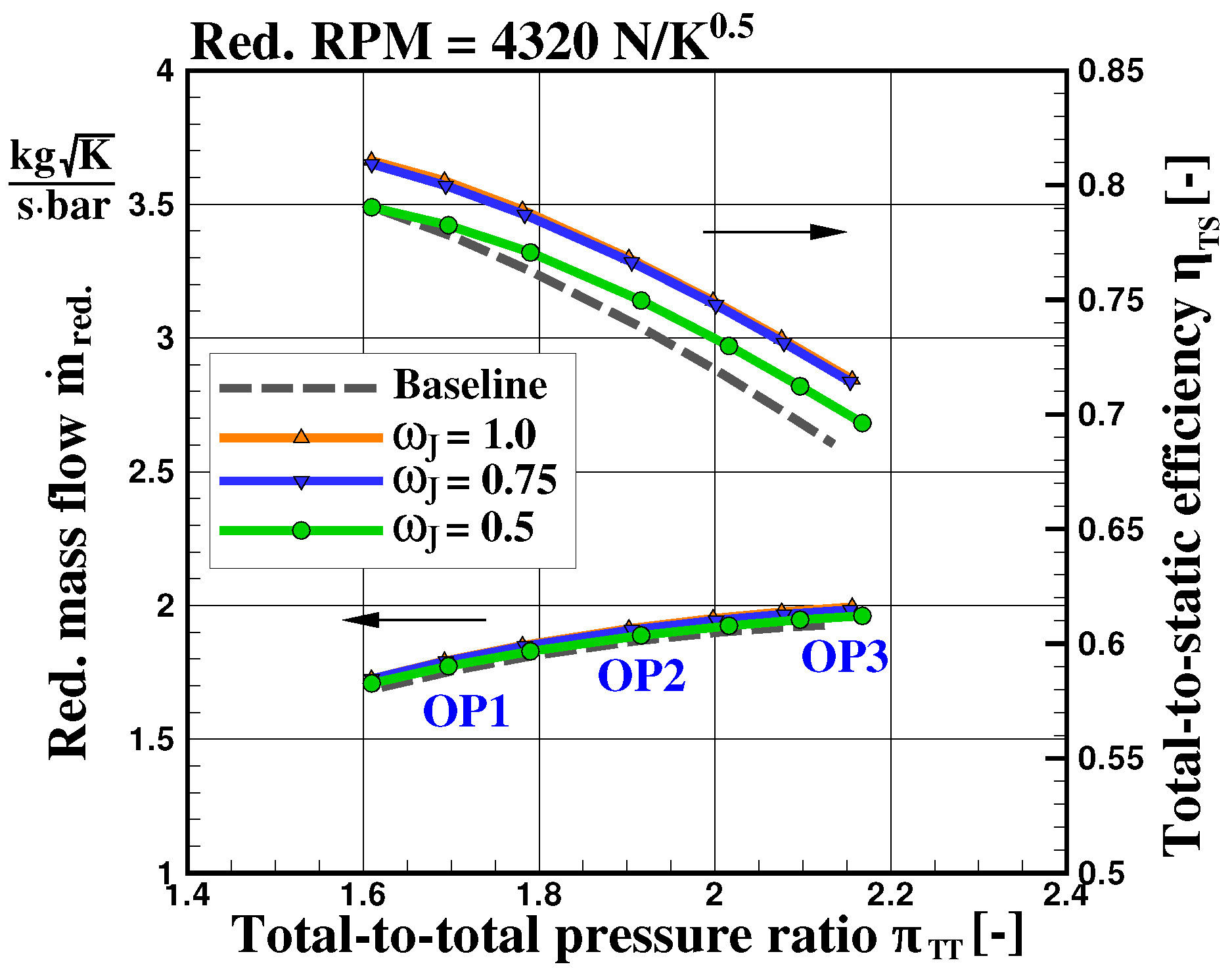
4.2.1. Performance Map

Figure 5 compares the performance map of the baseline and the three optimized geometries with a weight coefficient ${\omega }_J$ of 1.0, 0.75, and 0.5, respectively. In general, in each optimization run the total-to-static efficiency could be increased over the entire investigated operating range compared to the baseline turbine wheel. Due to the scale used in this plot, the performance curves of the optimized designs using a weight coefficient ${\omega }_J$ of 1.0 and 0.75 are almost indistinguishable. In both cases, the total-to-static efficiency is more than three percent points higher compared to the baseline geometry. The efficiency curve of the third optimal geometry (${\omega }_J$ = 0.5), is lower than for the previous two designs. For this particular design, it is noticeable that the total-to-static efficiency has increased at higher mass flow rates relative to the reference geometry while being almost equally efficient at low mass flow rates. Although the objective did not explicitly take into account the efficiency at operating point OP3, it has increased due to lower kinetic energy losses, resulting from an increased exit width which is discussed below.

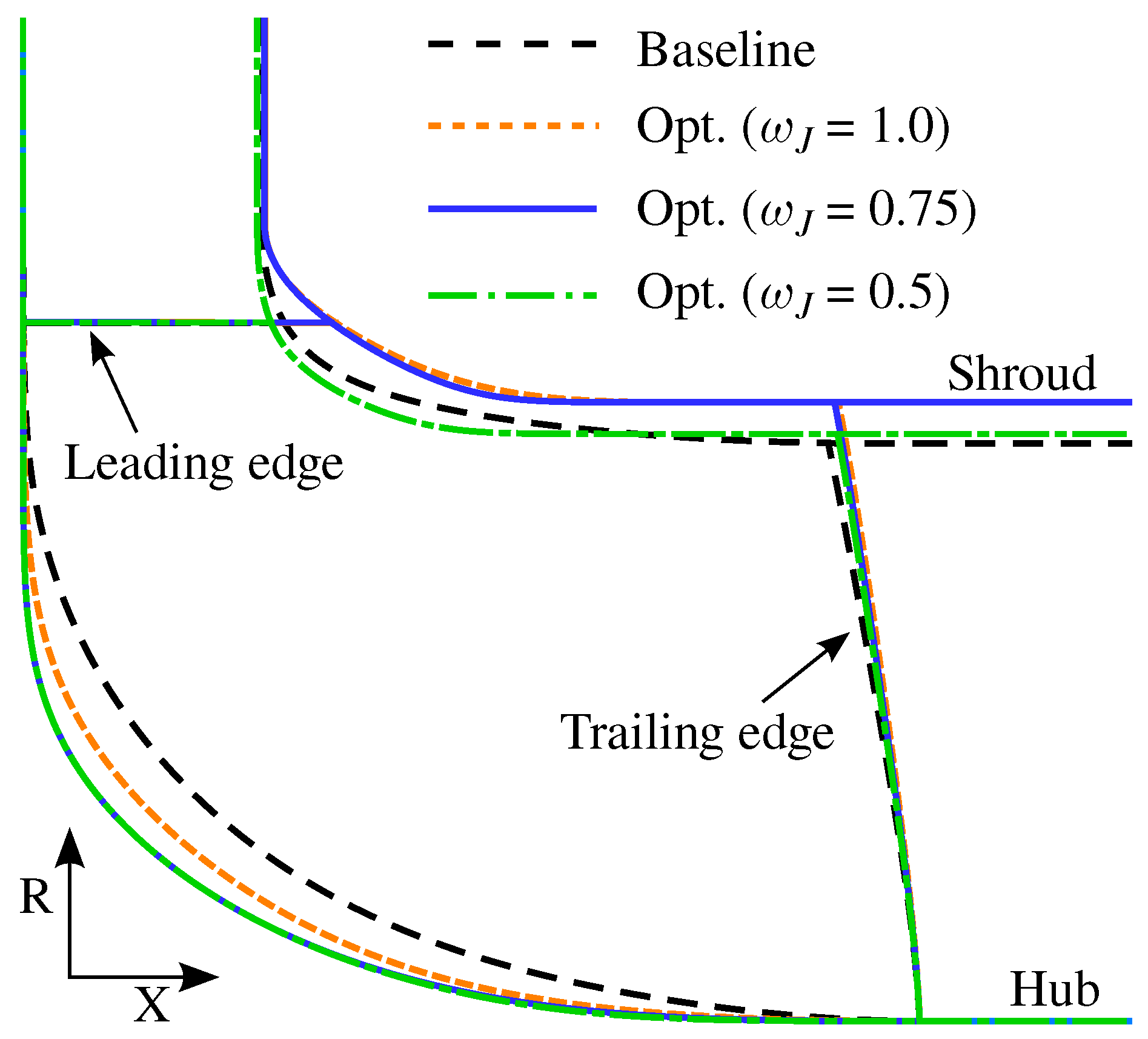
4.2.2. Meridional Shape

Figure 6 compares the meridional shapes of the three optimized geometries with the baseline design. The following conclusions can be drawn: First, the hub shape has been lowered as much as possible when the moment of inertia is included in the weighted objective function (${\omega }_J<1.0$). For the weight coefficient of ${\omega }_J=0.75$, and consequently for ${\omega }_J=0.5$ as well, the hub curve is located at the minimum possible radius inside the imposed design space. Even when a higher weight of ${\omega }_J=0.95$ is used, which is not included in this figure, the same hub shape is obtained. Secondly, the optimal shroud curve depending on the chosen weight coefficient is less predictable due to the conflicting aerodynamic and structural objectives. The final design by using a weight of ${\omega }_J=0.75$ has the same, i.e., maximum possible exit width as the best efficiency design (${\omega }_J=1.0$). The only noticeable difference between these two designs is in the front part of the blade where the design resulting from ${\omega }_J=0.75$ has slightly shorter blades in favor of a lower moment of inertia. The final design using a weight coefficient of ${\omega }_J=0.5$ has a smaller exit width compared to the other two optimized geometries. However, it is still higher than for the baseline geometry in order to reduce the exit kinetic energy losses, and thus to increase the total-to-static efficiency. On the other hand, this design has shorter blades in the front part, which leads to a lower moment of inertia due to less material at higher radius.

4.2.3. Blade Shape

Finally, the influence of the weighting coefficient on the blade shape is discussed. For this purpose, the three-dimensional geometries of the three optimized designs are shown in Figure 7. A clear trend can be observed that, starting from the left to the right of this figure, the blade bending has been reduced by the optimizer as the weight coefficient is being reduced from ${\omega }_J=1.0$ to ${\omega }_J=0.5$. As a consequence, the blade chord length is reduced, which results in overall shorter blades with a lower moment of inertia. This is especially true in the front part, where the optimized blade becomes more straight when the weight coefficient is reduced. However, in the rear part of the blade, the blade bending, and thus the exit blade metal angle has been reduced less in order to provide enough flow turning to generate the required output power.

The loss generation inside the baseline and the optimized turbine wheels is shown in Figure 8 by means of the normalized entropy generation at 80% span height and downstream of the blade. Compared to the baseline design, the lower losses in the optimized wheel using a weight coefficient of ${\omega }_J=1.0$ are mainly due to a redistributed blade loading and weaker tip leakage vortex. This results in an attenuated wake downstream of the blade visible in Figure 8b near the shroud endwall. A similar flow structure can be observed for the second optimized design (${\omega }_J=0.75$), which is almost equally efficient as the first optimized design from an aerodynamic perspective, but has about 5% lower moment of inertia. However, for the third optimized design (${\omega }_J=0.5$) shown in Figure 8d, there are additional losses accumulated on the suction-side surface due to a small separation bubble at the blade leading edge. The separation bubble is caused by too large positive incidence, which is a result of having radial blade leading edges in combination with a meridional flow channel discussed earlier.

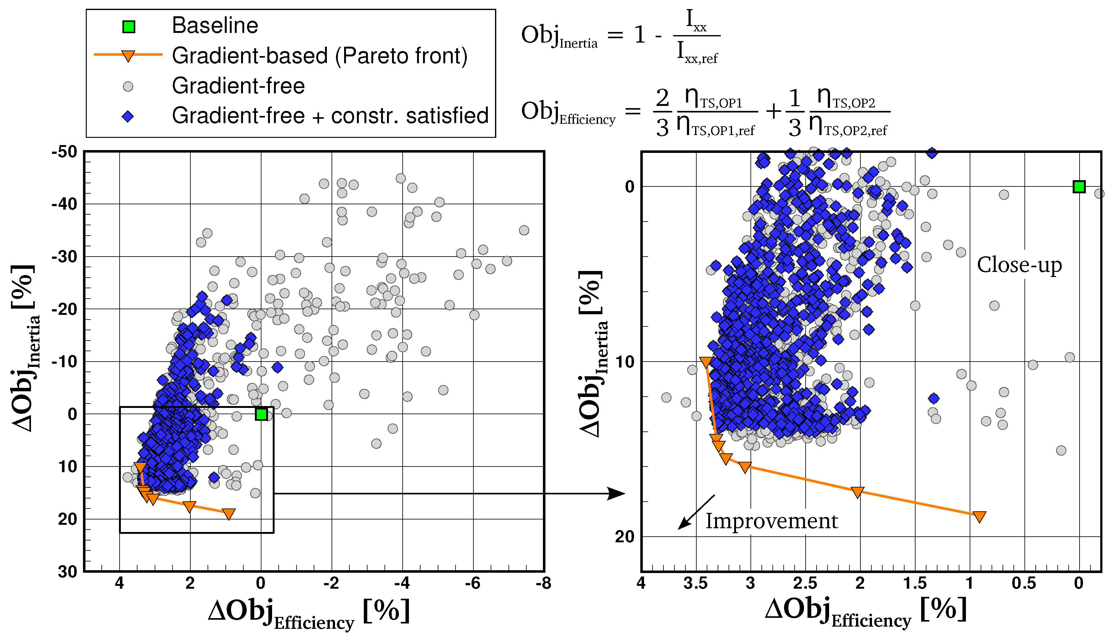
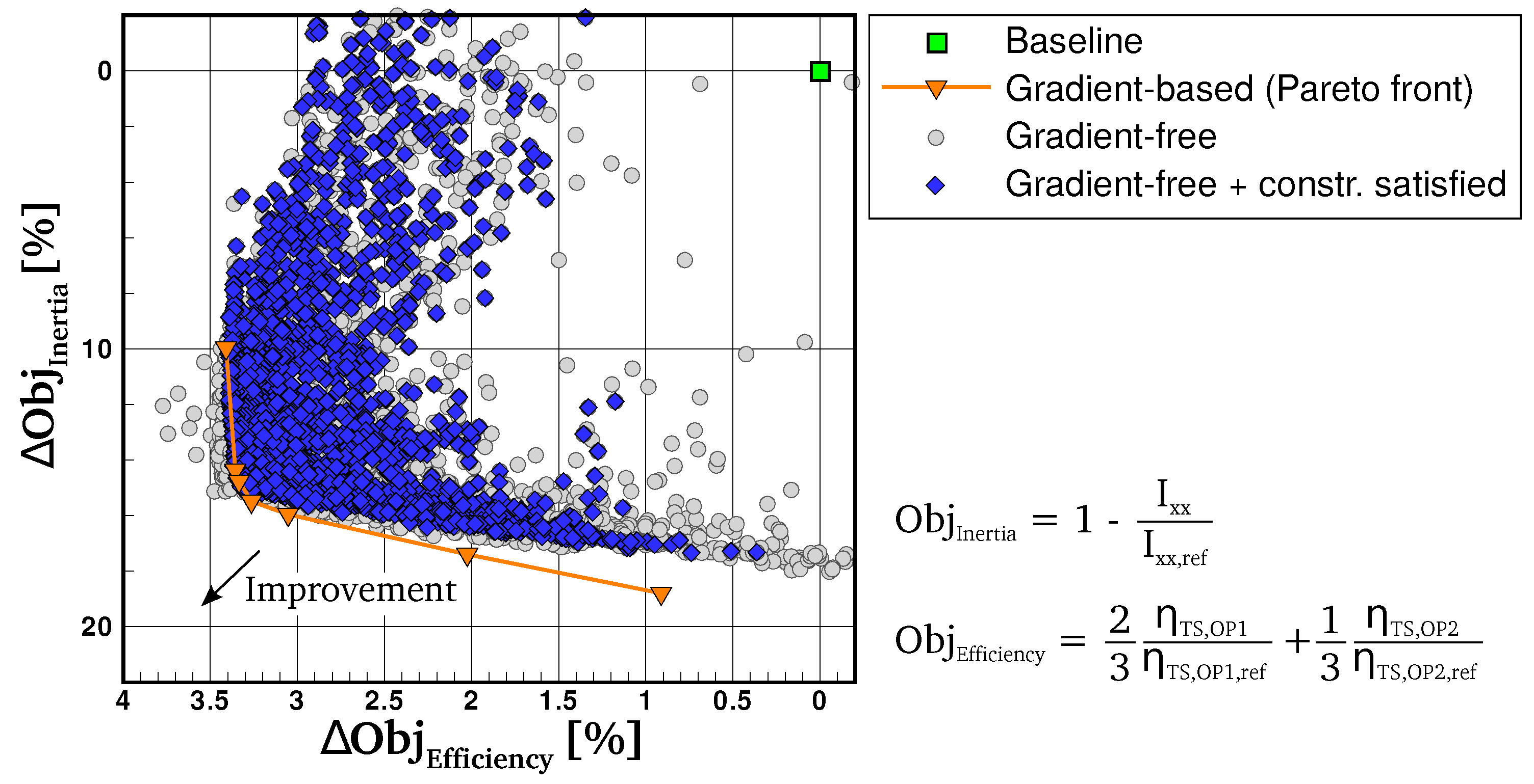
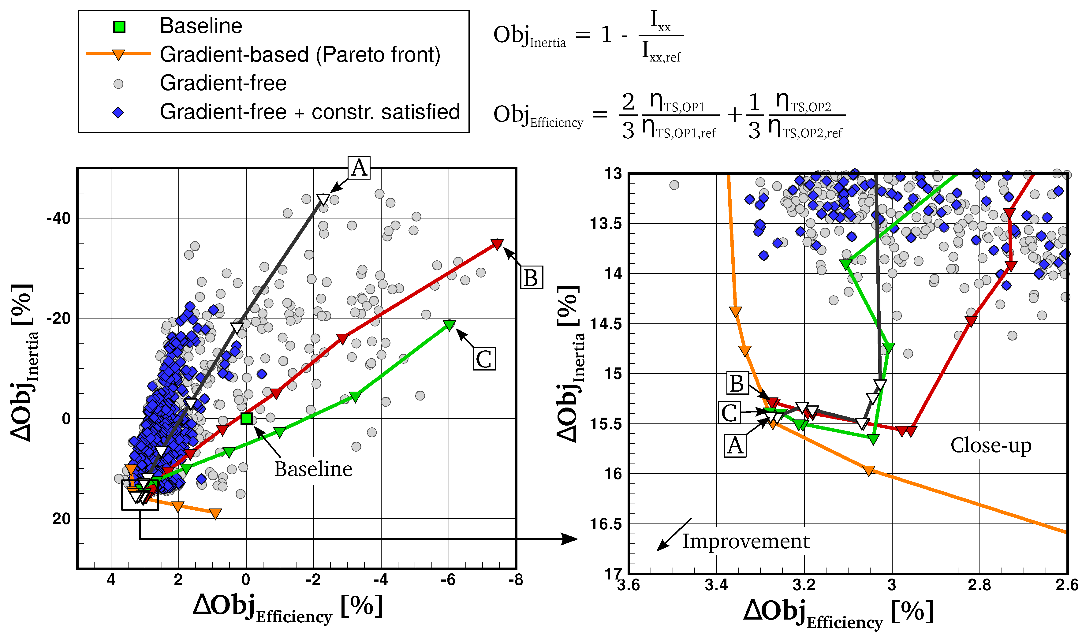
4.3. Comparison with the Gradient-Free Optimization Algorithm

As already mentioned in the introduction, gradient-based optimization algorithms can get trapped in a local optimum rather than finding the best possible design in a given design space. To verify this for the current design problem, the results from the previous section are compared with the outcome of a global optimization strategy. For this purpose, the Differential Evolution (DE) algorithm developed by Storn and Price [36] is used, which is implemented in the VKI optimization framework CADO [37]. Like all evolutionary methods, DE algorithms explore the search space by evolving the population by mechanisms such as mutation, crossover, and selection. Thus, at each generation, the algorithm requires the evaluation of the entire population of designs. The DE algorithm simultaneously optimizes both objectives by employing the non-dominating sorting genetic algorithm [38]. In the present study, a constant population size of 30 individuals was chosen, resulting in an overall computational cost of 90 CFD calculations per generation (30 designs × 3 operating points). Due to the tight convergence criteria of the power constraints at the first and second operating point (cf. Equation (3)), no surrogate models were used during the optimization.

4.3.1. Results after 80 Generations

Figure 9 (left) shows the two-dimensional objective space after 80 generations of the DE algorithm together with the baseline design and the Pareto front established by the gradient-based optimization strategy. The circle symbols represent all designs generated by the DE algorithm, labeled Gradient-free. Moreover, designs which satisfy the aerodynamic constraints are indicated by diamond symbols (Gradient-free + constr. satisfied). In total, the DE algorithm evaluated 2400 geometries of which about 1000 individuals are violating at least one of the constraints. In particular, in the early stage of the optimization process, many invalid designs with poor objective function values were tested, which led to the large scatter of samples in the objective space shown in Figure 9 (left). However, as the optimization progressed, more and more improved designs were generated which satisfy the aerodynamic constraints and have higher total-to-static efficiency and a lower moment of inertia than the baseline geometry. Figure 9 (right) is a close-up of the objective space that provides a better view on the Pareto front. The main conclusions are as follows: The DE algorithm was able to capture the left branch of the Pareto front computed by the gradient-based algorithm. In this region, the efficiency objective is about 3.3% higher compared to the baseline design. Given the close agreement between the gradient-based and the gradient-free algorithms, and the fact that the DE algorithm hardly improved the efficiency any further in the last ten generations, this already indicates that the left part of the Pareto front found by the gradient-based algorithm corresponds to the global Pareto front of this optimization problem. On the other hand, a lack of convergence of the DE algorithm is particularly noticeable towards the right branch of the Pareto front, where more emphasis is placed on lowering the moment of inertia. As shown in Figure 9 (right), the moment of inertia improvements stagnate at about 14% relative to the baseline geometry after 80 generations. These improvements are mainly realized by lowering the hub shape, which has a large impact on the moment of inertia.

This is more clearly shown in Figure 10, which compares the meridional shapes of three designs (A, B, C) located on this front with the baseline geometry. The hub shape of all three designs is located almost at the smallest possible radial position in the design space. At the same time, the DE algorithm increased the exit width compared to the baseline geometry in order to improve the total-to-static efficiency. The efficiency differences between the designs A, B, and C are due to small differences of the shroud curve at the leading edge, but to a larger extent due to different blade shapes. A further reduction of the moment of inertia beyond the current values after 80 generations requires a combination of lowering the exit width to shorten the blade length as well as reducing the blade chord length, as was shown in the previous section. For the DE algorithm, however, this seems to be difficult, particularly due to the tight convergence criteria of the power constraints at the two operating points (OP1 and OP2), and thus it requires more iterations to further explore the objective space.

4.3.2. Results after 200 Generations

Figure 11 shows a close-up on the Pareto-front in the objective space after 200 generations of the gradient-free algorithm. Compared to the results after 80 generations, the DE algorithm found significantly more geometries with a lower moment of inertia which also satisfy the aerodynamic constraints indicated by the blue diamond-shaped symbols. As shown in this figure, the right branch of the Pareto-front established by the gradient-based method is gradually approached. Additionally, the left branch of the Pareto-front towards higher efficiency is equally captured by both optimization strategies. Overall, these results support the conclusion that the Pareto-front computed by the gradient-based method corresponds to the global one of this optimization problem.

The computational costs of both optimization strategies are compared in

Table 2. Computational cost comparison of the gradient-free (Differential Evolution) algorithm and the gradient-based (Sequential Quadratic Programming) algorithm.

Optimizer		Cost (CFD + Adjoint Evaluations)
Gradient-free		18,000
Gradient-based	${\omega }_J=1.0$	143
	${\omega }_J=0.95$	146
	${\omega }_J=0.85$	140
	${\omega }_J=0.75$	137
	${\omega }_J=0.65$	143
	${\omega }_J=0.55$	155
	${\omega }_J=0.5$	158
		1022 (in total)

. They are measured in terms of the number of CFD and gradient evaluations. The cost of computing the moment of inertia is negligible. The gradient-free optimizer performed in total 18,000 CFD evaluations (200 generations × 30 individuals/generation × 3 operating points/individual). The cost of the gradient-based optimizer includes both CFD evaluations and gradient calculations. As mentioned before, the cost of one adjoint solution is similar to one CFD run both in terms of run-time and memory footprint.

Table 2 lists each optimization run of the gradient-based algorithm separately. In the first case with ${\omega }_J=1.0$, the computational cost is equivalent to 143 CFD evaluations, which corresponds to 16 design iterations with each three CFD and five adjoint calculations. Additionally, five line-search iterations were performed with each three CFD evaluations. In total, the computational cost of all gradient-based optimization runs is equivalent to 1022 CFD evaluations, which is about one order of magnitude lower than for the gradient-free method. Similar findings were reported by Zingg et al. [14] who concluded that the cost of gradient-free algorithms dramatically increases with tighter convergence requirements. In this work, the tight convergence criteria of the power constraints at the two operating points (OP1 and OP2) are one of the main reasons for the large number of required function evaluations by the gradient-free optimizer.

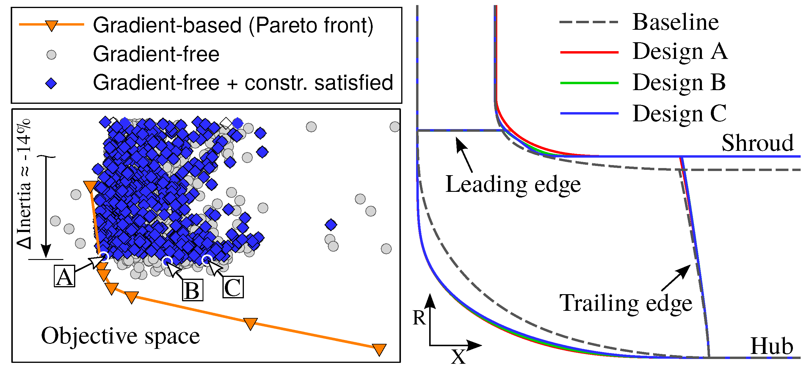
4.3.3. Influence of Initial Design

The results presented in the previous section show that the gradient-based optimization algorithm is able to establish the Pareto front at significantly lower computational cost compared to the gradient-free method. Additionally, the comparison between both optimization strategies suggests that the Pareto optimal designs computed by the gradient-based method correspond to the global optima of this design problem. However, since gradient-based methods converge to the optimum which is closest to the starting point, the question remains whether the Pareto front could only be found due to the initial geometry. To investigate this point, three different geometries generated by the gradient-free algorithm were randomly selected as starting geometries. These geometries are labeled A, B, and C in Figure 12 (left) and are located on the opposite end of the objective space relative to the Pareto front, and therefore exhibit poor aerodynamic and structural performances. Relative to the baseline geometry, these designs have an about 20–40% higher moment of inertia and about 2–8% lower total-to-static efficiency. None of the initial geometries satisfy the aerodynamic constraints. Three independent gradient-based optimization runs have been performed with a weighting coefficient of ${\omega }_J=0.75$ in the weighted objective function.

The search histories are shown in Figure 12. In general, the search histories of each run have similar characteristics: First, starting from the initial geometries (Figure 12, left), the optimizer marches straight through the objective space towards the region of interest. Then, close to the Pareto front, shown in Figure 12 (right), the inertia improvements level off at about $\Delta {\mathrm{Obj}}_{\mathrm{Inertia}}$ = 15.5% relative to the baseline geometry and the optimizer mainly focuses on improving the total-to-static efficiency in the subsequent iterations.

Table 3. Comparison of the final aerodynamic and structural objective values relative to the baseline geometry of the three final designs A, B, and C, shown in Figure 12.

Design	$\mathbf{\Delta }{\mathbf{Obj}}_{\mathbf{Efficiency}}$ [%]	$\mathbf{\Delta }{\mathbf{Obj}}_{\mathbf{Inertia}}$ [%]
A	3.277	15.421
B	3.275	15.298
C	3.279	15.374

summarizes the aerodynamic and structural objective values of the three final designs A, B, and C shown in Figure 12 (right) relative to the baseline geometry. From an aerodynamic point of view, these designs are essentially the same, because the efficiency objective values only differ in the order of $\mathcal{O}\left({10}^{-3}\right)$ percent. Regarding the moment of inertia, the difference between the three designs is about 0.1%. Here, the discrepancies are likely due to the fact that the solid unstructured grid is re-meshed for every new iteration, which changes the number of grid nodes and their connectivity, and therefore introduces small numerical noise in the moment of inertia computation. However, from an engineering perspective, these differences are negligible. Moreover, all final designs A, B, and C satisfy the aerodynamic constraints, suggesting that the design space in this work is convex with one optimum for which gradient-based algorithms are particularly suited due to their computational efficiency.

5. Conclusions

A multi-point and multi-objective gradient-based optimization procedure is proposed and successfully applied to a turbocharger radial turbine for automotive applications. The aim of this design study is to improve the total-to-static efficiency and the moment of inertia of the turbine wheel while maintaining the output power and the swallowing capacity of the machine. The optimization is accomplished by a fast Sequential Quadratic Programming (SQP) algorithm using adjoint sensitivity analysis, which allows an efficient computation of the gradients.

The optimization results show a significant improvement of both objectives in only a few iterations. In particular, the proposed method is able to find Pareto-optimal designs which are trade-offs between the two competing objectives. This is achieved by modifying the blade shape, as well as the hub and shroud endwall contours while satisfying the strict aerodynamic constraints. Furthermore, a comparison with the outcome of a gradient-free evolutionary optimization strategy, in which no surrogate models were used, suggests that the gradient-based method has found the global optimum at a computational cost which is about one order of magnitude lower. Thus, the gradient-based optimization framework proves to be a very efficient design tool.

References

1. Pironneau, O. On Optimum Design in Fluid Mechanics. J. Fluid Mech. 1974, 64, 97–110. [Google Scholar] [CrossRef]
2. Jameson, A. Aerodynamic Design via Control Theory. J. Sci. Comput. 1988, 3, 233–260. [Google Scholar] [CrossRef]
3. Giles, M.B.; Duta, M.C.; Müller, J.-D.; Pierce, N.A. Algorithm Developments for Discrete Adjoint Methods. AIAA J. 2003, 41, 198–205. [Google Scholar] [CrossRef] [Green Version]
4. Papadimitriou, D.I.; Giannakoglou, K.C. Total Pressure Loss Minimization in Turbomachinery Cascades Using a New Continuous Adjoint Formulation. J. Power Energy 2007, 221, 865–872. [Google Scholar] [CrossRef]
5. Marta, A.C.; Shankaran, S.; Holmes, D.G.; Stein, A. Development of Adjoint Solvers for Engineering Gradient-Based Turbomachinery Design Applications. In Proceedings of the ASME Turbo Expo, Orlando, FL, USA, 8–12 June 2009. [Google Scholar]
6. Luo, J.; Liu, F.; McBean, I. Turbine Blade Row Optimization Through Endwall Contouring by an Adjoint Method. J. Propuls. Power 2015, 31, 505–518. [Google Scholar] [CrossRef] [Green Version]
7. Corral, R.; Gisbert, F. Profiled End Wall Design Using an Adjoint Navier-Stokes Solver. J. Turbomach. 2008, 130, 021011. [Google Scholar] [CrossRef]
8. Wang, D.X.; He, L. Adjoint Aerodynamic Design Optimization for Blades in Multi-Stage Turbomachines: Part 1—Methodology and Verification. J. Turbomach. 2010, 132, 021011. [Google Scholar] [CrossRef]
9. Shahpar, S.; Caloni, S. Adjoint Optimisation of a High Pressure Turbine Stage for Lean-Burn Combustion System. In Proceedings of the 10th European Conference on Turbomachinery, Fluid Dynamics and Thermodynamics, Lappeenranta, Finland, 15–19 April 2013. [Google Scholar]
10. Walther, B.; Nadarajah, S. Optimum Shape Design for Multirow Turbomachinery Configurations Using a Discrete Adjoint Approach and an Efficient Radial Basis Function Deformation Scheme for Complex Multiblock Grids. J. Turbomach. 2015, 137, 081006. [Google Scholar] [CrossRef]
11. Mueller, L.; Verstraete, T. CAD Integrated Multipoint Adjoint-Based Optimization of a Turbocharger Radial Turbine. Int. J. Turbomach. Propuls. Power 2017, 2, 14. [Google Scholar] [CrossRef]
12. Namgoong, H.; Crossley, W.; Lyrintzis, A.S. Global Optimization Issues for Transonic Airfoil Design. In Proceedings of the 9th AIAA/ISSMO Symposium on Multidisciplinary Analysis and Optimization, Atlanta, GA, USA, 4–6 September 2002. [Google Scholar]
13. Chernukhin, O.; Zingg, D.W. Multimodality and Global Optimization in Aerodynamic Design. AIAA J. 2013, 51, 1342–1354. [Google Scholar] [CrossRef] [Green Version]
14. Zingg, D.W.; Nemec, M.; Pulliam, T.H. A Comparative Evaluation of Genetic and Gradient-Based Algorithms Applied to Aerodynamic Optimization. Eur. J. Comput. Mech. 2008, 17, 103–126. [Google Scholar] [CrossRef]
15. Yu, Y.; Lyu, Z.; Xu, Z.; Martins, J.R.R.A. On the Influence of Optimization Algorithm and Initial Design on Wing Aerodynamic Shape Optimization. Aerosp. Sci. Technol. 2018, 15, 183–199. [Google Scholar] [CrossRef]
16. Vassberg, J.; Dehaan, M.; Rivers, M.; Wahls, R. Development of a Common Research Model for Applied CFD Validation Studies. In Proceedings of the 26th AIAA Applied Aerodynamics Conference, Honolulu, HI, USA, 18–21 August 2008. [Google Scholar]
17. Koo, D.; Zingg, D.W. Investigation into Aerodynamic Shape Optimization of Planar and Nonplanar Wings. AIAA J. 2018, 56, 250–263. [Google Scholar] [CrossRef]
18. Osusky, L.; Buckley, H.P.; Reist, T.A.; Zingg, D.W. Drag Minimization based on the Navier-Stokes Equations Using a Newton-Krylov Approach. AIAA J. 2015, 53, 1555–1577. [Google Scholar] [CrossRef]
19. Buckley, H.P.; Zhou, B.Y.; Zingg, D.W. Airfoil Optimization Using Practical Aerodynamic Design Requirements. J. Aircr. 2010, 47, 1707–1719. [Google Scholar] [CrossRef] [Green Version]
20. Gill, P.E.; Murray, W.; Saunders, M.A. An SQP Algorithm for Large-Scale Constrained Optimization. SIAM J. Optim. 2002, 12, 979–1006. [Google Scholar] [CrossRef]
21. Gill, P.E.; Murray, W.; Saunders, M.A. User’s Guide for SNOPT Version 7: Software for Large-Scale Nonlinear Programming; University of California: San Diego, CA, USA, 2008. [Google Scholar]
22. Gill, P.E.; Murray, W.; Saunders, M.A. Some Theoretical Properties of an Augmented Lagrangian Merit Function; Technical Report SOL 86-6R; Stanford University: Stanford, CA, USA, 1986. [Google Scholar]
23. Miller, P.L.; Olivier, J.H.; Miller, P.D.; Tweedt, D.L. BladeCAD: An Interactive Geometric Design Tool for Turbomachinery Blades; Technical Report TM-107262; National Aeronautics and Space Administration (NASA): Washington, DC, USA, 1996.
24. Thompson, J.F.; Thames, F.C.; Mastin, C.W. Automatic Numerical Generation of Body-Fitted Curvilinear Coordinates for a Field Containing Any Number of Arbitrary Two-Dimensional Bodies. J. Comput. Phys. 1974, 15, 299–319. [Google Scholar] [CrossRef]
25. Verstraete, T.; Mueller, L.; Müller, J.-D. CAD-Based Adjoint Optimization of the Stresses in a Radial Turbine. In Proceedings of the ASME Turbo Expo, Charlotte, NC, USA, 26–30 June 2017. [Google Scholar]
26. Roe, P.L. Approximate Riemann Solvers, Parameter Vectors, and Difference Schemes. J. Comput. Phys. 1981, 43, 357–372. [Google Scholar] [CrossRef]
27. Harten, A.; Hyman, J.M. Self-Adjusting Grid Methods for One-Dimensional Hyperbolic Conservation Laws. J. Comput. Phys. 1983, 50, 235–269. [Google Scholar] [CrossRef]
28. Van Leer, B. Towards the Ultimate Conservative Difference Scheme. V. A Second Order Sequel to Godunov’s Method. J. Comput. Phys. 1979, 32, 101–136. [Google Scholar] [CrossRef]
29. Venkatakrishnan, V. On the Accuracy of Limiters and Convergence to Steady State Solutions. In Proceedings of the 31st AIAA Aerospace Sciences Meeting, Reno, NV, USA, 11–14 January 1993. [Google Scholar]
30. Allmaras, S.R.; Johnson, F.T.; Spalart, P.R. Modifications and Clarifications for the Implementation of the Spalart-Allmaras Turbulence Model. In Proceedings of the 7th International Conference on Computational Fluid Dynamics (ICCFD7-1902), Big Island, HI, USA, 9–13 July 2012. [Google Scholar]
31. Xu, S.; Radford, D.; Meyer, M.; Müller, J.-D. Stabilisation of Discrete Steady Adjoint Solvers. J. Comput. Phys. 2015, 299, 175–196. [Google Scholar] [CrossRef]
32. Lyness, J.N.; Moler, C.B. Numerical Differentiation of Analytical Functions. SIAM J. Numer. Anal. 1967, 4, 202–210. [Google Scholar] [CrossRef]
33. Martins, J.R.; Sturdza, P.; Alonso, J.J. The Complex-Step Derivative Approximation. ACM Trans. Math. Softw. 2003, 29, 245–262. [Google Scholar] [CrossRef]
34. Mueller, L. Adjoint-Based Optimization of Turbomachinery with Applications to Axial and Radial Turbines. Ph.D. Thesis, Université libre de Bruxelles & von Karman Institute for Fluid Dynamics, Brussels, Belgium, 2019. [Google Scholar]
35. Tonon, F. Explicit Exact Formulas for the 3-D Tetrahedron Inertia Tensor in Terms of its Vertex Coordinates. J. Math. Stat. 2004, 1, 8–11. [Google Scholar] [CrossRef]
36. Storn, R.; Price, K. Differential Evolution—A Simple and Efficient Heuristic for Global Optimization over Continuous Spaces. J. Glob. Optim. 1997, 11, 341–359. [Google Scholar] [CrossRef]
37. Verstraete, T. CADO: A Computer Aided Design and Optimization Tool for Turbomachinery Applications. In Proceedings of the 2nd International Conference on Engineering Optimization, Lisbon, Portugal, 6–9 September 2010. [Google Scholar]
38. Dep, K.; Pratap, A.; Agarwal, S. A Fast and Elitist Multiobjective Genetic Algorithm: NSGA-II. IEEE Trans. Evolut. Comput. 2002, 6, 182–197. [Google Scholar]
Figure 1. Discretized fluid domain (orange) and solid domain (grey). Coarse meshes for better visualization.
Ijtpp 04 00010 g001
Figure 2. Performance map of the baseline turbine wheel.
Ijtpp 04 00010 g002
Figure 3. Optimization history of the weighted objective function (bottom). Evolution of the power constraints at operating points OP1 and OP2 (top). In total, seven optimization runs using different weights ω J are shown.
Ijtpp 04 00010 g003
Figure 4. Two-dimensional objective space of the moment of inertia and total-to-static efficiency.
Ijtpp 04 00010 g004
Figure 5. Performance map of the baseline and the optimized designs by using different weights ω J in the weighted objective function.
Ijtpp 04 00010 g005
Figure 6. Comparison of the optimized meridional contours using different weights ω J in the weighted objective function.
Ijtpp 04 00010 g006
Figure 7. Blade shapes of three optimization runs compared to the baseline geometry. In each optimization, a different weight ω J was given to the moment of inertia and total-to-static efficiency term of the weighted objective function.
Ijtpp 04 00010 g007
Figure 8. Comparison of normalized entropy generation between the baseline and the three optimized geometries with different weights of ω J = 1.0 , ω J = 0.75 , ω J = 0.5 .
Ijtpp 04 00010 g008
Figure 9. Objective space after 80 generations of the moment of inertia and total-to-static efficiency (left) with a close-up on the Pareto front (right).
Ijtpp 04 00010 g009
Figure 10. Comparison of meridional shapes of three designs (A, B, C) with respect to the baseline geometry.
Ijtpp 04 00010 g010
Figure 11. Close-up on the Pareto front in the objective space after 200 generations.
Ijtpp 04 00010 g011
Figure 12. Objective space of the moment of inertia and total-to-static efficiency (left) with a close-up on the Pareto front computed by the gradient-based method (right). The three starting designs A, B, and C are randomly selected.
Ijtpp 04 00010 g012