Article

A Comparison of Experimental and Computational Heat Transfer Results for a Leading Edge Impingement System

1
Oxford Thermofluids Institute, Department of Engineering Science, University of Oxford, Oxford OX1 3PJ, UK
2
Rolls-Royce plc, Moor Lane, Derby DE24 8BJ, UK
*
Author to whom correspondence should be addressed.
Int. J. Turbomach. Propuls. Power 2018, 3(4), 23; https://doi.org/10.3390/ijtpp3040023
Submission received: 20 June 2018 / Revised: 7 November 2018 / Accepted: 12 November 2018 / Published: 16 November 2018

Abstract

:
Leading edge impingement systems are increasingly being used for high pressure turbine blades in gas turbine engines, in regions where very high heat loads are encountered. The flow structure in such systems can be very complex and high resolution experimental data is required for engine-realistic systems to enable code validation and optimal design. This paper presents spatially resolved heat transfer distributions for an engine-realistic impingement system for multiple different hole geometries, with jet Reynolds numbers in the range of 13,000–22,000. Following this, Reynolds-averaged Navier-Stokes computational fluid dynamics simulations are compared to the experimental data. The experimental results show variation in heat transfer distributions for different geometries, however average levels are primarily dependent on jet Reynolds number. The computational simulations match the shape of the distributions well however with a consistent over-prediction of around 10% in heat transfer levels.

1. Introduction

This paper investigates the heat transfer in a leading edge impingement system designed to fit within a high pressure (HP) turbine blade. Detailed heat transfer measurements obtained using the transient liquid crystal method are presented for several different impingement hole geometries at a range of jet Reynolds numbers. These are then compared to Reynolds-averaged Navier-Stokes computational fluid dynamics (RANS CFD) simulations.
Impingement cooling involves the use of jets of coolant that impinge onto a hot surface in order to cool it. It is used in many areas of the gas turbine, such as combustor casings and nozzle guide vanes (NGVs); however, in this study it will be considered for the application of the leading edge of a turbine blade where there is a high thermal load and a thick enough blade cross section to accommodate such a system. These systems have also only recently been incorporated into blade designs due to stress considerations that are reduced with the recent introduction of shroudless blades.
Impingement systems are generally used in situations that require high heat transfer. Very high heat transfer coefficients are found under the impinging jets due to the highly turbulent flow and therefore very thin boundary layer. The overall high levels of turbulence lead to good fluid mixing which further aids heat transfer [1,2,3,4].
Several studies have previously considered impingement cooling geometries; however, most earlier work has either made use of coarsely averaged data, or simplified symmetric geometries such as in [5,6,7,8]. The present study provides fully resolved experimental spatial heat transfer distributions for an asymmetric leading edge passage as is found in a real HP turbine blade, an overview of which is shown in Figure 1.

2. Experimental Setup

The purpose of this experimental rig is to provide a detailed experimental and computational assessment of the aerodynamic and heat transfer properties of a leading edge impingement system.

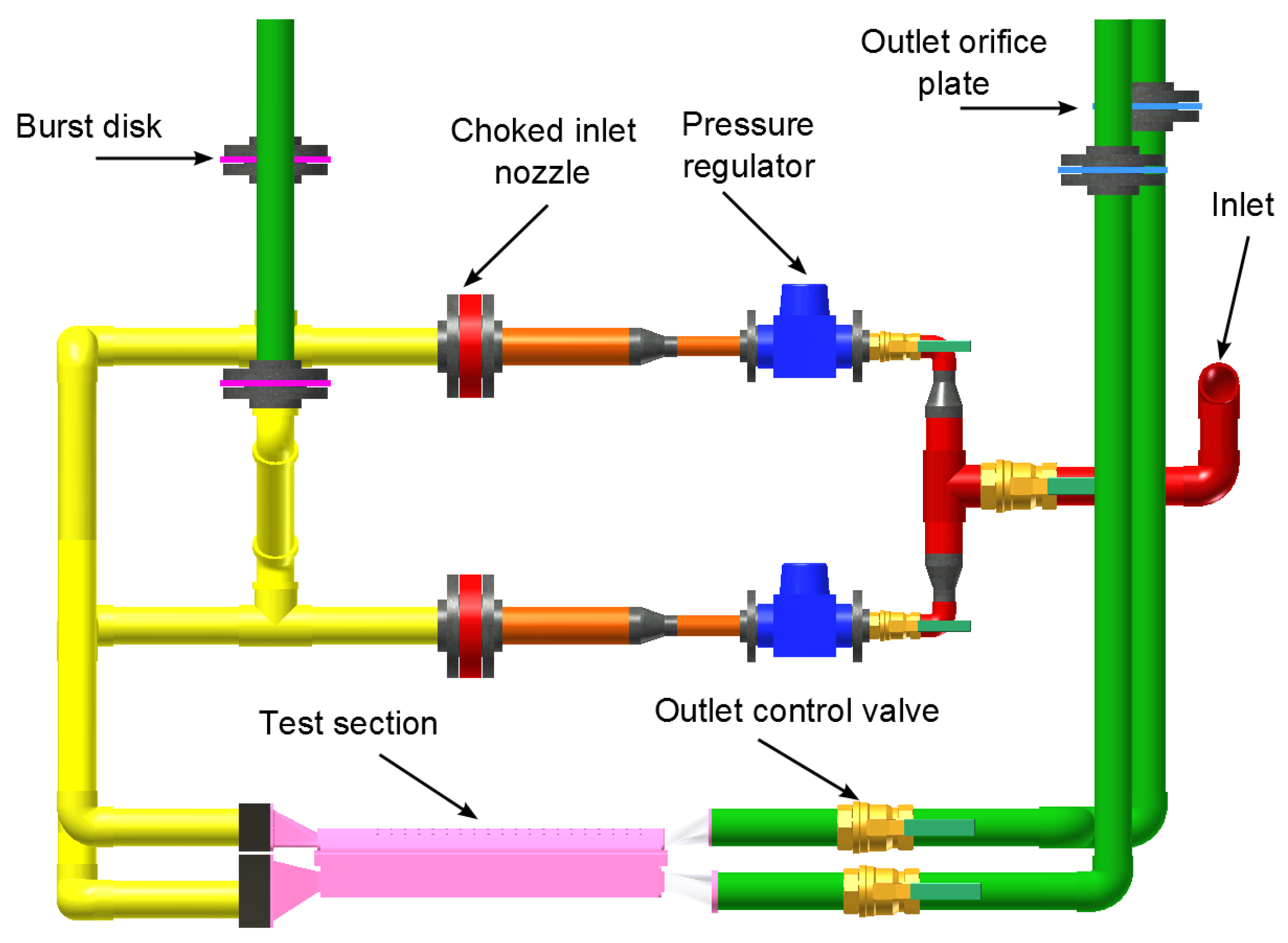
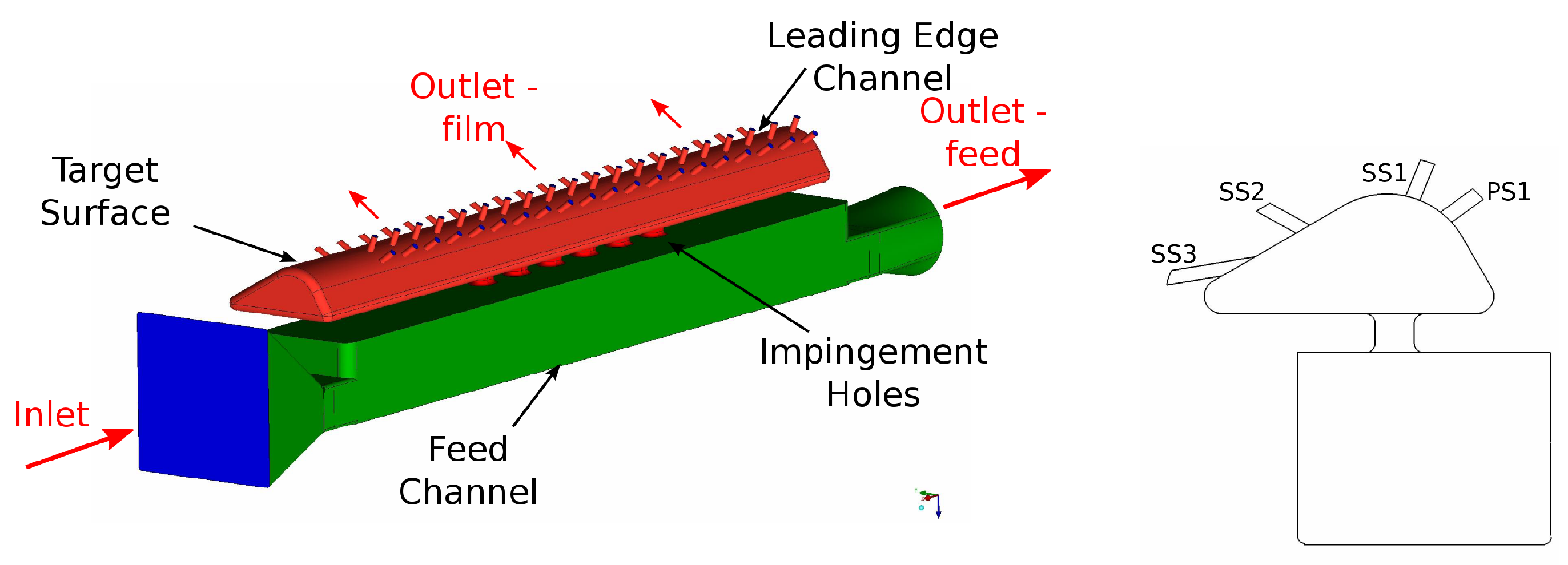
2.1. Overall Rig Design

The experimental setup was designed to provide experimental heat transfer data for a leading edge impingement system under the following conditions:
  • Engine representative jet and passage Reynolds number.
  • Feed passage inlet and outlet flow.
  • Film cooling outlets with engine realistic flow split between different film cooling rows.
  • Multiple different impingement jet geometric configurations
The resulting overall rig layout designed in order to meet these conditions is given in Figure 2.
The rig is supplied with a dry compressed air feed which is maintained at approximately 100 psi (7 bar). The single inlet pipe passes through a ball valve before being split into two separate lines, one each for the feed and leading edge passage, which can both be individually shut off using ball valves. The pipes then pass through similar series of an adjustable pressure regulator and choked venturi nozzle, downstream of which there is an offtake pipe with a burst disk. This is set to a pressure level and with a large enough pipe such that it will burst and exhaust the air before a pressure is reached that can damage the perspex test section. Upstream of the test section there are transition pieces and a heater mesh in order to heat the inlet flow for the transient liquid crystal method. Downstream of the test section, each of the feed and leading edge passage outlets pass through gate valves which are used to control the outlet mass flow rates, which are measured by the orifice plates before being exhausted to atmosphere. The film holes exit directly to atmosphere from the test section.
For the tests that have been carried out in this paper there will be no crossflow in either the feed or leading edge passage, and therefore the inlet and outlet of the leading edge passage, and outlet of the feed passage remain blocked. The experimental setup allows test conditions with both leading edge and feed crossflow to be tested in future studies.

2.2. Mass Flow Control

Multiple mass flow rates must be controlled in order to obtain the required impingement jet Reynolds number and cross flow conditions. The inlet mass flow rates are controlled using critical flow venturi nozzles, while the outlet flow rates are measured using orifice plate flow meters and adjusted using the gate valves upstream of them [9,10,11]. The film hole flows exhaust to atmosphere with a representative mass flow split obtained through a choice of the film hole diameters.

2.3. Test Section Design

The test section was derived from a leading edge impingement design which could be suitable for a modern aero-engine. The leading edge channel is a prismatic scaled, simplified profile of the shape typically found in a leading edge impingement system for a HP turbine blade, shown in Figure 3. The feed channel is a rectangular passage with area and aspect ratio to match the radial passage that feeds the leading edge impingement system in the blade. Four rows of film cooling holes exit the leading edge passage, two rows of showerhead holes and two suction surface shoulder rows. Full geometric details are given for the passages in Table 1 and for the film holes in Table 2. The film hole diameters are scaled from those expected in a real engine case, while the lengths result from the thickness of the wall. The test section wall thickness is constant scaled from a representative engine blade wall.
In the real engine case, both the leading edge and feed passage have crossflow, with a portion of the mass flow both entering and leaving the passage through neither the film or impingement holes. The feed channel is typically the first pass of a radial serpentine passage, while the leading edge requires a flow throughout its length to avoid film ingestion and to provide sufficient cooling in the blade root and tip regions. This is possible to achieve with this rig, however, only conditions with no crossflow in either passage will be considered in the present paper.
The impingement plates are interchangeable in order to allow many different jet configurations to be tested. These will be described in greater detail subsequently in Section 2.6.1.

2.4. Instrumentation

Instrumentation of the experimental setup consists of several pressure and thermocouple measurements, and a video camera for use in obtaining heat transfer measurements. There are thermocouples on the target surface in order for in situ calibration of the thermochromic liquid crystals to be undertaken, and along the centreline of the feed channel to provide a gas reference temperature for the heat transfer calculations.
Pressure and thermocouple measurements were acquired using a National Instruments cDAQ-9174 chassis (National Instruments, Austin, TX, USA) with relevant modules. Labview (National Instruments, Austin, TX, USA) was used to record the data, and monitor mass flow rates, rig temperatures and pressures during the test runs. The final mass flow rates and Reynolds numbers were calculated using the full recorded data processed in Matlab (MathWorks, Natick, MA, USA).

2.5. Heat Transfer Measurement

The heat transfer measurements were obtained using the transient liquid crystal method. The method relies on a solution of the one-dimensional conduction equation to a step change in external gas temperature. The one dimensional heat equation has an analytical solution to this, Equation (1), from which a heat transfer coefficient can be calculated.
T w a l l T i n i t i a l T g a s T i n i t a l = 1 e ( h t ρ c k ) 2 e r f c ( h t ρ c k )
This method requires a step increase in gas temperature for the thermochromic crystals to be activated, which then give information on the surface temperature history of the target surface. Using this temperature history combined with the driving gas temperature the heat transfer coefficients can then be calculated [12]. A video camera is also required to record the colour changes which are then analysed to obtain heat transfer coefficients.
The heater mesh, which provides the increase in gas temperature, consists of a fine mesh connected by conductive busbars and clamped between electrically insulating material. A high current direct current power supply is used to power the mesh.
A camcorder (Panasonic, Kadoma, Japan) was used to to record the video which was then clipped around the relevant test time, and cropped to the region on which the heat transfer coefficients are calculated. The camera is positioned above the test section to give an unobstructed view of the leading edge target surface.
To calculate the Nusselt numbers the THTAC (Transient Heat Transfer Analysis Code) software was used. This software has been developed in house at the Osney Heat Transfer Laboratory for the calculating heat transfer distributions for transient liquid crystal experiments, and has been validated extensively through use in work such as that presented in [12,13,14,15].
The overall uncertainty level for the experimental heat transfer results is approximately 10.0% with the greatest contribution from the uncertainty for the thermal product of perspex.

2.6. Test Conditions

Multiple impingement plate geometries have been tested at different Reynolds number and crossflow conditions, which are detailed in the following sections.

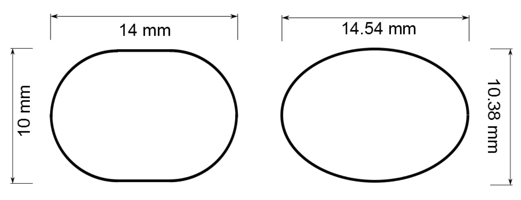
2.6.1. Impingement Geometries

Four different impingement geometries have been tested, with geometric and impingement hole details given in Table 3 and Figure 4.
Each plate comprises either of a single row of holes, or a staggered arrangement. The staggered arrangement consists of two holes in a straight line, followed by four holes offset from this centreline in an alternating manner by distances specified in Table 3. The baseline impingement hole is a racetrack shape, with the elliptical hole specified to have the same hydraulic diameter and cross-sectional area as the racetrack hole. The z / D H for all geometries is 2.55, based on the centreline of the first impingement hole in each case, and each hole has a fillet at its entrance and exit of 2.5 mm.
The staggered and elliptical configurations are being tested as they can offer a reduction in the stresses around the impingement holes in the web region of a turbine blade; however, the use of non-circular holes is only permissible if heat transfer coefficient levels on the target surface are not compromised.

2.6.2. Flow Conditions

Each impingement plate geometry is tested under a range of jet Reynolds numbers from 13,000 to 22,000 to match the lower range expected for engine operation of a similar system.

3. Computational Setup

The setup for the CFD simulations that are compared to the experimental results is given in this section.
Meshing was undertaken using the ICEM 14.0 software (Ansys, Inc., Canonsburg, PA, USA). An unstructured tetrahedral mesh was used with prismatic layers used to capture the boundary layer. Table 4 gives the details for the mesh for the baseline geometry and mid Reynolds number operating condition. The mesh included refinement within the impingement jet region, and y + values remained below 0.5 across the entire impingement target surface.
ANSYS Fluent 14.0 (Ansys, Inc.) was used for all CFD simulations. A stepped solution procedure was followed with the complexity of the calculations built up gradually. The working fluid was air, modelled as an ideal gas with temperature dependent specific heat, viscosity and thermal conductivity. The SIMPLE pressure-based solver was used with second order discretisation for energy, momentum and turbulence properties. The k- ω SST turbulence model was used on account of its accuracy as reported in previous impingement studies [7]. The solver boundary conditions were static pressure at the outlets and prescribed mass flow at the inlet to match experimental conditions. The walls were set to be isothermal at 300 K and the inlet set to 330 K in order to be representative of the experimental setup.
Heat transfer coefficients were calculated for the CFD setup using Equation (2) where T g a s is taken from the same location as the first thermocouple in the feed passage which allows for direct comparisons to the experimental results. Following the calculation of heat transfer coefficients these were converted to Nusselt number, Equation (3), using Sutherland’s law to calculate the temperature dependent thermal conductivity based on the measured centreline gas temperature.
h = q T g a s T w a l l
N u = h D H k

4. Results and Discussion

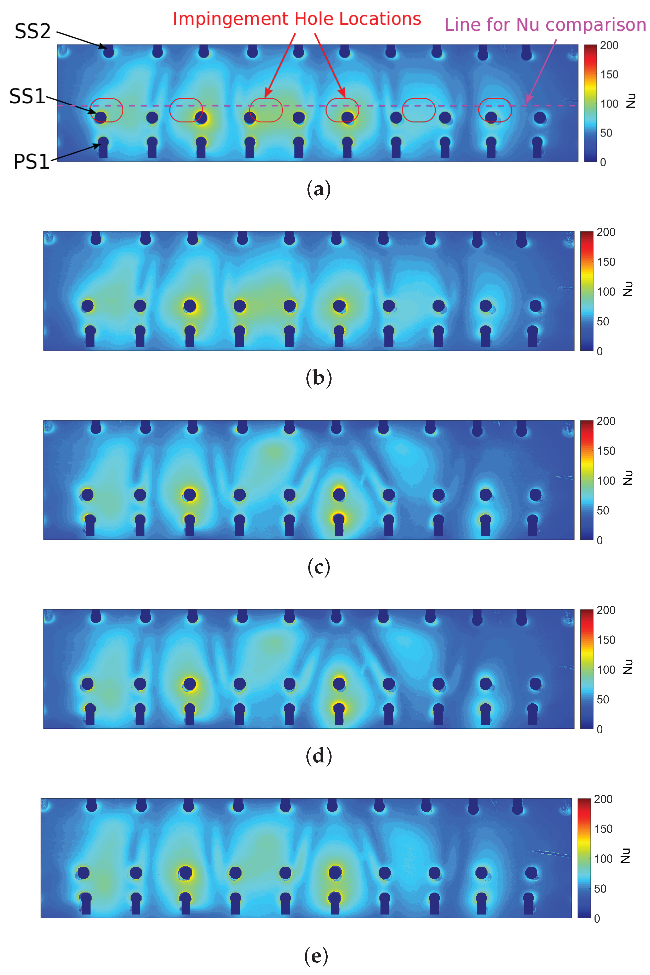
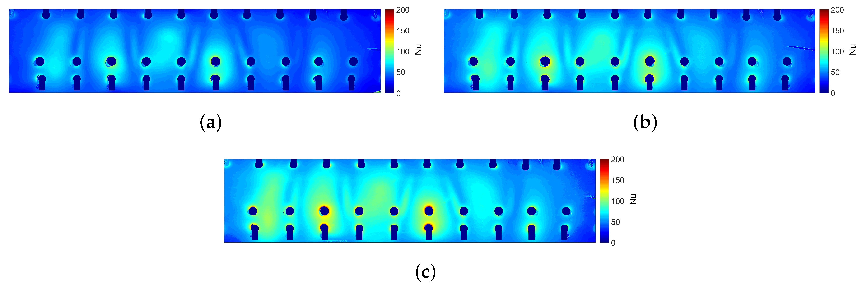
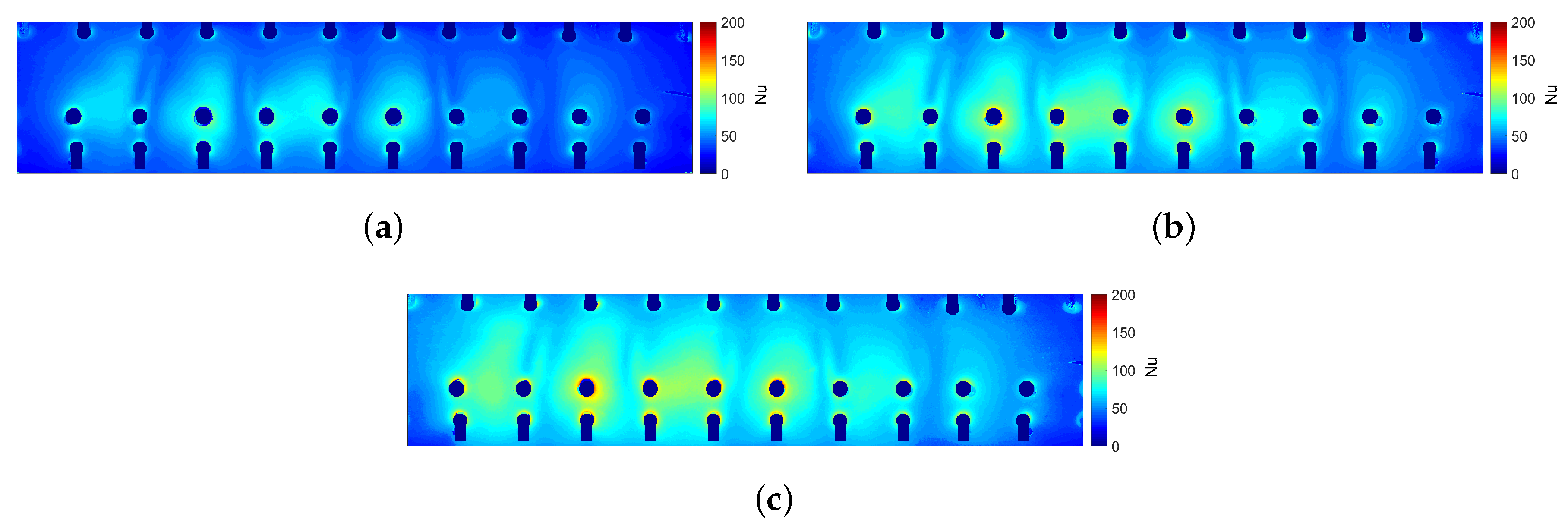
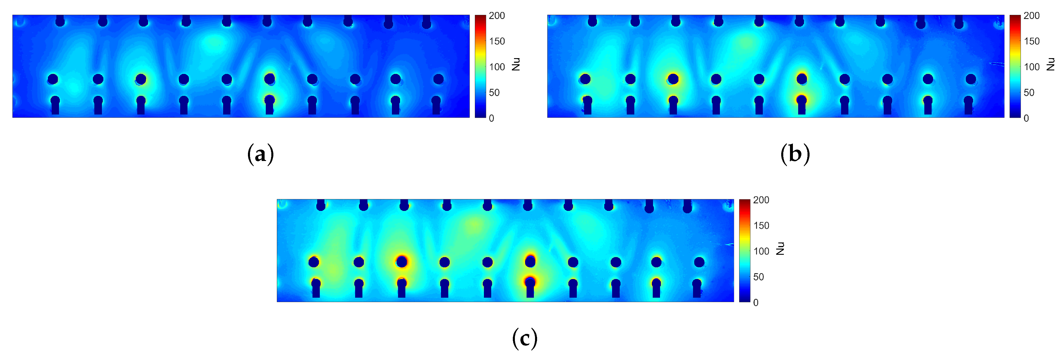
4.1. Experimental Results

Experimental heat transfer results are presented in the form of Nusselt number maps. The THTAC software generates heat transfer coefficient maps for the selected surface, which have then been converted to Nusselt number based on jet hydraulic diameter and temperature dependent gas thermal conductivity. The driving gas temperature for the heat transfer coefficient calculation was chosen to be the first thermocouple in the feed passage, as this is in a region with very small temperature gradients, allowing for an easier comparison to CFD simulations. Areas where the film hole outlets obscured the view of the target surface have been masked out. The film holes that have been masked are the PS1, SS1 and SS2 holes, with the PS1 holes closest to the bottom of the figures. The impingement jets are situated underneath the SS1 films holes, as seen in Figure 3.
Figure 5 shows the Nusselt number maps for each of the four tested geometries for the middle jet Reynolds number of 17,500. The first figure shows a Nusselt map with the film holes labelled, and red shapes to show where the impingement jets are located in the geometry relative to the target surface.
For the first geometry, the peaks of high heat transfer occur in a straight line under each impingement jet, with the third peak from the left giving the highest Nusselt number. The fifth and sixth jets, furthest from the inlet in the feed passage, show significantly reduced levels of heat transfer. This is due to the combination of a reduced flow rate through the jet and by a decrease in the temperature difference between the impinging flow and the wall, and will be explained in greater detail in Section 4.2. There are ridges of high heat transfer between the impingement jets that spread laterally across the leading edge passage. These occur as the flow recirculating from the impinging jets are funnelled across the leading edge geometry towards the SS2 and SS3 film holes, and are investigated further in Section 4.2 where more detail of the internal flow structure can be visualised. Regions of high heat transfer are also found at the entrance to the film holes as flow is accelerated into them, which has previously been observed in [16].
The second geometry shows very similar levels of overall heat transfer; however, with the regions of high heat transfer shifted due to the staggered nature of the impingement hole configuration. The streaks of high heat transfer due to jet interaction are again seen. However, are now angled due to the differing jet locations.
The heat transfer for the third impingement configuration is almost indiscernable from that for the second geometry, indicating that the change from racetrack to elliptical holes has very little impact on the heat transfer distribution. The fourth geometry gives a very similar pattern to the second, the only difference being the location of the staggered jet peaks, which are closer to the single line due to the reduced stagger.
Figure 6, Figure 7, Figure 8 and Figure 9 show the Nusselt number maps for the different impingement geometries for the three Reynolds numbers tested.
For all geometries the overall heat transfer pattern is unchanged, with peaks under the jets and in regions of jet interaction, however with significantly increasing heat transfer with Reynolds number as is expected. This relationship is quantified below in Section 4.3.
Figure 10 shows the experimental Nusselt number along the line shown in Figure 5a for geometries 1 and 2, for the three Reynolds numbers tested. These plots show some of the key features as described previously. The peaks are seen under the impingement jets, and for the streaks of high heat transfer between the jets, which are explained later in this paper. Geometry 1 shows the high peaks of heat transfer for the first four jets, with reduced levels for the fifth and sixth jets. Geometry 2 has very similar Nusselt number levels for the first two jets, with more variable levels for the later jets due to the staggered nature of this configuration. For both geometries the clear increase in heat transfer with Reynolds number is observed.

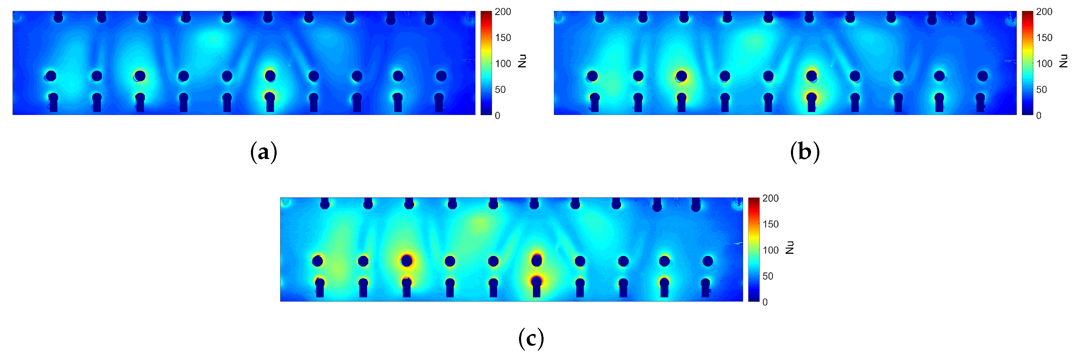
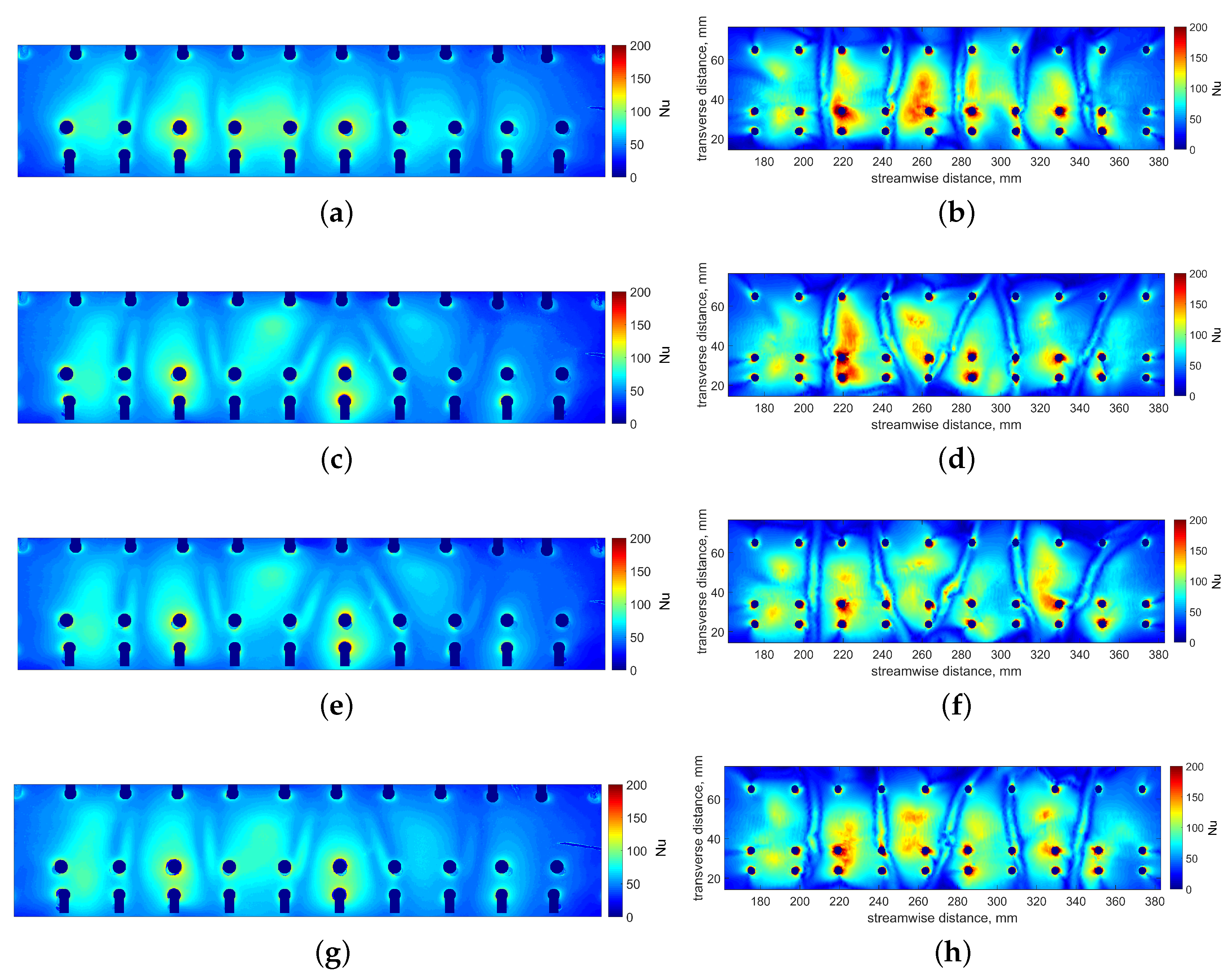
4.2. Comparison of Experimental Results with CFD

Figure 11 shows a comparison between the experimental and CFD results for all geometries at the middle Reynolds number of 17,500. The overall heat transfer distribution is reasonably well predicted, however there are some large differences between the simulations and experimental results.
The location of the peaks of high heat transfer under the impinging jets are predicted well for all geometries, as are the regions of high heat transfer at the entrance to the film holes and between the jets. However, the CFD simulations predict significantly higher peak values and more clearly defined peaks with levels falling away to lower levels away from the jets. The experimental results show less pronounced peaks which spread further across the target surface. This is also found in other studies such as [5].
In both the experimental and CFD results, and across all geometries, a significant decrease in heat transfer is found for the fifth and sixth jets. This results from a combination of both a reduction in flow through these impingement holes and by a decrease in the difference between the temperature of the impinging jet and target wall relative to the previous jets. This is illustrated in Figure 12, which shows the CFD temperature distribution on a plane through the centreline of the impingement jets.
Figure 13 shows a small region of the experimental Nusselt number map for geometry 1 at a Reynolds number of 17,500, in order to highlight the region of high heat transfer streaks between the impingement jets, and a velocity contour with overlayed vectors for a near wall plane for the same region. It can be seen from this that the thin high heat transfer regions results from a high velocity wall jet, that occurs between the impingement jets as the recirculating flow is directed across the leading edge surface. The thin developing boundary layer of the this jet results in a high heat transfer level. These high velocity regions occurs as a combination of the passage shape, that funnels flow in this direction, and also due to the presence of film holes that bleed flow from this passage a distance away from where the jets impinge.

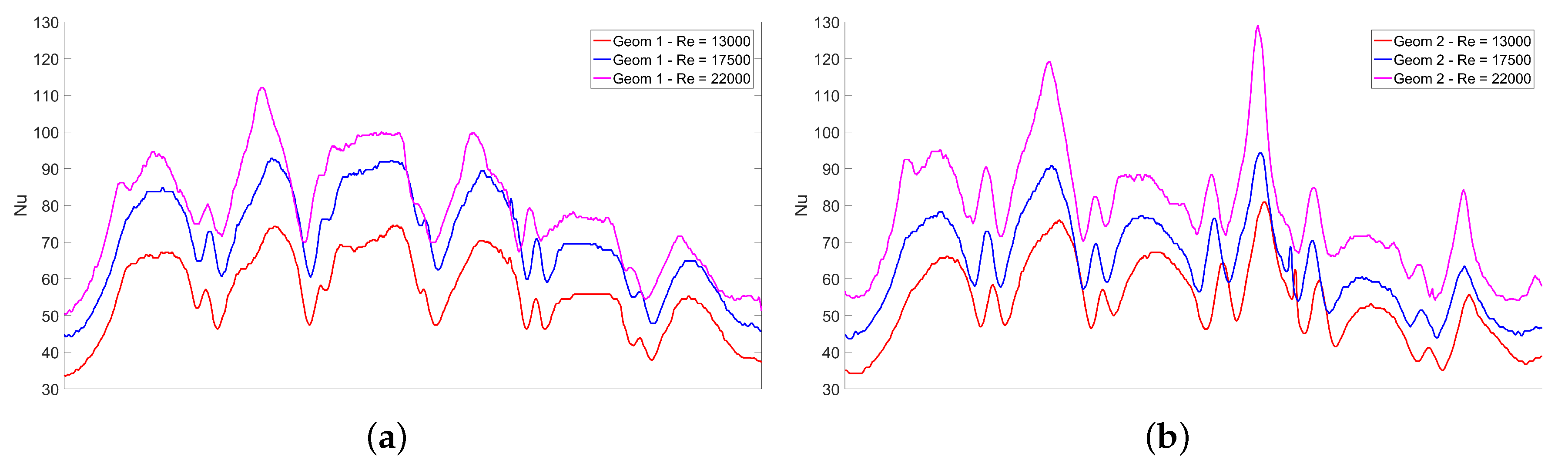
4.3. Heat Transfer—Averages

The Nusselt number maps presented previously have been averaged and plotted below to illustrate the overall heat transfer with varying Reynolds number, Figure 14. The Nusselt number is averaged over the full area presented previously in Figure 5, Figure 6, Figure 7, Figure 8 and Figure 9.
It can be clearly seen that the impingement hole configuration has little effect on heat transfer. For both the experimental and CFD results the overall heat transfer levels are similar for all geometries for a given Reynolds number. This is an important result for thermal engineers who may use the staggered configuration, or elliptical jets, in order to reduce stress concerns in the web region where the impingement holes are placed, which can be done without reducing the leading edge heat transfer.
The CFD consistently overpredicts the heat transfer for this system by approximately 10% across all geometries and Reynolds numbers.
A power fit of the form a R e b has been produced for the experimental data, given in Equation (4) and illustrated on Figure 14. The other correlation shown on Figure 14 is that for the most similar geometry found in [7], and shows good agreement with the experimental data, albeit with a slightly different relationship with Reynolds number. The experimental data is also in line with other relationships for impingement systems found in the literature such as [5,6]. The levels produced from these other correlations are around 8% higher that those found in a similar leading edge system in [5], with this difference put down to the lower z / D H and asymmetric leading edge passage shape found in this work. The Reynolds exponent of approximately 0.71 is similar to that of many previous impingement correlations, for example those presented in [7,8,17,18]. The overall Nusselt number levels do show some difference to these previous studies due to varying driving gas temperature definitions and the asymmetric nature of the leading edge passage in this study.
N u = 0.05738 R e 0.7093

5. Conclusions

A new experimental rig for a leading edge impingement system has been designed and constructed, and a series of heat transfer tests have been completed. Four different impingement configurations have been tested for an engine-representative HP turbine blade leading edge geometry with film cooling rows. The heat transfer distributions and levels have been compared to RANS CFD simulations.
The following conclusions have been drawn:
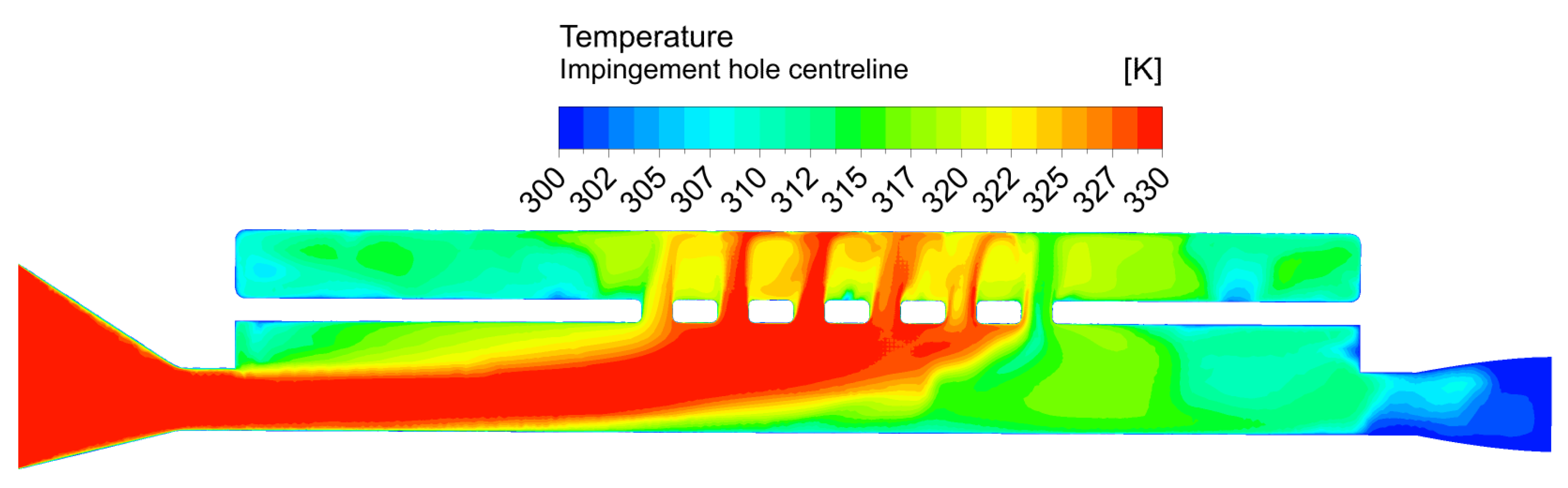
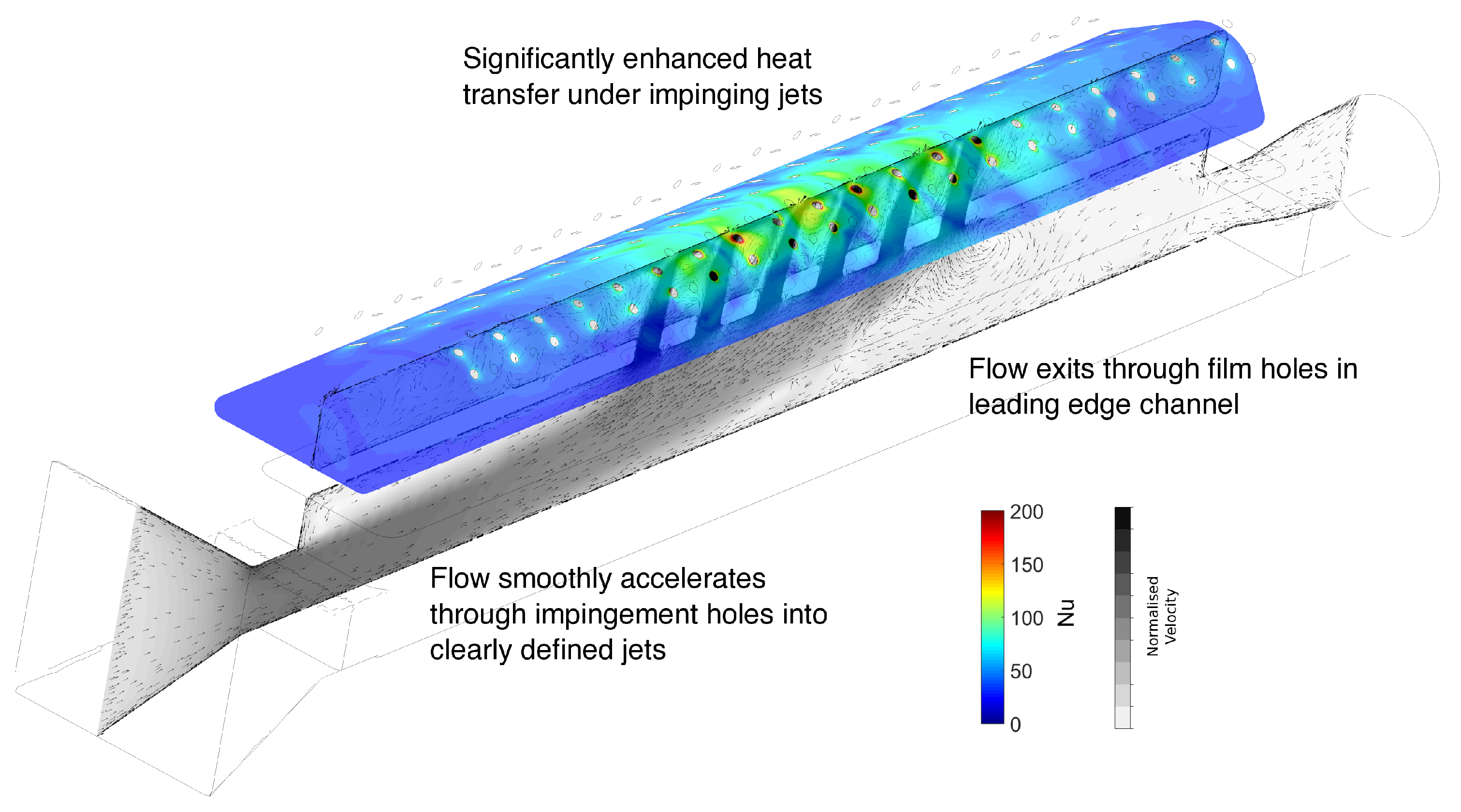
  • The experimental heat transfer distributions produced show the typical patterns expected of such a system, with peaks of high heat transfer under each impinging jet.
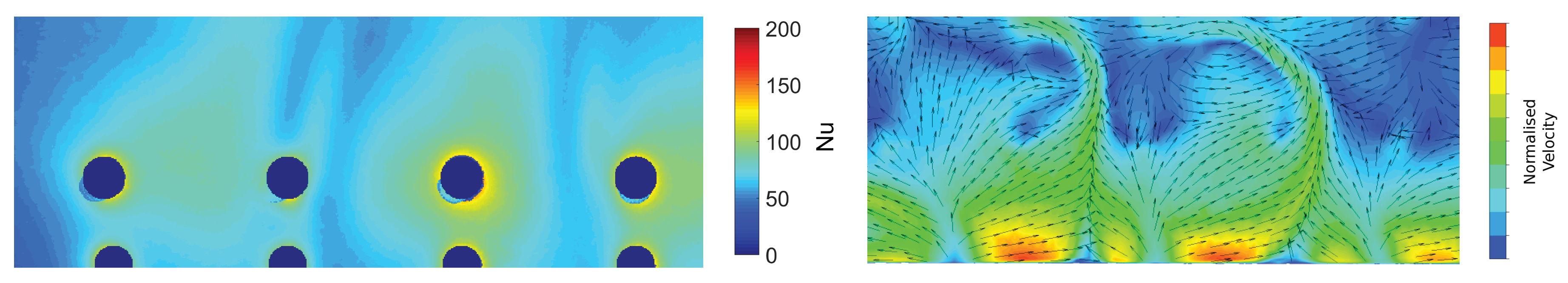
  • Additional regions of high heat transfer are also seen where flow accelerates into the film cooling holes, and between the jets where recirculating, high velocity flow is funnelled across the leading edge surface towards the suction surface film cooling holes.
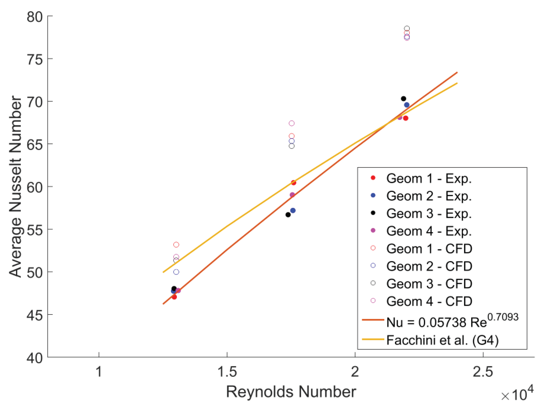
  • The effect of altering the impingement configurations on heat transfer is very small, which allows the rearrangement of jets to such configurations to reduce web stresses in a turbine blade.
  • An increase in jet Reynolds number gives an increased surface Nusselt number in line with previous studies.
  • CFD simulations reasonably predict the overall heat transfer distribution, with a consistent overprediction in levels of approximately 10%.

Author Contributions

All authors conceived and designed the experimental test rig and defined the experimental conditions; Robert Pearce performed the experiments, analysed the data and wrote the paper.

Funding

This work was funded by Rolls-Royce plc.

Acknowledgments

Experimental support was provided by James Turner and the workshop at the Osney Thermofluids Institute.

Conflicts of Interest

The authors declare no conflicts of interest.

Abbreviations

The following abbreviations are used in this manuscript:
AArea
cSpecific Heat
CFDComputational Fluid Dynamics
DDiameter
D H Hydraulic Diameter
hHeat Transfer Coefficient
HPHigh Pressure
kThermal Conductivity
L f Length of Film Hole
L p Length of Passage
LELeading Edge
NuNusselt Number
pPitch
qHeat Flux
RANSReynolds-averaged Navier-Stokes
R e Reynolds Number
tTime
T i n i t i a l Initial Temperature
T g a s Gas Temperature
T w a l l Wall Temperature
zJet-target distance
ρ Density

References

  1. Zuckerman, N.; Lior, N. Jet impingement heat transfer: Physics, correlations, and numerical modelling. Adv. Heat Transf. 2006, 39, 565–631. [Google Scholar]
  2. Son, C.; Gillespie, D.; Ireland, P.; Dailey, G. Heat transfer characteristics of an impingement plate used in a turbine vane cooling system. In Proceedings of the ASME Turbo Expo 2001: Power for Land, Sea, and Air, New Orleans, LA, USA, 4–7 June 2001. 2001-GT-0154. [Google Scholar]
  3. O’Donovan, T.; Murray, D. Jet impingement heat transfer—Part I: Mean and root-mean-square heat transfer and velocity distributions. Int. J. Heat Mass Transf. 2007, 50, 3291–3301. [Google Scholar] [CrossRef]
  4. O’Donovan, T.; Murray, D. Jet impingement heat transfer—Part II: A temporal investigation of heat transfer and local fluid velocities. Int. J. Heat Mass Transf. 2007, 50, 3302–3314. [Google Scholar] [CrossRef]
  5. Facchini, B.; Maiuolo, F.; Tarchi, L.; Ohlendorf, N. Experimental Investigation on the Heat Transfer of a Leading Edge Cooling System: Effects of jet-to-jet spacing and showerhead extraction. In Proceedings of the ASME Turbo Expo 2013: Turbine Technical Conference and Exposition, San Antonio, TX, USA, 3–7 June 2013. GT2013-94759. [Google Scholar]
  6. Facchini, B.; Maiuolo, F.; Tarchi, L.; Ohlendorf, N. Experimental Investigation on the Heat Transfer in a Turbine Airfoil Leading Edge Region: Effects of the Wedge Angle and Jet Impingement Geometries. In Proceedings of the 10th European Conference on Turbomachinery, Fluid Dynamics and Thermodynamics, Lappeenranta, Finland, 15–19 April 2013. ETC2013-130. [Google Scholar]
  7. Facchini, B.; Maiuolo, F.; Tarchi, L.; (University of Florence, Florence, Italy). D2.4 Report on UNIFI experiments. EU FP7 ERICKA Technical Report. 2013. [Google Scholar]
  8. Chupp, R.; Helms, H.; McFadden, P.W. Evaluation of internal heat transfer coefficients for impingement cooled turbine airfoils. J. Aircr. 1969, 6, 203–208. [Google Scholar]
  9. ISO. BS EN ISO 9300:2005—Measurement of Gas Flow by Means of Critical Flow Venturi Nozzles; International Organization for Standardization: Geneva, Switzerland, 2005. [Google Scholar]
  10. ISO. BS EN ISO 5167-2:2003—Measurement of Fluid Flow by Means of Pressure Differential Devices Inserted in Circular-Cross Section Conduits Running Full—Part 2; International Organization for Standardization: Geneva, Switzerland, 2003. [Google Scholar]
  11. ISO. BS EN ISO 5167-1:2003—Measurement of Fluid Flow by Means of Pressure Differential Devices Inserted in Circular Cross-Section Conduits Running Full—Part 1; International Organization for Standardization: Geneva, Switzerland, 2003. [Google Scholar]
  12. Ryley, J. Turbine Blade Mid-Chord Internal Cooling. Ph.D. Thesis, University of Oxford, Oxford, UK, 2014. [Google Scholar]
  13. McGilvray, M.; Orozco Piñeiro, C.; Axe, T.; Ryley, J.; Gillespie, D. Comparison of stationary internal cooling passage numerical simulations to experimental data. In Proceedings of the 10th European Tubomachinery Conference, Lappeenranta, Finland, 15–19 April 2013. ETC2013-170. [Google Scholar]
  14. Ryley, J.; McGilvray, M.; Gillespie, D. Stationary internal cooling passage experiments for an engine realistic configuration. In Proceedings of the 10th European Conference on Turbomachinery, Fluid Dynamics and Thermodynamics, Lappeenranta, Finland, 15–19 April 2013. [Google Scholar]
  15. McGilvray, M.; Gillespie, D.; Ryley, J. Investigation of wrapping ribs onto smooth walls for mid-chord internal cooling passages. In Proceedings of the ASME Turbo Expo 2014: Turbine Technical Conference and Exposition, Düsseldorf, Germany, 16–20 June 2014. GT2014-26973. [Google Scholar]
  16. Gillespie, D.; Wang, Z.; Ireland, P.; Kohler, S. Full surface local heat transfer coefficient measurements in a model of an integrally cast impingement cooling geometry. J. Turbomach. 1998, 120, 92–99. [Google Scholar] [CrossRef]
  17. Huang, Y.; Ekkad, S.; Han, J. Detailed heat transfer distributions under an array of orthogonal impinging jets. J. Thermophys. Heat Transf. 1998, 12, 73–79. [Google Scholar] [CrossRef]
  18. Romero, E.; (Rolls-Royce plc, Bristol, UK); Tarchi, L.; (University of Florence, Florence, Italy); Bauer, R.; Alstom, Baden, Switzerland. D2.5 Report of Results on Rotating Heat Transfer Tests—Impingement Cooling Geometries. EU FP7 ERICKA Technical Report. 2014. [Google Scholar]
Figure 1. Computational fluid dynamics (CFD) results showing representative flow structure—velocity distributions in grayscale, surface heat flux in colour.
Ijtpp 03 00023 g001
Figure 2. Schematic of experimental setup.
Ijtpp 03 00023 g002
Figure 3. Test section geometry and cross section.
Ijtpp 03 00023 g003
Figure 4. Impingement hole profiles—racetrack and elliptical.
Ijtpp 03 00023 g004
Figure 5. Comparison of measured Nusselt number distributions for all geomtries at R e = 17,500. (a) Figure showing Nu map, with indicative impingement hole locations, and film hole labels; (b) Geometry 1—single line, racetrack; (c) Geometry 2—staggered, racetrack; (d) Geometry 3—staggered, elliptical; (e) Geometry 4—reduced stagger, racetrack.
Ijtpp 03 00023 g005
Figure 6. Comparison of measured Nusselt number distributions for geometry 1 with R e = 13,000, 17,500 and 22,000. (a) R e = 13,000; (b) R e = 17,500; (c) R e = 22,000.
Ijtpp 03 00023 g006
Figure 7. Comparison of measured Nusselt number distributions for geometry 2 with R e = 13,000, 17,500 and 22,000. (a) R e = 13,000; (b) R e = 17,500; (c) R e = 22,000.
Ijtpp 03 00023 g007
Figure 8. Comparison of measured Nusselt number distributions for geometry 3 with R e = 13,000, 17,500 and 22,000. (a) R e = 13,000; (b) R e = 17,500; (c) R e = 22,000.
Ijtpp 03 00023 g008
Figure 9. Comparison of measured Nusselt number distributions for geometry 4 with R e = 13,000, 17,500 and 22,000. (a) R e = 13,000; (b) R e = 17,500; (c) R e = 22,000.
Ijtpp 03 00023 g009
Figure 10. Comparison of measured Nusselt number distributions on line near to impingement peaks for geometries 1 and 2 with R e = 13,000, 17,500 and 22,000. (a) Geometry 1; (b) Geometry 2.
Ijtpp 03 00023 g010
Figure 11. Comparison of measured Nusselt number distributions with CFD predictions for all geometries at R e = 17,500. (a) Geom 1—Exp.; (b) Geom 1—CFD; (c) Geom 2—Exp.; (d) Geom 2—CFD; (e) Geom 3—Exp.; (f) Geom 3—CFD; (g) Geom 4—Exp.; (h) Geom 4—CFD.
Ijtpp 03 00023 g011
Figure 12. CFD temperature distribution on centreline of impingement holes for geometry 1 at R e = 17,000.
Ijtpp 03 00023 g012
Figure 13. Detailed view of measured high heat transfer region between jets (experimental Nusselt number) with CFD near-wall velocity contour for the same region.
Ijtpp 03 00023 g013
Figure 14. Heat transfer averages—comparison between experiment and CFD simulations.
Ijtpp 03 00023 g014
Table 1. Geometric details—passages.
FeedLeading Edge
D H  (mm)55.936.1
A (mm 2 )31851582
L p  (mm)500500
Table 2. Geometric details—film cooling.
PS1SS1SS2SS3
No. Rows20202020
D (mm)3.53.53.83.8
L f  (mm)9.69.410.313.3
p (mm)20202020
Table 3. Impingement geometry details.
Geom.Jet No.Hole ShapeArrangementHole D h (mm)Hole Area (mm 2 )
16RacetrackSingle line 12.0 118.5
26RacetrackStaggered— 7.5  mm 12.0 118.5
36EllipticalStaggered— 7.5  mm 12.0 118.5
46RacetrackStaggered— 3.75  mm 12.0 118.5
Table 4. Mesh details for CFD simulations.
No. of CellsNo. of Prism LayersMax y + Area-Averaged y +
11.6 million152.1570.269

