Analysis of Interactions Among Loss-Generating Mechanisms in Axial Flow Turbines ^†

Abstract

Accurate loss prediction since the preliminary design steps is crucial to improve the development process and the aerodynamic performance of turbines. Initial design phases typically employ reduced-order models in which the different loss-generating mechanisms are assessed through correlations. These correlations are often based on the hypothesis of loss linearity, which assumes that losses from different sources can be summed to obtain the total losses. However, this assumption could constitute an oversimplification, as losses occur concurrently and can interact with each other, potentially impacting overall performance, all the more in low aspect ratio turbomachinery. The aim of this paper is to investigate the role of interactions between different phenomena in the generation of loss. 3D RANS simulations are run on two simplified representations of a turbine blade channel, a curved duct and a linear cascade, and on a real turbine vane. Several inlet and wall boundary conditions are employed to examine loss-generating phenomena both separately and simultaneously. This approach enables the analysis of where and how interactions occur and quantifies their influence on the overall losses. Losses caused by boundary layer–vortex interactions are found to be highly sensitive to the relative positions of these two phenomena. It was observed that the loss linearity assumption may be acceptable in certain cases, but it is generally inadequate for off-design conditions and twisted annular configurations.

1. Introduction

Early assessment of turbine flow losses is critical for a fast and accurate turbine design process. A thorough understanding of the various phenomena generating loss in the flow can assist in accurately estimating and containing such loss. The sooner this is achieved, the smoother and more cost-effective the design process will be.

At present, early design phases rely on reduced-order models, which predict losses through correlations. According to Aungier [1], among the best-documented and most widely employed correlations are those from Ainley and Mathieson [2]—later improved by Dunhame and Came [3] and Kacker and Okapuu [4]—and those introduced by Stewart [5] and by Craig and Cox [6]. More recent work by Moustapha et al. [7] and Benner et al. [8] involves the modeling of off-design conditions. Many other models are summarized in [9,10], including those of Soderberg [11], Traupel [12], and Zehner [13]. As pointed out by Denton [14], these correlations are not fully representative of what physically occurs in turbine flows, as they frequently derive from experimental data collected several decades ago on a limited number of cascade and turbine geometries. Moreover, these models sometimes apply to both gas and steam turbines, making them less specific. Efforts are occasionally made to obtain loss models analytically [5,15], but they still rely on strong and oversimplified assumptions. While some authors propose corrections for the Mach number [3,4,6,16], many applications are restricted to subsonic flows, with the precise validity range often left unspecified by the authors. Such limitation poses an issue as transonic turbines become increasingly common to reduce the total number of stages. Moreover, constraints in terms of geometrical parameters do not reflect recent turbine blade shapes, especially in high-pressure turbines where blades are nowadays thicker due to cooling requirements.

In all these correlations, the various loss sources are modeled independently, and they are usually categorized as follows:

• Profile loss: It is the loss generated by the blade boundary layers. The flow is assumed to be two-dimensional, meaning that the blade boundary layer is considered far from the endwalls.
• Endwall (or secondary) loss: it takes into account the loss generated by the hub and shroud boundary layers (although the portions of the endwalls before the leading edge and after the trailing edge are often neglected) and by the secondary flows that can originate at the corners where the blade meets the endwalls.
• Tip clearance loss: sometimes considered as part of the endwall loss, it is caused by the passage of the leakage flows across the clearance, which leads to an energy loss due to the reduced working mass flow and a change in the exit flow direction.
• Trailing edge loss: It represents the mixing loss downstream of the trailing edge (TE). Few models consider it as an independent loss source [4,5], while in most cases, it is obtained from profile and endwall losses through a multiplying factor [2,3,6].

The total losses in a turbine row are obtained by summing the above contributions under the hypothesis of loss linearity. This is an important assumption since it is well-established that interactions can occur between loss-generating phenomena. For instance, vortices arise as the boundary layers from the endwalls interact with the boundary layer of the blade, a phenomenon that is particularly significant when the aspect ratio is low. Besides, high-angle deviation of the blade boundary layer leads to secondary flows, which result in a three-dimensional flow pattern. These phenomena are often overlooked in correlations, which assume that the blade boundary layer is two-dimensional and independent of the endwall losses. However, evaluating the extent to which interactions influence total losses and how the assumption of loss linearity deviates from reality remains challenging.

The present work, which is based on a version previously presented at the 16th European Turbomachinery Conference [17], aims to investigate the presence and the influence of nonlinearity in turbine flows. RANS calculations are run on three different configurations: a curved duct, a linear cascade, and a turbine Nozzle Guide Vane (NGV). Several combinations of inlet and wall boundary conditions are set in an attempt to simulate different loss-generating phenomena both when they occur simultaneously and when they are isolated. Comparisons between the different simulations are performed, enabling us to analyze where and how interactions occur and to quantify their influence on the overall losses. The purpose is to determine whether the loss breakdown used in correlations yields reasonable results despite the strong underlying assumptions and, if this is not the case, to identify ways to improve it.

The following section describes the configurations selected for the study. The numerical setup, along with the specific boundary conditions and geometric features of each RANS simulation, is detailed. Section 3 introduces the loss formulation employed, which includes both the loss generated within the domain and the potential loss due to mixing to uniform flow conditions downstream of the domain. Section 4 presents the results of the entropy analysis and comparison between the different RANS simulations. Finally, Section 5 draws some conclusions and future perspectives.

2. Configurations and Numerical Setup

Three geometries were used in this work in an attempt to investigate the interactions between different loss sources in turbine flows. The first geometry is the curved duct shown in Figure 1a. This is a simple configuration, with an initial straight part, followed by a curve and a reduction in the cross-section, which results in a flow deviation similar to that in a turbine blade passage. As displayed in Figure 2, the side walls are solid walls up to the end of the curve ($\tilde{\mathrm{x}}=1$), then periodicity is set in order to maintain the flow deviation. By injecting swirl components at the inlet of the domain, the curved duct was used to investigate the boundary layer–vortex interaction. The second geometry is a linear cascade (Figure 1b). The blade profile is the mid-span profile of the nozzle guide vane of the FACTOR turbine (FACTOR – Full Aerothermal Combustor Turbine interactiOns Research – is a European research project for the optimization of the interactions between the combustor and the high-pressure turbine [18]). One blade passage is simulated, with periodicity imposed on the lateral walls. The domain length and span are equal to those of the curved duct. Different versions of the linear cascade were created for the scope of this paper, including different span heights to vary the aspect ratio. The third geometry is the NGV of the FACTOR turbine (Figure 1c), which is characterized by a three-dimensional design featuring twisted blades and a varying annulus radius. As for the linear cascade, one blade passage is simulated.

The curved duct configuration was used to study a specific type of interaction—the one between a vortex and a boundary layer. This raised questions about linearity and prompted further investigation into turbine configurations. To address the broader question of whether the hypothesis of loss linearity is acceptable for establishing correlations, the linear cascade and the turbine NGV were employed. In Figure 1, the inlet and outlet post-processing planes are colored in red. For the curved duct, the inlet and outlet plane are located respectively at the real domain inlet ($\tilde{\mathrm{x}}=-2$) and at the end of the curve ($\tilde{\mathrm{x}}=1$). For the linear cascade and the NGV, the two planes are located at a quarter of the axial chord upstream of the leading edge (LE) and downstream of the trailing edge (TE), respectively. All the results presented in this paper pertain to the portion of the two domains between the inlet and the outlet planes. The remaining parts of the two domains were included only to improve the convergence of the simulations.

Both the curved duct and the two-bladed geometries have already been employed within the Aerodynamics and Propulsion department of ISAE-Supaero [19,20,21,22]. The multi-block structured meshes were generated with the IGG/AutoGrid software from Cadence. A grid convergence study was conducted for the curved duct configuration, retaining a mesh of 7.5 million cells, with $y^{+}$ values predominantly below 1 and always below 3. All the numerical simulations were performed with the elsA CFD software (version $3.8$) [23]. elsA is a multi-block cell-centered implicit finite volume solver developed by ONERA. The numerical setup used in this paper is the one employed by Safran Aircraft Engines for RANS simulations in elsA: Jameson’s second-order space discretization scheme [24] and the Wilcox $k-\omega$ turbulence model [25]. The turbulent boundary conditions were set with a turbulence intensity of $4\%$ and a turbulence length scale of 1 mm for all simulations. RANS simulations are widely used in the industry as they offer a valuable compromise: they allow for a large number of runs at a reasonable computational cost and within a manageable time frame while still delivering sufficiently accurate results when it comes to modeling simple turbine geometries and advancing the development of pre-design reduced-order models. This makes them well-suited for the present approach. Moreover, validation of RANS simulations performed using the elsA code on the FACTOR turbine has been thoroughly carried out by Wingel [21], showing good agreement with experimental measurements.

2.1. Curved Duct Simulations

The curved duct was selected as it allows us to analyze the interactions between different wall boundary layers and vortices, as well as their impact on the linearity of losses. Indeed, several simulations were run, and in some cases, vortices were injected at the domain inlet at two different locations. In the context of an axial flow turbine, in which many vortices are present close to the blade and end walls (tip leakage vortex, passage vortex, horseshoe vortex…), this configuration—characterized by the absence of wakes and the known properties of the vortex—helps simplify the blade–endwall interaction and the effects of a passing vortex on the overall losses. The aim of simulating different vortex locations was to investigate how different levels of interaction with the walls can influence the overall loss. This approach allows us to assess how far the separate consideration of secondary and profile losses can deviate from reality.

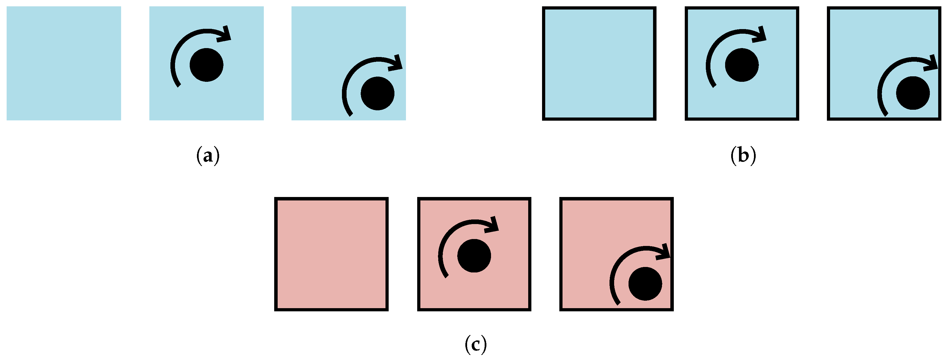
All the simulations that were run on the curved duct domain are represented in Figure 3, which gives a visual representation of the inlet of these simulations. The black contour stands for the wall boundary layer, the black dot is representative of the vortex core radius and location, and the arrow indicates the vortex direction of rotation (when looking at the inlet from a coordinate $\tilde{\mathrm{x}}<-2$). In cases Duct1, Duct2, and Duct3, the four walls were assigned a slip condition. The only loss occurring in case Duct1 is streamwise shear loss due to the flow turning, which includes a curve and a reduction in the cross-section. Cases Duct2 and Duct3 allow quantifying the amount of loss generated by the injected vortices without any vortex–boundary layer interaction taking place. Cases Duct4, Duct5, and Duct6 present the same inlet conditions as the three previous cases, respectively, but a no-slip condition was applied to the walls to add the presence of the boundary layers. Therefore, a comparison of cases Duct4, Duct5, and Duct6 with the previous three cases allow us to quantify the loss generated by boundary layers and the effects of interactions with a vortex positioned at two different locations. Finally, in cases Duct7, Duct8, and Duct9, the outlet pressure was lowered to accelerate the flow to supersonic conditions: these simulations helped assess the impact of flow velocity on boundary layer and vortex losses, as well as on their interaction.

The Reynolds number (in the curved duct, the Reynolds number was calculated at $\tilde{\mathrm{x}}=-2$ using the mean curvature line as characteristic length.) is approximately equal to $2.70·{10}^5$ for cases Duct1 to Duct6 and to $2.85·{10}^5$ for cases Duct7 to Duct9. Uniform total pressure and total temperature values were set as inlet boundary conditions in the absence of injected vortices, with axial flow velocity direction. In all cases presenting a vortex, Vatistas’ vortex generation model [26] was used for the inlet boundary conditions. This model defines the tangential velocity $v_{\theta }$ as a function of the radius from the vortex center:

$$v_{\theta }\left(r\right)={\displaystyle \frac{\mathrm{\Gamma }}{2\pi }}\left[{\displaystyle \frac{r}{r_c^2+r^2}}\right]$$

(1)

Since here, pressure and temperature inlet boundary conditions were used, only the velocity direction was imposed in terms of $v_{\theta }/v_{\infty }$. The pressure field was derived from the radial equilibrium equation and reads:

$$P_s=P_{\infty }-{\displaystyle \frac{\rho }{2}}{\left[{\displaystyle \frac{\mathrm{\Gamma }}{2\pi r_c}}\right]}^2\left[{\displaystyle \frac{r_c^2}{r_c^2+r^2}}\right]$$

(2)

The vortex core radius $r_c$ was set to $1/8$ of the inlet side length, and a circulation $\mathrm{\Gamma }=2{\mathrm{m}}^2{\mathrm{s}}^{-1}$ was imposed for all injected vortices. The vortex center was set either at the inlet center or at $1/4$ span from the right and bottom walls. For each triplet of cases, the outlet pressure was adjusted to achieve a consistent mass flow rate (see

Table 1. List of curved duct simulations.

Case	$\widetilde{\dot{\mathbf{m}}}$	VIC $(\tilde{\mathbf{x}},\tilde{\mathbf{y}},\tilde{\mathbf{z}})$	Wall BC
Duct1	1	-	slip
Duct2	1	(0, 1/2, 1/2)	slip
Duct3	1	(0, 1/4, 1/4)	slip
Duct4	1	-	no-slip
Duct5	1	(0, 1/2, 1/2)	no-slip
Duct6	1	(0, 1/4, 1/4)	no-slip
Duct7	1.032	-	no-slip
Duct8	1.032	(0, 1/2, 1/2)	no-slip
Duct9	1.032	(0, 1/4, 1/4)	no-slip

) in order to allow for a comparison of the total losses and an evaluation of the effect of interactions.

The normalized mass flow rate, the vortex inlet coordinates $(x,y,z)$ normalized by the duct span (VIC) and the wall boundary conditions (BC) of all curved duct simulations are summarized in Table 1.

2.2. Linear Cascade and Turbine NGV Simulations

As mentioned in the introduction, the two-loss categories that are present in every correlation are profile loss and endwall loss, which sometimes also include vortices and secondary flows that form close to the blade–endwall corners (tip clearance and TE losses are often included in the first two categories or obtained through multiplying factors). The profile loss is a two-dimensional loss, so it does not take into account the interaction of the blade boundary layer with the endwall boundary layers. The endwall loss is simply summed to the profile loss to obtain the total loss.

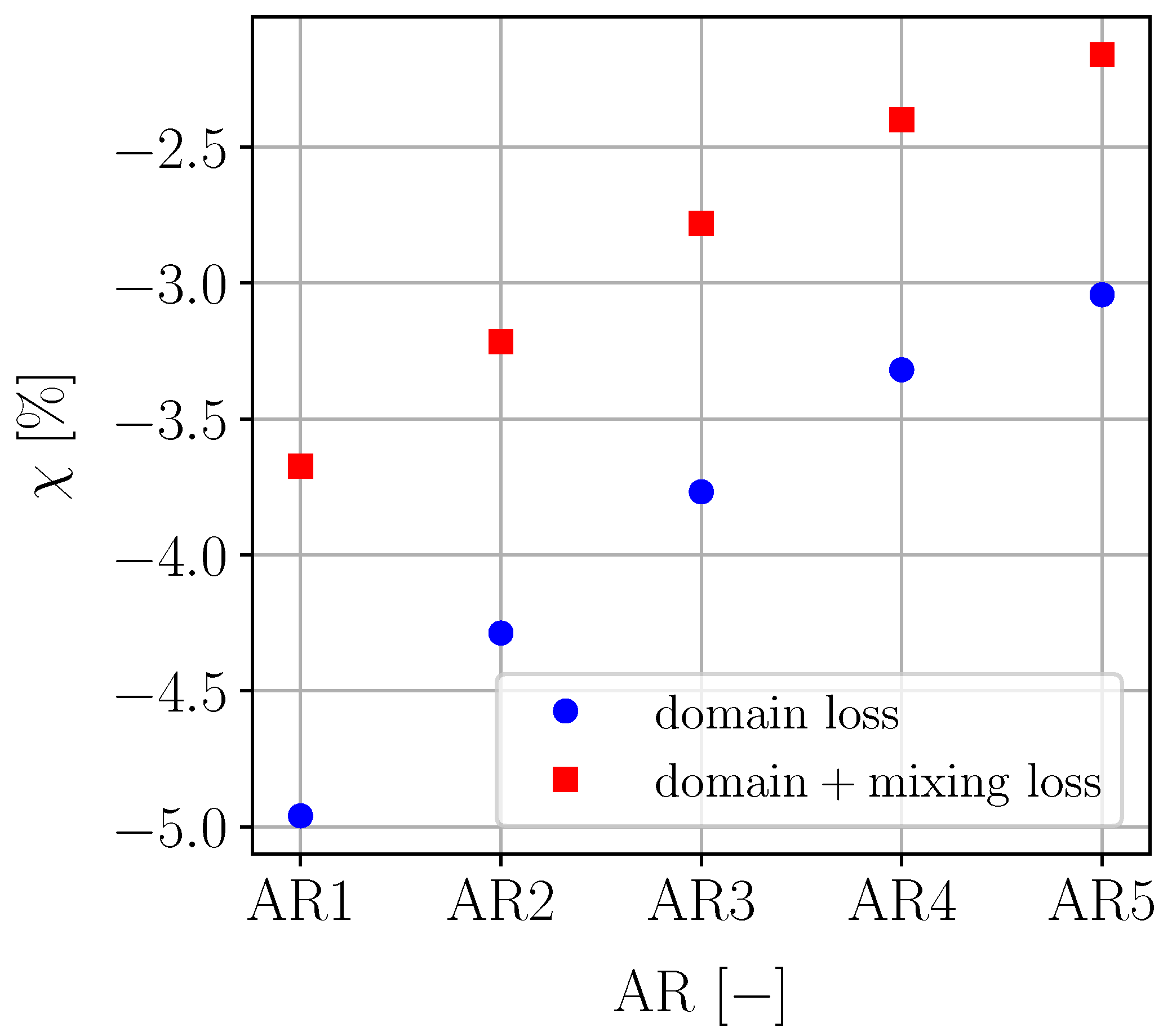
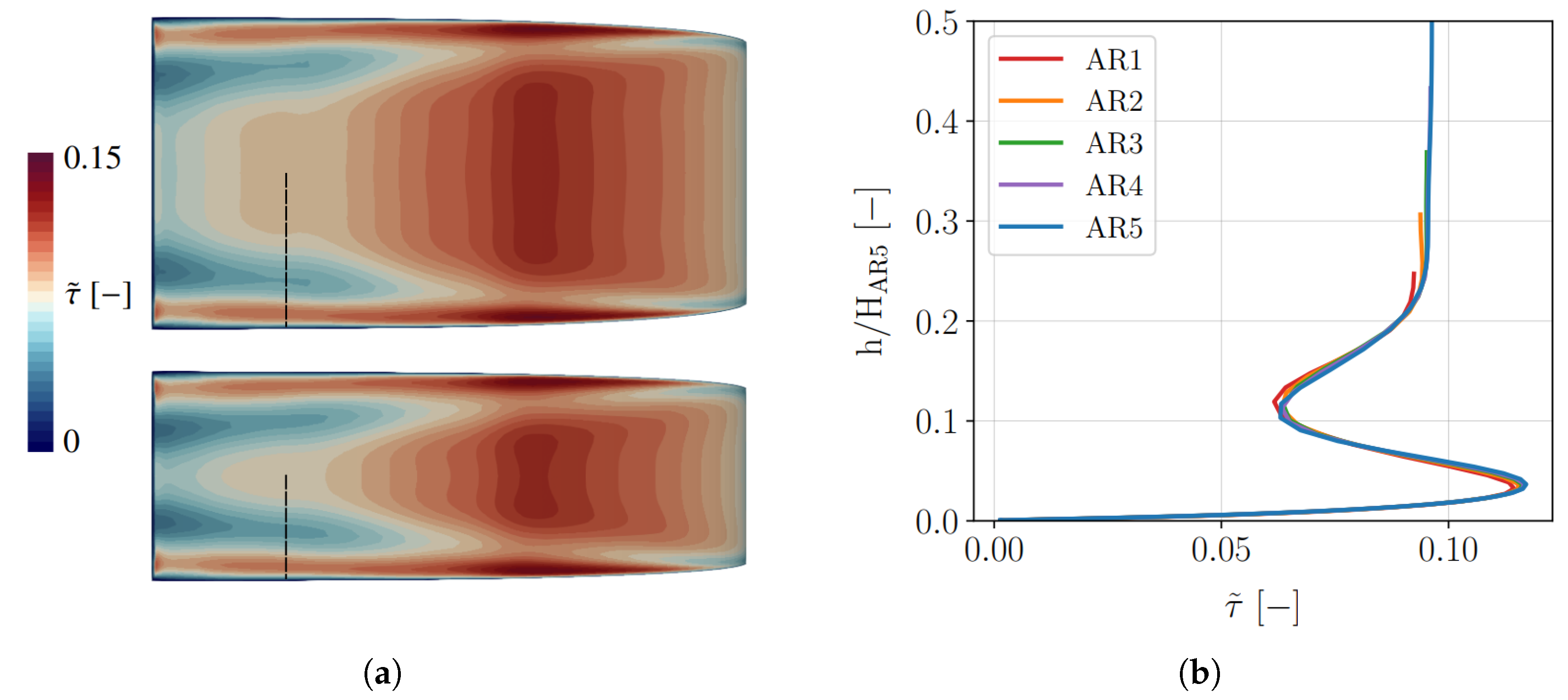
This study evaluates whether this approach of summing separate loss contributions is acceptable and quantifies its deviations from actual measured losses. For this purpose, several linear cascades and NGV simulations were run at different working points and with different features. For the linear cascade, five cases at different operating points and five cases with different aspect ratio (AR) values (obtained by modifying the span height) were created, as summarized in

Table 2. List of linear cascade cases.

Case	$\widetilde{\dot{\mathbf{m}}}$	MTE	AR	Re
Cascade M1	0.927	0.683	1	$8.4·{10}^5$
Cascade M2	0.956	0.735	1	$8.7·{10}^5$
Cascade M3	0.983	0.808	1	$8.9·{10}^5$
Cascade M4	1	0.898	1	$9.1·{10}^5$
Cascade M5	1.012	1.24	1	$9.5·{10}^5$
Cascade AR1	0.492	0.898	$0.500$	$9.1·{10}^5$
Cascade AR2	0.611	0.898	$0.625$	$9.1·{10}^5$
Cascade AR3	0.736	0.898	$0.750$	$9.1·{10}^5$
Cascade AR4	0.865	0.898	$0.875$	$9.1·{10}^5$
Cascade AR5	1	0.898	1	$9.1·{10}^5$

. Cascade M4 and Cascade AR5 refer to the same simulation, labeled differently for clarity. They are equivalent to the reference case, which corresponds to the FACTOR test rig conditions ($P_{t_0}/P_{s_1}=1.79$) and has an AR of 1. The Reynolds number is specified in the table for each case, and it was calculated at the trailing edge using the blade chord as characteristic length.

For the turbine NGV, five simulations were run at different operating points, as indicated in

Table 3. List of NGV cases.

Case	$\widetilde{\dot{\mathbf{m}}}$	MTE	AR	Re
NGV M1	0.948	0.707	1	8.7 $·{10}^5$
NGV M2	0.983	0.774	1	9.0 $·{10}^5$
NGV M3	1	0.851	1	9.2 $·{10}^5$
NGV M4	1.008	0.900	1	9.3 $·{10}^5$
NGV M5	1.012	0.961	1	9.4 $·{10}^5$

. Case NGV M3 also has the FACTOR test rig conditions. Uniform total pressure and temperature inlet boundary conditions were applied to both the cascade and NGV simulations.

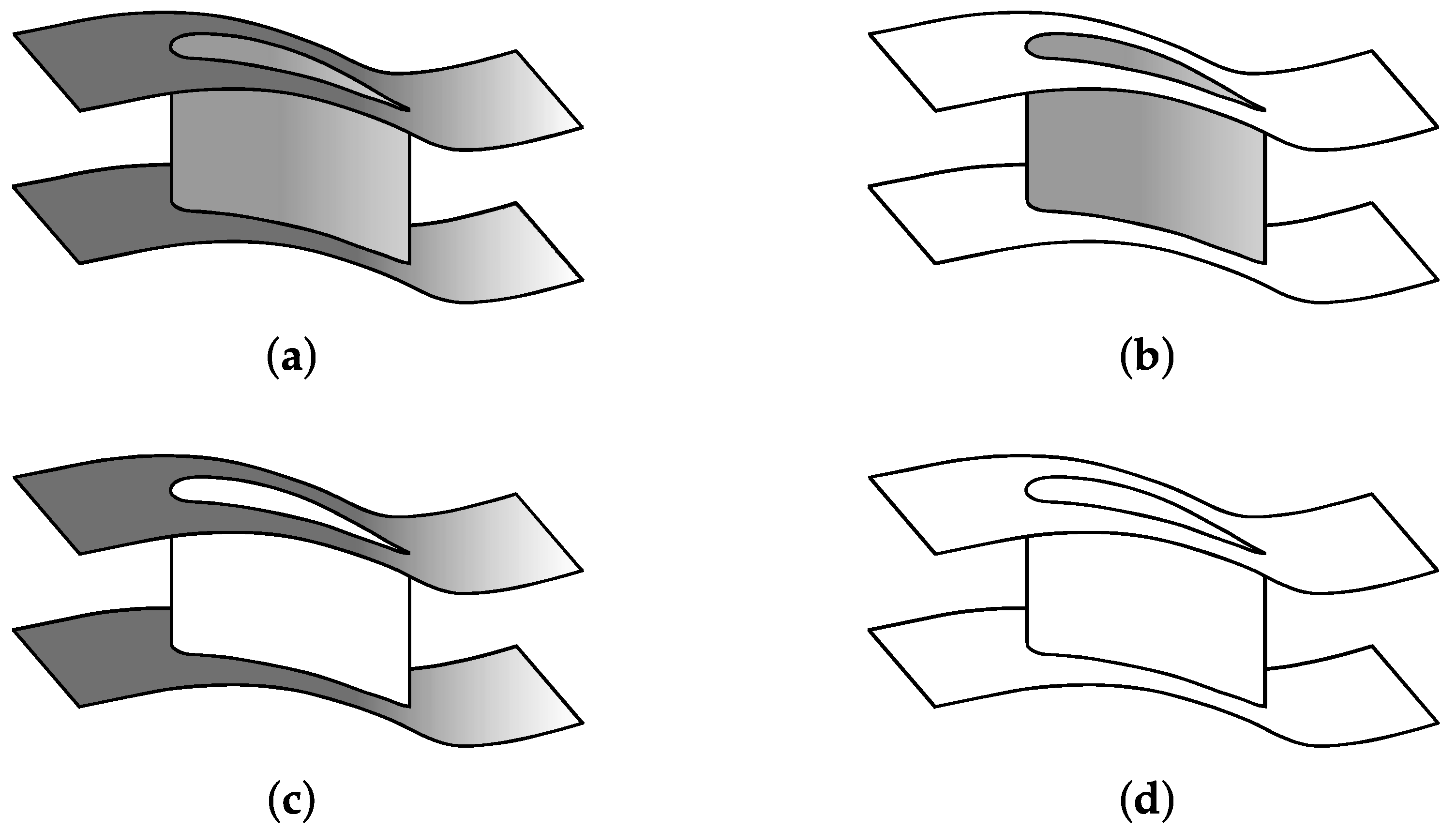
The sensitivity of nonlinearity to the mass flow and to the AR was investigated: for each of the cases in Table 2 and Table 3, multiple simulations were run with different boundary conditions. The blade surface and the endwalls were set either as no-slip walls or as slip walls. This gave rise to four different combinations, which are summarized in

Table 4. List of simulations for each Cascade and NGV case.

Case	Blade BC	End Walls BC
BC1	no-slip	no-slip
BC2	no-slip	slip
BC3	slip	no-slip
BC4	slip	slip

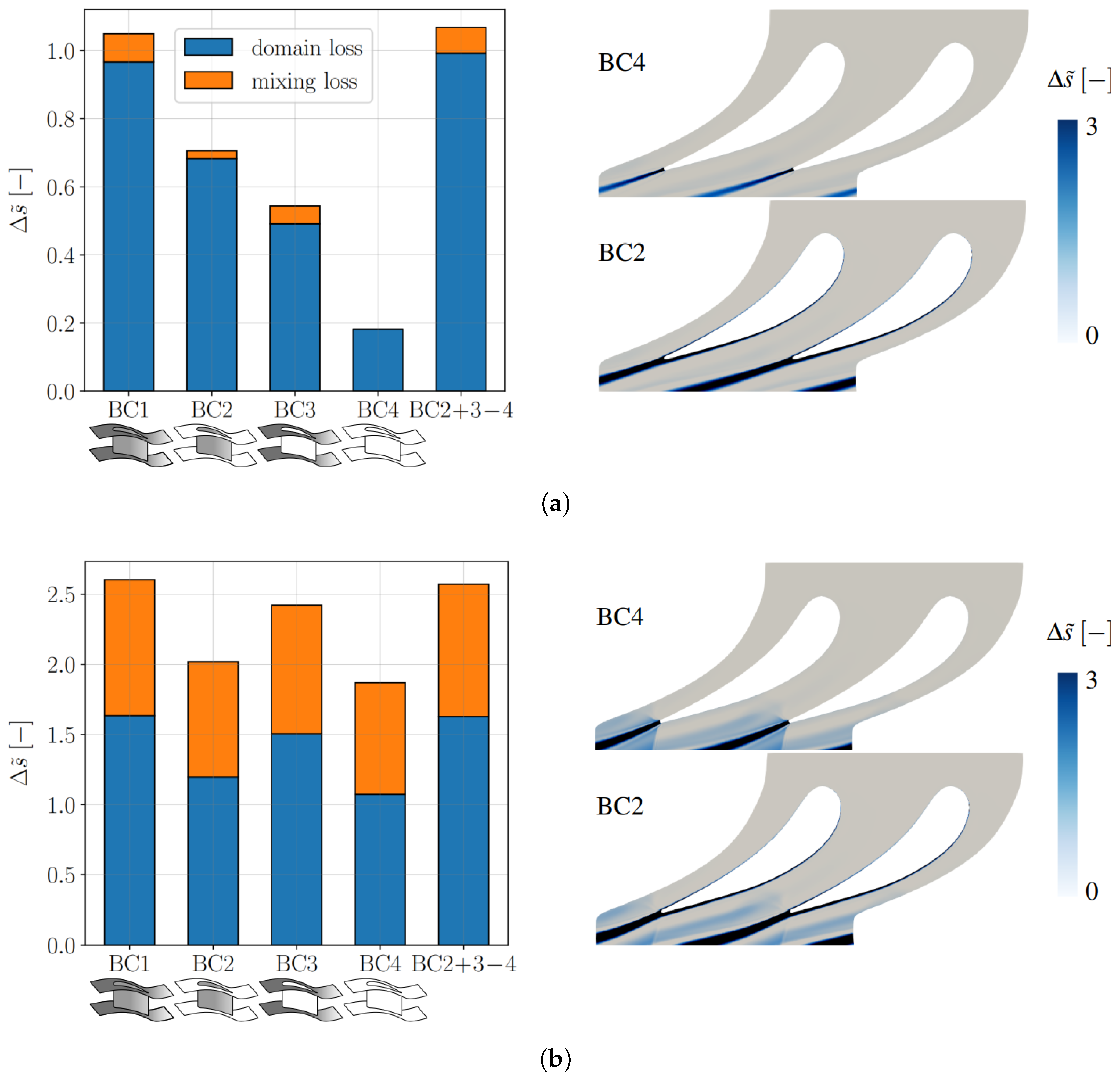
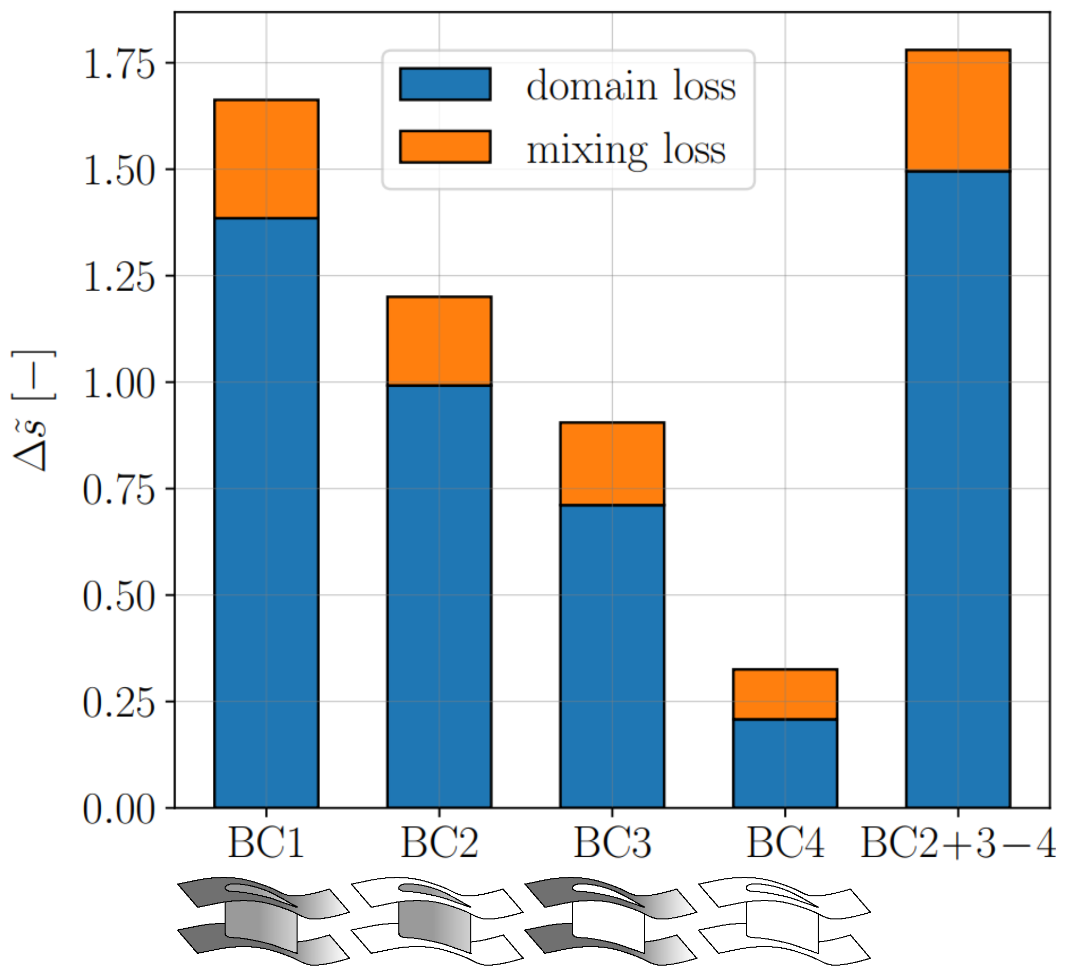
and represented in Figure 4, where no-slip walls are colored in grey and slip walls in white. Case BC1 is the realistic case, presenting boundary layers on every wall. In cases BC2 and BC3, respectively, only profile losses and endwall losses occur, together with the streamwise shear losses caused by flow turning and section variations. Finally, case BC4 only presents such streamwise shear losses.

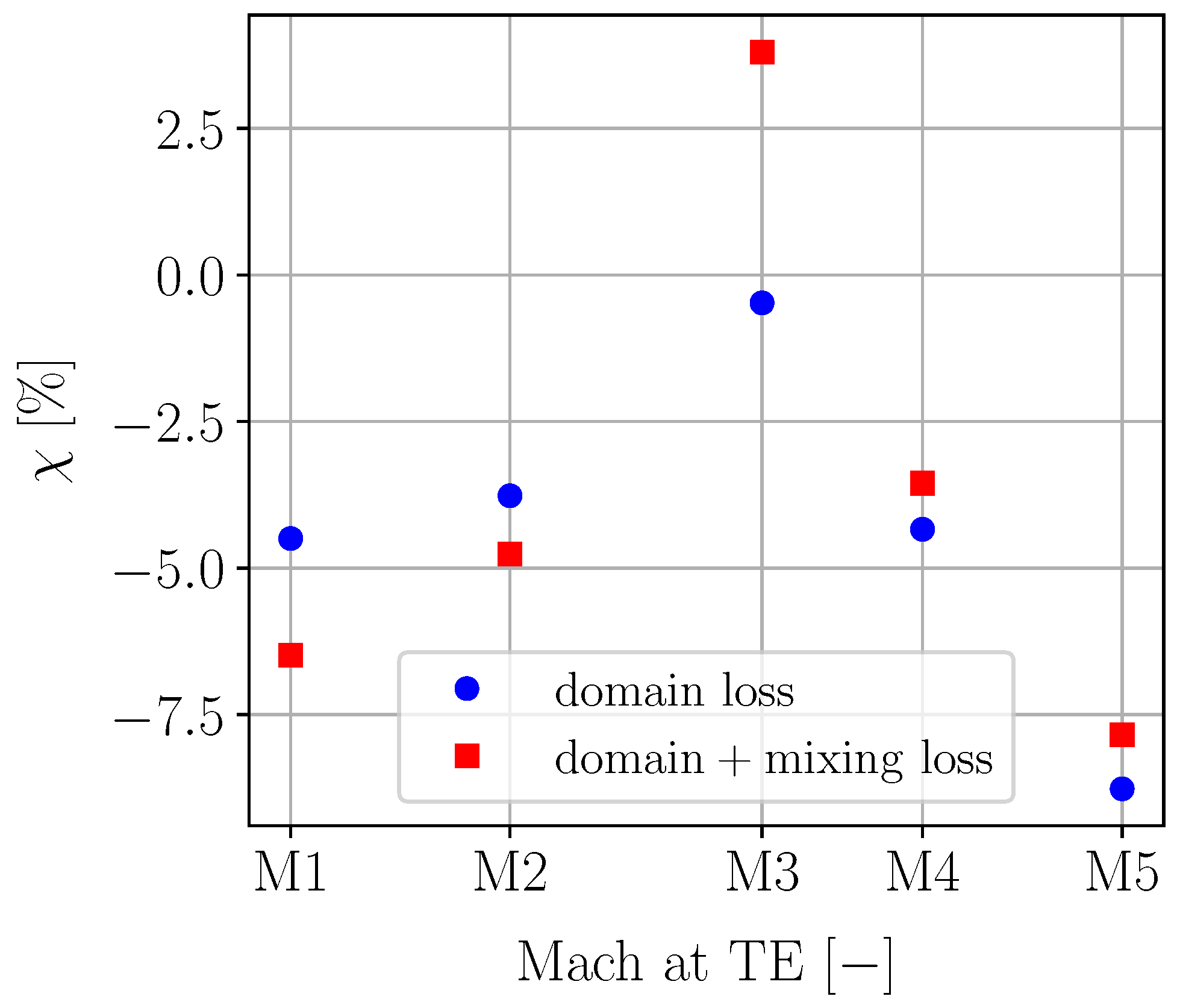
For each Cascade and NGV case, the outlet pressure was tuned to ensure that all four BC combinations reached the same mass-averaged Mach number at the trailing edge. This standardization allowed for a consistent comparison across the cases, as imposing different wall boundary conditions could otherwise lead to different operating points. Comparison at constant TE Mach number is one among various possible approaches. For instance, Yoon et al. [27] compared steady simulations with different boundary conditions while keeping the same stage pressure ratio and reaction degree. Here, the authors chose to vary the outlet pressure to maintain a constant TE Mach number to minimize variations in the operating point across different simulations. This is believed to be especially important when comparing transonic simulations, in which a slight difference in flow speed near the shock wave leads to considerable differences in the shock wave losses.

In correlations, total losses are calculated by summing the profile losses and the endwall losses. This approach is comparable to summing the losses from cases BC2 and BC3. However, shear losses occur even in the absence of boundary layers. Thus, to avoid double-counting when summing profile and endwall losses, the loss from case BC4 should be subtracted. Thus, the following question allows us to quantify the impact of nonlinearity and evaluate the validity of the summing approach for correlations:

$$\mathrm{loss}\left(\mathrm{B}\mathrm{C}1\right)⋚\mathrm{loss}(\mathrm{B}\mathrm{C}2+\mathrm{B}\mathrm{C}3-\mathrm{B}\mathrm{C}4)$$

(3)

If the loss in case BC1 is similar to that in cases BC2, 3, and 4 combined, this would support the hypothesis that loss linearity is a reasonable assumption for correlations. Conversely, if the losses differ significantly, it would suggest the presence of strong interactions among the loss sources, indicating that the assumption of loss linearity may be too restrictive. These interactions may either amplify overall losses (indicated by a positive sign in Equation (3)) or reduce them (negative sign in Equation (3)).

3. Loss Formulation

In the present work, both domain losses and downstream mixing losses are taken into account. Domain losses represent the amount of loss that occurs between the inlet and the outlet plane. If the flow has not yet reached a uniform state at the domain outlet, additional losses will necessarily occur further downstream, known as mixing losses. Evaluating mixing losses is important because the state of the flow leaving one row directly affects the loss encountered in the subsequent row. Indeed, flow inhomogeneities, such as those induced by TE wakes, can be dramatically altered by changes in free-stream velocity, as first studied by Hill et al. [28] and Smith [29]. Denton [14] demonstrated that adverse pressure gradients result in an increase in wake losses, while favorable pressure gradients attenuate wake losses (a mechanism called “wake recovery” by Smith [29]). Praisner et al. [30] later found that the former effect is significantly more pronounced than the latter for rotating blades. In contrast, Rose and Harvey [31] observed a slight reduction even in the case of diffusion. Although most authors have focused on wake losses, these mechanisms concern every kind of flow structure presenting velocity or temperature gradients. For the sake of simplicity, here, mixing losses are computed under the hypothesis that the flow mixes out to the uniform condition at a constant flow area. However, it is important to remember that, in reality, these losses still have to occur, and the downstream component will interfere with the process. Thus, this value represents potential losses, and it may vary based on the downstream conditions.

In this work, losses are expressed in terms of specific entropy $\Delta s$:

$$\Delta s=c_p\ln \left({\displaystyle \frac{T_t}{{T_t}_{in}}}\right)-r\ln \left({\displaystyle \frac{P_t}{{P_t}_{in}}}\right).$$

(4)

The difference between the mass-averaged entropy at the outlet and inlet planes (Equation (5)) gives a measure of the loss generated within the domain:

$$\Delta s=\Delta s^1-\Delta s^0.$$

(5)

To quantify the downstream mixing loss, the mixing loss potential introduced by Firrito [32] is employed. Firrito expressed loss in terms of total pressure coefficient:

$$Y^{mix}={\displaystyle \frac{{{P_t}_1}^m-{{P_t}_1}^{MO}}{{{P_t}_1}^{MO}}},$$

(6)

where m stands for mass average and $MO$ stands for mixed-out average. The mixed-out average formulation used in this work is the one introduced by Prasad [33] in the Cartesian coordinate system for the curved duct and linear cascade configurations and in the cylindrical coordinate system for the NGV. Prasad derived the mixed-out state from the initial nonuniform state (here, the outlet plane 1) by enforcing the conservation of mass, momentum, and energy between the two states. Here, an equivalent entropy expression is derived under the hypothesis of constant total temperature:

$$\Delta s^{mix}=-r\ln \left({\displaystyle \frac{{{P_t}_1}^{MO}}{{{P_t}_1}^m}}\right)$$

(7)

The total losses, including domain and mixing losses, can therefore be expressed as:

$$\Delta s+\Delta s^{mix}=-r\ln \left({\displaystyle \frac{{{P_t}_1}^m}{{{P_t}_0}^m}}\right)-r\ln \left({\displaystyle \frac{{{P_t}_1}^{MO}}{{{P_t}_1}^m}}\right)$$

(8)

To evaluate the losses resulting from interactions between various phenomena, 3D losses were estimated alongside the entropy balance discussed above. For this purpose, a loss audit was performed with a tool developed by the authors, which is described in [22]. This tool allows the identification of several loss-generating mechanisms from 3D RANS solutions (boundary layers, vortices, shock waves, TE wakes, and streamwise shear) by using detection criteria based on flow quantities. The losses related to each phenomenon are quantified in terms of the viscous entropy generation rate, which is computed in the whole 3D domain. In [22], a priority order was established for allocating losses among various sources; for instance, in the case of domain cells meeting the detection criteria of both the shock wave and the boundary layer, such cells were allocated to the latter. This approach ensured that losses were not attributed to multiple mechanisms simultaneously. In the present study, a new feature has been introduced to the tool: the ability to quantify losses arising from interactions. This is achieved by identifying all domain cells that meet multiple detection criteria concurrently. As a result, interactions can be treated as distinct phenomena, contributing separately to the overall flow losses.

4. Results

4.1. Curved Duct: Boundary Layer–Vortex Interaction

Domain losses and mixing losses of the curved duct simulations introduced in Table 1 were computed and compared, to better understand the role of interactions between the boundary layers and the injected vortex.

4.1.1. Quantitative Analysis

Figure 5 shows the domain and mixing losses generated in all the Duct cases. It can be seen that the overall losses are consistently lower when the vortex is injected closer to the wall compared with when it is positioned at the center of the inlet (meaning that the losses from Duct3 are lower than those from Duct2, the losses from Duct6 are lower than those from Duct5, and the losses from Duct9 are lower than those from Duct8).

This trend also holds when examining mixing losses alone, which seems reasonable since the central vortex drags a bigger portion of the surrounding flow and creates a less homogeneous flow compared with the corner vortex. This also applies when considering domain losses alone, but only in the presence of boundary layers (with only slight differences between Duct5 and Duct6). Indeed, in the absence of boundary layers, the opposite effect is observed. This suggests that the interaction between the corner vortex and the boundary layers, which is believed to be more intense than that between the center vortex and the boundary layers, contributes to reducing the overall losses (or mitigating their increase).

Corner and passage vortices, which form due to boundary layers and pressure gradients in the curved part of the duct, are also involved in the flow dynamics. Such vortices are already present in Duct4 (Figure 6a), but their shape and trajectory can be modified when a vortex is injected at the inlet and interaction occurs. Figure 6b shows that, in Duct6, the upper corner and passage vortices are not influenced by the presence of the injected vortex. However, the lower vortices change substantially compared with those in Duct4: in the right corner, which is close to the injected vortex, a smaller counter-rotating vortex is generated not far from the inlet. The left corner vortex develops a second branch, which originates from the boundary layer and the motion induced by the injected vortex. Towards the end of the curve, the left passage vortex cannot merge with the right corner vortex, as they are kept separated by the injected vortex. Case Duct5 is not shown here; however, it was observed that, once again, the upper vortices are very similar to those in Duct4. One might expect that the central injected vortex, being introduced at mid-span, would affect both the upper and the lower passage vortices. However, its clockwise rotation causes it to move closer to the lower wall in the curved section (this is visible in Figure 7). Thus, it mostly influences the lower passage vortex, which remains similar in shape to that of Duct4 but thicker in comparison.

The loss trend of cases from Duct4 to Duct6 confirms that of [22], in which the same three simulations were studied and losses were estimated in terms of entropy generation rate computed on the whole 3D volume. Similar comments can be made about cases from Duct7 to Duct9. More nonlinearity is observed compared with the slower cases, suggesting that the average flow speed might have an impact on the boundary layer–vortex interactions. The significantly high mixing losses in the last three cases, as well as their higher nonlinearity, are attributed to the presence of a shock wave that was observed at the duct throat, resulting in highly nonuniform flow at the outlet plane.

As mentioned in Section 2.1, comparison between cases from Duct1 to Duct6 allows us to roughly quantify the interaction between the two main loss sources present in the duct: the boundary layer and the vortex. The center and corner vortex losses can be estimated by subtracting the Duct1 losses (which primarily arise from streamwise shear due to the duct shape) from the Duct2 and Duct3 losses, respectively. Similarly, boundary layer losses—including the related corner and passage vortices of Figure 6a—can be determined by subtracting the Duct1 losses from the losses observed in Duct4. Afterward, the sum of these separate losses can be compared with the actual loss measured in cases Duct5 and Duct6: the difference represents the impact of interactions. In Figure 5, the losses obtained by summing the separate contributions are indicated with a dashed line superposed to the actual loss of Duct5 and Duct6. This suggests that the hatch-patterned region consists of domain and total losses resulting from the boundary layer–vortex interaction, including the subsequent changes in the formation of passage vortices. It can be concluded that the impact of interactions is weak in Duct6, while it is more detrimental in Duct5. A similar study was conducted comparing cases Duct8 and Duct9 with their equivalent slip-wall cases (not presented in this paper) and yielded similar results. Overall, losses due to interactions were higher than those observed in Duct5 and Duct6, likely due to the greater average flow speed. However, the same trend persisted, with the central injected vortex case exhibiting higher nonlinearity than the corner injected vortex case in both the domain and total losses. To ensure that the results were not influenced by the selection of a specific outlet plane location, the study was repeated with the curved duct outlet plane shifted from $\tilde{\mathrm{x}}=1$ to $\tilde{\mathrm{x}}=1.5$. The same trend was observed, with an even more pronounced difference in overall losses between the center and corner vortex cases.

4.1.2. Qualitative Analysis

Figure 7 helps us understand the differences between the cases with central vortex and those with corner vortex in terms of BL–vortex interactions.

It shows the entropy distribution on a vertical plane that passes along the vortex trajectory in the curved part of the duct. Cases Duct2 and Duct3 are represented in the upper part of the figure: it can be seen that the high entropy area, which corresponds to the presence of the vortex, is approximately the same size for both the center and the corner vortex. In the bottom part of the figure are cases Duct5 and Duct6, which present a boundary layer. In case Duct6, the proximity of the corner vortex to the bottom wall boundary layer causes an interaction between the two phenomena, which seems to limit the boundary layer extension and mitigate losses. This interaction and proximity to the wall also cause the corner vortex to drag a smaller portion of the surrounding free-stream flow, thus dissipating faster. This results in lower mixing losses downstream of the outlet plane with respect to case Duct5. These results are in good agreement with the findings of Montsarrat [34], who studied the evolution with time of two counter-rotating vortices. Montsarrat observed that, as the vortices merge to form a dipole, their interaction leads to a reduction in circulation magnitude, leaving behind vorticity trails. The same phenomenon can be observed here between the vortex and the boundary layer. It is now clear why case Duct6 presents less nonlinearity than case Duct5 in Figure 5: stronger interactions occur between the corner vortex and the bottom boundary layer, but such interactions simultaneously help to contain both phenomena. Conversely, the center vortex has weaker interactions with the boundary layer, but these losses accumulate with those already generated by the two separate phenomena. While the entropy field seems to reach higher values in the right images compared with the left ones, this discrepancy is primarily due to the fact that the center and corner vortices follow slightly different trajectories in the curved part of the duct. The upper left schematic in Figure 7 illustrates these trajectories, justifying the selection of the cut plane and indicating the viewing direction.

4.2. Linear Cascade: Nonlinearity Assessment

As for the curved duct, domain losses and mixing losses were calculated for all the linear cascade cases (Table 2) and all their BC combinations (Table 4). The following paragraphs analyze the sensitivity of nonlinearity to variations in the operating point and in the aspect ratio. To serve this purpose, a nonlinearity coefficient $\chi$ is introduced, which measures the difference in losses between the case presenting all loss sources simultaneously (BC1) and the combination of the single-source cases (BC2 + BC3 − BC4). It is expressed as

$$\chi [\%]={\displaystyle \frac{\Delta s^{\left(\mathrm{B}\mathrm{C}1\right)}-\Delta s^{(\mathrm{B}\mathrm{C}2+\mathrm{B}\mathrm{C}3-\mathrm{B}\mathrm{C}4)}}{\Delta s^{\left(\mathrm{B}\mathrm{C}1\right)}}}·100.$$

(9)

When $\chi$ is close to zero, the nonlinearity effect is negligible. A positive value indicates that the interaction between different wall boundary layers increases overall losses. Conversely, a negative value suggests that these interactions reduce total losses, providing a beneficial effect.

4.2.1. Sensitivity to the Mach Number

The bar chart in Figure 8a shows the losses generated by the different BC cases of Cascade M4. It can be seen that while the domain losses generated by the blade BL (BC2) are higher than those of the endwall BL (BC3), the mixing losses are higher in case BC3 than in case BC2. This is consistent with what was expected: indeed, the TE wake is already partially mixed out at the outlet plane, while the endwall BL represents a strong nonuniformity and occupies a larger portion of the outlet plane (since the pitch is equal to the span). The right bar (BC2 + BC3 − BC4) indicates that when profile and endwall losses are assessed individually and then combined, the total loss is only marginally higher than the actual measured loss (case BC1). On the right side of the figure is the mid-span entropy field for cases BC4 (above) and BC2 (below). The trailing edge wake varies considerably depending on whether the blade boundary layer is absent or present; indeed, in the former case (BC4), the wake results exclusively from the velocity difference between the suction and pressure sides. Its intensity aligns with the corresponding mixing loss results. Bar charts for Cascades M1 to M3 are omitted due to space constraints, but they show the same trend for cases BC1 to BC4 in terms of domain and mixing losses.

The same bar chart is proposed for Cascade M5, which has a supersonic TE Mach number, in Figure 8b. It can be observed that the overall losses are around $2.5$ times higher than in Cascade M4 despite the very little rise in mass flow rate, suggesting that the shock wave is responsible for most of the additional loss. Moreover, the trend is very different from the subsonic cases: mixing losses experience a significant increase, even in the absence of boundary layers (BC4), confirming the significant role of shock waves in loss generation. The explanation can be found in the entropy field on the right side of the figure: in case BC4, the TE wake, which was relatively weak in Cascade M4, is now nearly as strong as in case BC2. This change is attributed to the shock wave being located at the trailing edge, which is a typical shock configuration for 2D blades. Furthermore, the domain losses of case BC3 are now higher than those of BC2. The small difference between BC2 and BC4, as well as between BC1 and BC3, indicates that losses due to the blade boundary layer are almost negligible in this transonic configuration. This is again explained by the fact that the shock wave does not interact with the blade boundary layer (a case of interaction between the shock wave and the blade BL will be studied in Section 4.3 using the NGV configuration). All these observations indicate that, although a linear relationship appears to exist, the situation is more complex than it initially seems: the presence of a shock wave causes a considerable entropy rise in all BC cases, which tends to standardize the four cases and creates an appearance of linearity. However, the main conclusion to be drawn is that quantifying nonlinearity in the presence of a shock wave is extremely complex. This also suggests that representing shock wave losses merely as a correction factor in a profile loss correlation, as is commonly done, may be inadequate.

The nonlinearity coefficient $\chi$ (Equation (9)) for the linear cascade as a function of the Mach number is shown in Figure 9—both for domain losses and for total losses, including downstream mixing. It can be seen that the nonlinearity coefficient decreases in magnitude as the Mach number approaches the value of Cascade M4, which corresponds to the FACTOR test rig operating point. As already discussed, Cascade M5 seems very close to linearity between case BC1 and cases BC2+BC3-BC4, but the reality is more complicated than that due to the presence of the shock wave. What is less intuitive is that the nonlinearity coefficient takes on negative values. This means that the realistic case (BC1) generates fewer losses than the combination of cases BC2 to BC4 for all Cascade M* simulations.

4.2.2. Sensitivity to the Aspect Ratio

Figure 10 shows the nonlinearity coefficient as a function of the AR. As expected, Cascade AR5, which has the largest AR, has the highest linearity. Indeed, it can be anticipated that stronger interactions will occur as the upper and lower vortices come closer together. An almost linear relationship between AR and $\chi$ is observed. As in Figure 9, $\chi$ takes negative values. This may be explained by the overlap between the blade and end wall BL at the corners, which remains constant in size as the blade span decreases, leading to a proportionally greater impact on overall losses.

Figure 11a shows the distribution of the normalized skin friction coefficient along the suction side of the blade for Cascades AR3 and AR1. It can be seen that in Cascade AR3, the upper and lower secondary flows are quite distinct, while in Cascade AR1, they have partially merged. This aligns well with the proportionality observed in Figure 10. However, the distribution of $\tilde{\tau }$ near both the hub and shroud appears to remain unchanged, regardless of the aspect ratio. This is even more evident in Figure 11b, which presents the spanwise evolution of $\tilde{\tau }$ along the half-span for all Cascade AR*, with the profiles of the different cases perfectly aligned. This suggests that a characteristic size of the secondary flow losses, based on blade parameters other than the aspect ratio, could be identified. This would provide insight into when interactions between the upper and lower structures might begin to occur.

As explained in Section 3, a loss audit tool developed by the authors was also employed to quantify the amount of interactions taking place in cases Cascade AR1 to AR5.

Table 5. Losses due to interactions between boundary layers (BL), vortices (V), and wakes (W) in Cascade AR* cases.

Cascade	BL-V [%]	V-W [%]	BL-W [%]	Tot [%]
AR1	1.77	0.40	0.13	2.31
AR2	1.59	0.36	0.13	2.08
AR3	1.45	0.30	0.12	1.87
AR4	1.33	0.28	0.11	1.72
AR5	1.24	0.24	0.10	1.58

shows the amount of loss due to interactions expressed as a percentage of the total volume losses. Various types of interactions are assessed—considering boundary layers, vortices, and TE wakes—with the interaction between boundary layers and vortices accounting for the largest portion of the total. Looking at the five cascade cases, it can be observed that the contribution of interactions decreases as the AR value increases. The trend concerns both the total values and each of the separate types of interaction, further confirming the decrease in interactions for increasing AR values observed in Figure 11a.

4.3. Turbine NGV: Nonlinearity Assessment

The sensitivity of loss linearity to the operating point was analyzed on a turbine NGV configuration. The aim was to determine whether a twisted annular geometry could yield significantly different results than a linear cascade in terms of loss linearity. Figure 12 shows the nonlinearity coefficient for the five NGV simulations listed in Table 3. Compared with the linear cascade results, higher levels of nonlinearity can be observed in this 3D configuration, especially as far as the off-design simulations (NGV M1, M2, M4, and M5) are concerned.

Case NGV M5 is a realistic example of a slightly transonic high-pressure turbine vane. The losses generated by the different BC cases for NGV M5 are shown in Figure 13. Contrarily to the case of Cascade M5 (Figure 8b), the increase in domain and mixing losses here is less substantial (around $25\%$ increase with respect to NGV M3 losses). The reason is that the shock wave is weaker in the NGV configuration, and it is located well before the TE, as is usually the case in transonic high-pressure turbines. It was observed that fewer losses occured when the shock wave interacted with the blade boundary layer (NGV M5) compared with when the interaction occurred at the trailing edge (Cascade M5). Despite this and the reduced intensity of the shock wave, nonlinearity effects are higher in the NGV configuration, indicating that the complexity of the domain contributes to the extent of these effects.

5. Conclusions and Future Perspectives

This work aimed to investigate how various loss-generating mechanisms interact with each other in axial flow turbines and the consequences of these interactions on the overall losses. Three geometries progressively resembling an industrial turbine were selected, and 3D RANS simulations were run with multiple combinations of inlet and wall boundary conditions in order to observe loss sources both individually and simultaneously. Both domain losses and mixing losses were estimated for each simulation and expressed in terms of entropy.

The curved duct geometry allowed us to analyze the boundary layer–vortex interaction for two different vortex positions. It was found that when the vortex is sufficiently close to the wall, its interaction with the boundary layer helps to contain both phenomena, resulting in minimal additional losses and faster vortex dissipation. In contrast, when the vortex is positioned farther from the walls, a great portion of the free stream is involved in its interaction with the boundary layers, causing significant losses. This behavior becomes more pronounced for higher mass flow rates. The linear cascade and turbine NGV geometries enabled us to further investigate the role of loss interactions, helping to determine whether the hypothesis of loss linearity is an acceptable approach in correlations. It was observed that the operating point, the aspect ratio, and the complexity of the geometry under consideration can all influence the linearity of losses. While linearity does not seem too far from reality in the linear cascade study, results for the turbine NGV show higher nonlinearity and less predictable patterns.

Future perspectives of this work include investigating the effects of interactions and assessing the validity of the loss linearity hypothesis in rotating blade geometries. Indeed, interactions are generally more pronounced in rotor blades than in vanes, with a less homogeneous flow at the blade inlet, potentially further compromising linearity.

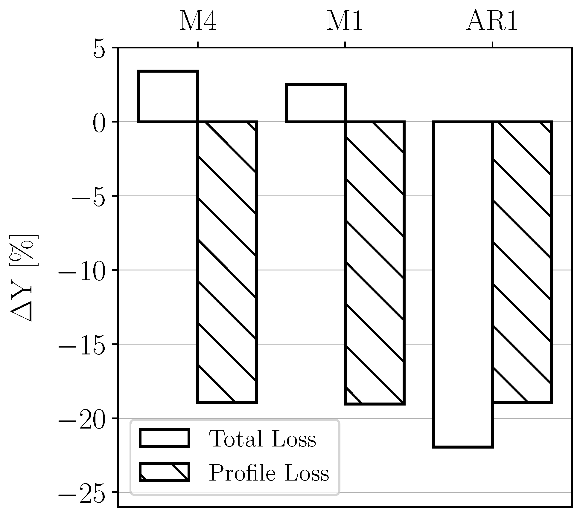
This work constitutes a modest yet meaningful contribution toward the broader objective of improving loss prediction in the pre-design phase. As an example, Figure 14 shows the relative difference between losses predicted via the well-known Ainley and Mathieson (AM) correlation [2] and losses derived from the CFD simulations presented in this work. The total losses obtained through the 3D simulations show good agreement with those predicted by the 0D model for Cascades M4 and M1. However, this is not the case for Cascade AR1, as the AM correlation does not account for the aspect ratio. Additionally, the profile losses are underestimated by the AM model when compared with losses of cases BC2, likely due to the blade’s considerably greater thickness—almost double the maximum value within the range used to establish the profile loss correlation. Finally, it is worth noticing that since the AM correlation is based on metal and flow angles calculated at mid-span, it struggles to distinguish between the losses of the NGV configuration and those of the linear cascade (obtained by extruding the NGV mid-span profile), particularly when the mid-span flow angles are similar.

Considering the role of nonlinearity, as investigated in this paper, the next step will involve examining the sensitivity of various loss sources to different flow and geometric parameters in order to improve and expand the validity range of existing correlations.