Article

Computational Design of an Energy-Efficient Small Axial-Flow Fan Using Staggered Blades with Winglets

1
Department of Energy Systems Engineering, Engineering Faculty, 50th Campus, Ankara University, Bahcelievler, Ankara 06830, Turkey
2
Department of Mechanical Engineering, Engineering Faculty, Yasar University, Izmir 35100, Turkey
*
Author to whom correspondence should be addressed.
Int. J. Turbomach. Propuls. Power 2025, 10(1), 1; https://doi.org/10.3390/ijtpp10010001
Submission received: 5 April 2024 / Revised: 20 November 2024 / Accepted: 29 November 2024 / Published: 9 January 2025

Abstract

:
The present study introduces a conceptual design of a small axial-flow fan. Both individual and combined effects of blade stagger angle and winglet on the performance of the fan design are investigated in design and off-design operating conditions using a computational flow methodology. A stepwise solution, in which a proper stagger angle adjustment of a specifically generated blade profile is followed by appending a winglet at the tip of the blade with consideration of different geometrical parameters, is proposed to improve the performance characteristics of the fan. The initial model comparison analysis demonstrates that a three-dimensional, Reynolds-averaged Navier–Stokes (RANS) equation-based renormalization group (RNG) kε turbulence modeling approach coupled with the multiple reference frame (MRF) technique which adapts multi-block topology generation meshing method successfully resolves the rotating flow around the fan. The results suggest that the use of a proper stagger angle with the winglet considerably increases the fan performance and the fan attains the best total efficiency with an additional stagger angle of +10° and a winglet, which has a curvature radius of 6.77 mm and a twist angle of −7° for the investigated dimensioning range. The present study also underlines the effectiveness of passive flow control mechanisms of the stagger angle and winglets for energy-efficient axial-flow fans.

1. Introduction

An axial-flow fan is the most common type of fan which moves an air or gas stream along the axis of rotation while a centrifugal or radial flow fan moves an air or gas stream perpendicular to the axis of rotation. Axial-flow fans, which are better suited to low-resistance, high-flow applications, are used for cooling of electronic devices due to their low-pressure resistance, low weight, and simple construction [1]. In small-scale applications, generally an axial-flow fan is preferred due to the fact that a centrifugal fan has a more complicated structural design than an axial fan. Nowadays, small axial-flow fans are prevalently used in many different applications such as air heat exchangers for chemical processes, cooling for various types of electrical devices, motors, and generators, and humidifiers in textile mills [2].
Although small axial-flow fans are generally considered to have the ability to generate greater air movement with considerably less energy consumption, aerodynamic performance and energy efficiency analysis of such fans has been investigated both experimentally and numerically [3,4,5,6,7,8,9,10,11,12,13,14,15,16,17,18,19,20,21,22,23,24] over the last two decades through aerodynamically effective fan design parameters such as total head, volumetric flow rate, rotor diameter, leakage flow, and blade profile to further improve aerodynamic and/or aeroacoustic performance. In consideration of aerodynamic performance enhancement of small-scale axial fans with special emphasis on design optimization of fan blades, there are a great number of experimental and/or numerical studies in the literature. The fan blade is considered to have the principal contact surface with the airflow for energy transfer and possess the potential to be improved [4].
Dwivedi and Dandotiya [2] conduct a numerical study including a comparative analysis between forward and backward skewed blades at two different rotational speeds. Sahu and Bartaria [6] provide an inverse design approach to determine optimum shapes for the fan blades. The effect of blade angle of attack on the fan performance is further investigated [7,8,9] through velocity and pressure field predictions between the inlet and outlet of the fan. Hirano et al. [10] perform a more specific blade optimization study in which the relationship between design parameters such as blade chord length, camber and blade setting angle, and performance characteristics is examined by a multi-regression analysis using computational data. There are also shape optimization studies including analysis of the effect of blade tip grooving [12] and that of hollow blade root [13] in the literature. Zhang et al. [13] achieve a parametric modeling and stagger angle optimization to improve fan performance. In their study, stagger angles of blade tip clearances are optimized to reduce the influence of inlet shock loss as well as a leak in blade tip clearance and hub resistance at the blade root. The effect of blade numbers is extensively studied by Zhang and Jin [14]. Mao et al. [15] propose the use of a tip end-plate to improve the noise performance of small axial fans. They adopt both numerical simulations and experimental methods to study the fluid flow and noise level of axial fans. Yang et al. [16] design inlet guide vanes with different outlet angles which are mounted on the casing and located at the upstream of the impeller of the prototype fan. Effects of the inlet guide vanes on the static characteristics, aerodynamic noise, and internal flow characteristics of the fan are studied. Yadegari et al. [20] numerically investigate the effect of utilizing a perforated surface as an innovative flow control method to reduce fan noise.
The above-summarized investigations mainly suggest passive flow control techniques be implemented on optimizing three-dimensional (3-D) shape and/or configuration of axial-flow fan blades for desired airflow rate, noise reduction, and/or pressure increase through computational fluid dynamics (CFD)-based flow analysis of the fan. Computational fluid dynamics (CFD) methodology is a very powerful design and analysis tool in turbomachinery [25] as it provides a time- and cost-effective solution to highly 3-D, turbulent, and transient flow phenomena in rotating turbomachines such as compressors and fans. The study of the passive control techniques for fans mainly originates from the aerodynamics of the blades whose performance can be improved with suppression of the flow separation [26].
In the present study, the blade profile of a small axial-flow fan is computationally generated through a stepwise solution in which a proper stagger angle adjustment is followed by appending a winglet at the tip of the blade with consideration of different geometrical parameters to improve the aerodynamic performance and hence the efficiency of the fan. With the proposition of this two-stage stepwise solution approach, not only is flow separation from the blade surface controlled through a proper stagger angle but the vorticity distribution around the tip of the blades is also controlled/minimized to some extent through the use of an appropriate winglet for higher aerodynamic performance. Winglets have been commonly used in aircraft for over a century and recently become influential devices for decreasing the tip vortices and hence improving the blade’s performance in wind turbines [27,28,29,30,31,32]. Previous numerical studies [29,30,31] demonstrate that flow patterns of aircraft winglets and horizontal axis wind turbine (HAWT) winglets differ from that of vertical axis wind turbine (VAWT) winglets so different winglet design approaches may be required depending upon the principal rotation direction of the wind turbines. Johansen and Sorensen [27] investigate the effect of several different winglet designs on the performance of wind turbines by using winglets which have height of 1.5 percent of the rotor radius and cant angle of 90° but different NACA airfoil sections and twist angles. Li [28] suggests that the main structural parameters of a winglet include inclination, lead edge sweep, height, root chord, tip chord, etc. An early study of Saravanan et al. [29] considers a winglet’s height, sweep angle, cant angle, curvature radius, toe angle, and twist angle as principal design parameters. It is reported in this study that winglet height and curvature radius are more dominant than the other parameters. The orthogonal experimental design (OED) analysis of Zhang et al. [30] further demonstrates that the twist angle is the most influential parameter so that special attention should be paid to the twist angle in the primary optimization of the winglet configuration. Cai et al. [31] state that there are two main types of winglets, up single type and up–down shifted type. Dejene et al. [32] recently computationally investigated an NREL Phase VI wind turbine blade using ten different winglets which are generated with different height, lengths, and cant angles and a simple linear tip extension. The study suggests that curving the tip to make a winglet shape of applicable configuration is preferable to extending the tip straight. Moosani et al. [17], on the other hand, improve the performance of a partially shrouded axial-flow fan by modifying the blade tip geometry and manipulating the trajectory of TLV. For this, the blade tip chord is modified to be in the axial direction before reaching the shrouded part to reduce the blockage and negative component of tip leakage flow. By cambering the blade at the tip section, the core flow also moves to lower spans which further reduces the blockage and tip loss.
A three-dimensional (3-D), Reynolds-averaged Navier–Stokes (RANS) equation-based two-equation turbulence modeling approach together with enhanced wall treatment are used here for turbulent flow-field analysis. A multiple rotating reference frame (MRF) mesh interface approach is employed to couple the rotating and stationary flow zones for flow analysis of the final rotor geometry on-design condition. The computational results are validated against the experimental data available in the open literature for the generated baseline model geometry.

2. Computational Methodology

2.1. Governing Flow Equations

For the turbulent flow of an incompressible, Newtonian viscous fluid with constant transport properties, the Reynolds-averaged Navier–Stokes (RANS) equation and continuity equation in the absence of body forces in the Cartesian tensor notation are obtained as below:
ρ D u i ¯ D t = p ¯ x i + x j μ u i ¯ x j + u j ¯ x i 2 3 δ i j u i ¯ x i + x j ρ u i u j ¯
u i ¯ x i = 0
where ρ is the fluid density, u i ¯ is the time-averaged velocity, u i is the deviation from the time-averaged velocity, p ¯ is the time-averaged pressure, μ is the dynamic viscosity of the fluid, ρ u i u j ¯ is the Reynolds stress tensor which is defined as:
ρ u i u j ¯ = 2 3 ρ k δ i j + μ t u i ¯ x j ¯ + u j ¯ x j + 2 3 μ t u j ¯ x j δ i j
where μ t is the eddy viscosity and k is the turbulent kinetic energy defined as:
k = 1 2 u i u i ¯
The Reynolds stress which appears on the right-hand side of Equation (1) actually arises from the convective terms of the Navier–Stokes equations but is treated as a diffusion term in the time-averaged Reynolds equations. Since the turbulent stresses are still unknown, it is necessary to form a closed set of equations using turbulence models to account for the effect of turbulent motion. To close the above time-averaged equations, the additional Reynolds stress term is modeled using two-equation turbulence models based on the Boussinesq hypothesis which states that the transfer of momentum generated by turbulent eddies be modeled by an eddy viscosity.

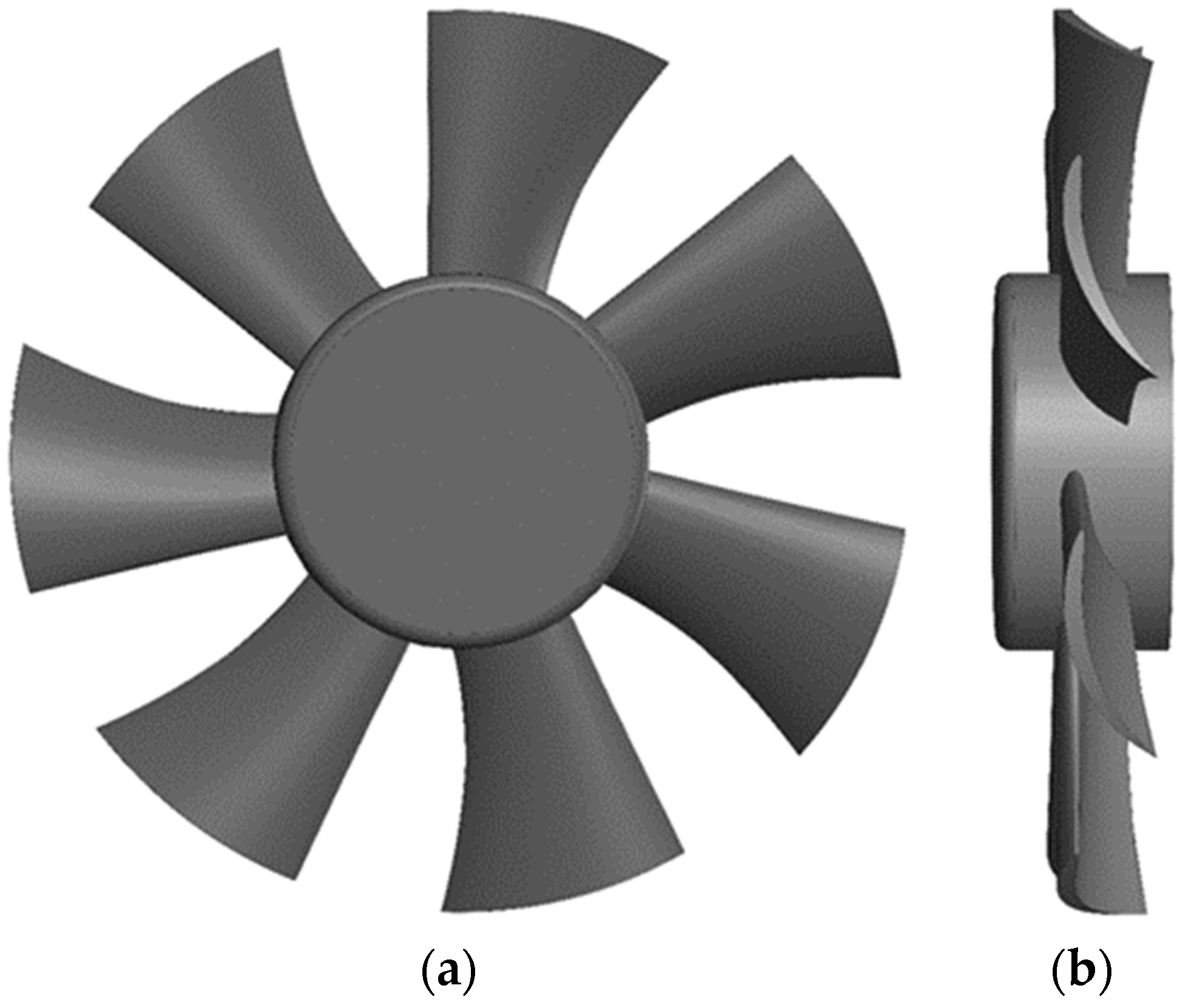
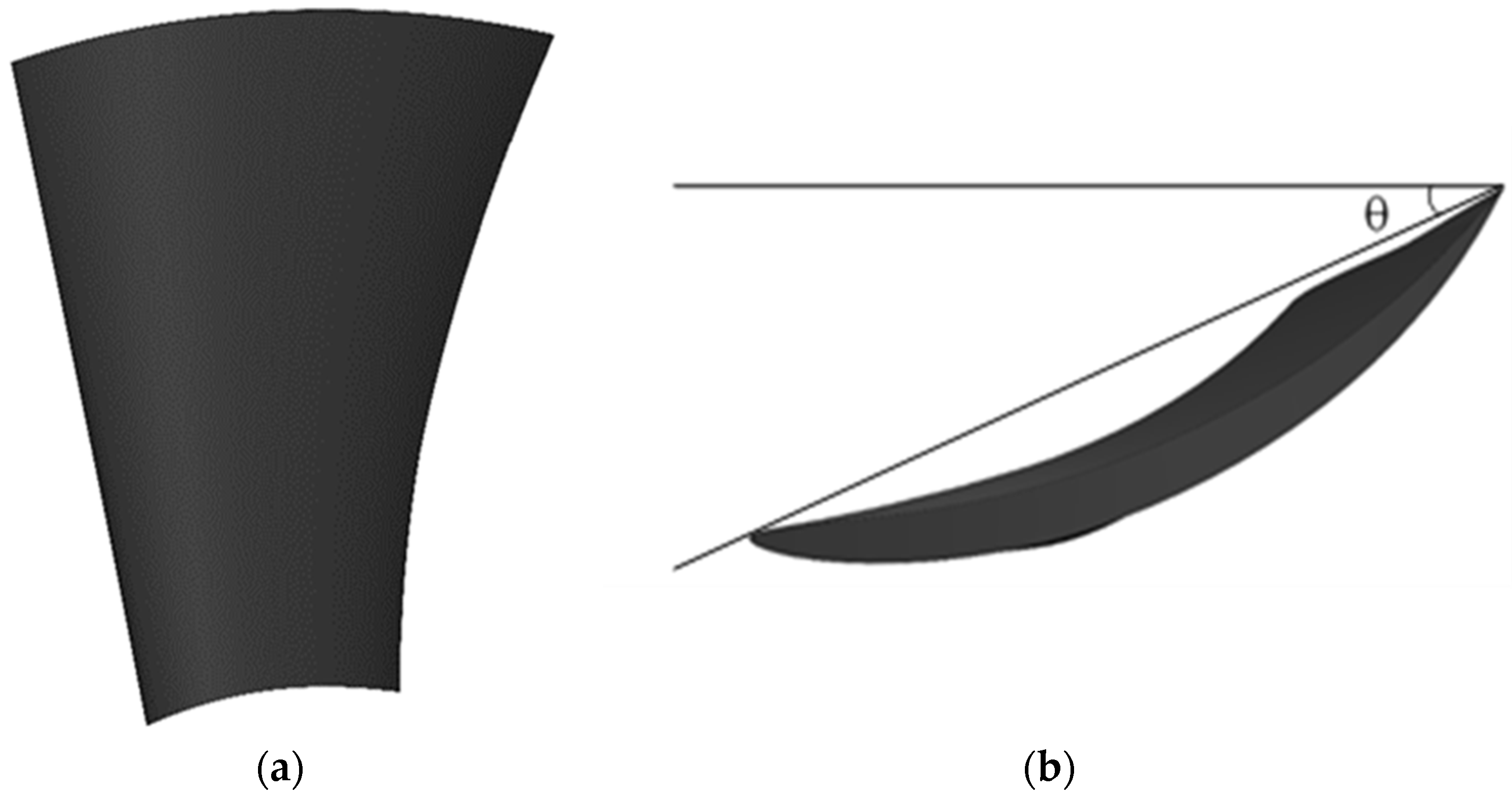
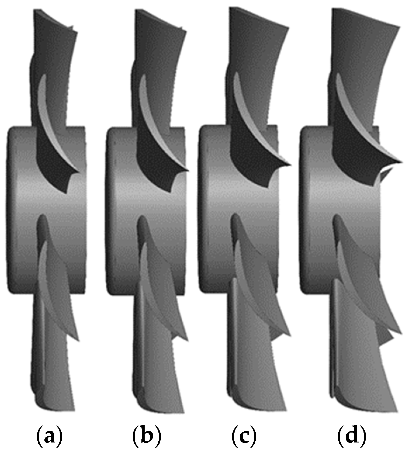
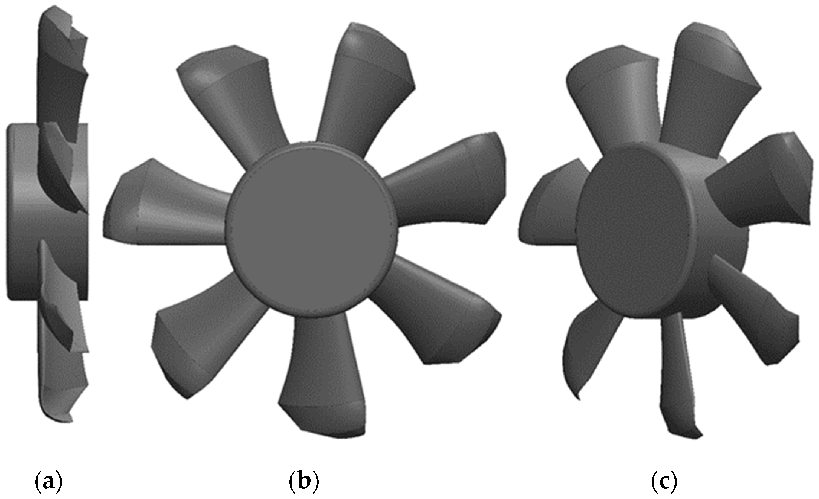
2.2. Blade Model Design

A step-wise geometry construction process is proposed here in the context of the blade design improvement of a small axial-flow fan rotor to enhance the fan design efficiency. In the first stage of the geometry construction, a baseline blade model with a 0° stagger angle and no winglet is generated using 10 segments identified with different NACA airfoil profiles in accordance with the experimental data available in the open literature [3]. The geometry specification of each blade segment, which is properly configured with a particular setting angle and chord length at each radial location to achieve a suitable angle of attack along the span of the 3-D blade, is listed in Table 1.
The generated seven-bladed baseline rotor geometry with a rotor diameter of 120 mm and a hub diameter of 50 mm is shown in Figure 1. This geometry, which has a twisted shape due to decreasing the setting angle from the hub to the tip, was also previously determined using the integrated design scheme through combining the cascade theory and an inverse design method for small-scale axial-flow fans [3].
In the second stage, having generated the baseline blade model, additional stagger angle adjustment is imposed on the baseline blade geometry while the chord length and the blade height remain the same (a solid rotation to all ten blade segments is imposed while the segment profile remains the same). The stagger angle is the angle between the chord line and the fan’s axial-flow direction of the blade (from hub to tip) and is denoted as θ as shown in Figure 2 which illustrates the schematic twisted contours of the blade. At this stage, each staggered blade model is designed having a specified non-varying stagger angle along the span of the blade. The newly generated three-rotor models having staggered blades of an additional +5°, +10°, or +15° degrees are shown in comparison with the baseline rotor model in Figure 3.
In the third stage, having determined the proper stagger angle for the blade geometry based on the fan’s design efficiency through the steady-state simulations performed under the design conditions, a winglet is designed with different values of the most aerodynamically effective geometrical parameters and is appended at the tip of the final staggered blade with the same chord and blade length. The same blade profile is also maintained for each winglet installation for the constant swept area of the rotor geometry.
The principal winglet design parameters which may affect the aerodynamic performance of the axial-flow fan blade are chosen in accordance with those of the study of Zhang et al. [30] and are depicted in Figure 4. Different winglet configurations are generated in accordance with the specified values of twist angle and curvature radius which are considered to be the most effective geometric parameters for the winglet design [29,31] while the winglet height and the tip chord length remain the same. In the winglet design, five different curvature radii and five different twist angles are used at the same winglet height of 10 mm and tip length of 10 mm. A total of twenty-five different wingletted blades are designed. The range of curvature radius values is decided according to the literature [29] and applied to the design. Previous studies [29,30] are taken into account while determining the pertinent twist angle range. The five different curvature radii are 6.77 mm, 7.10 mm, 7.30 mm, 9.77 mm, and 12.67 mm. All the winglets curve to the pressure side of the blade and 0°, 7°, 14°, −7°, and −14° twist angles are applied for each curvature radius value. Figure 5 also shows a generated rotor geometry which has seven staggered blades with winglets appended.

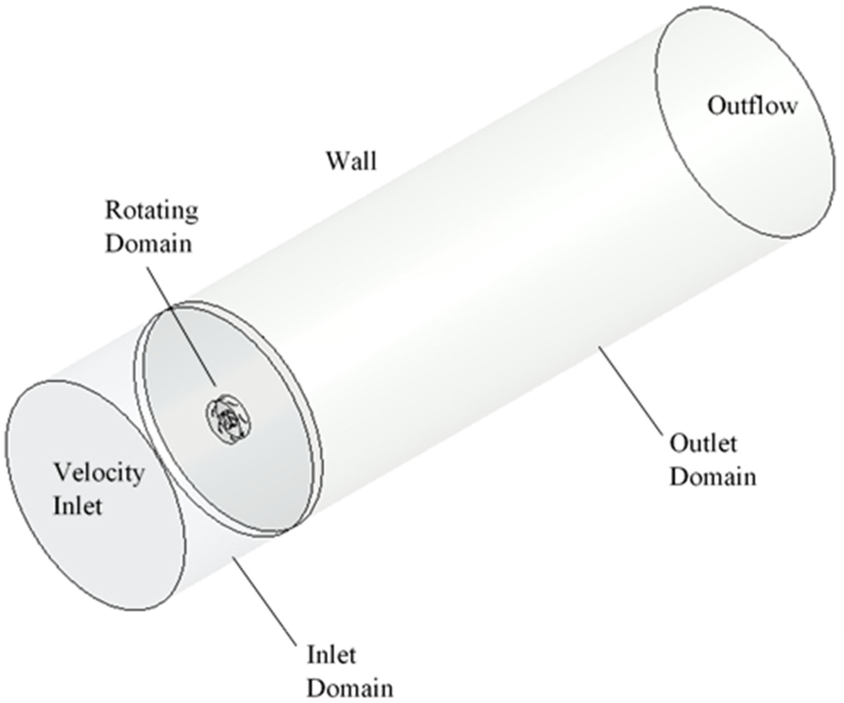
2.3. Computational Domain and Boundary Conditions

A large cylindrical flow domain, which comprises three sub-domains, namely, inlet sub-domain, rotating sub-domain, and outlet sub-domain, is constructed as shown in Figure 6. The inlet and outlet sub-domains are considered to be stationary flow domains with 500 mm and 2000 mm lengths, respectively, with the same diameter of 700 mm. The rotating sub-domain having a rotor geometry at the coordinate system’s origin with a diameter of 134 mm and a length of 35 mm is connected to both the inner sub-domain and outer sub-domain through the conformal interface boundary. The dimensions of the computational flow domain which are comparable with those of the experimental study [3] are set to very large values to minimize the effect of blockage and outlet reverse flow on the flow field.
The 3-D global and 2-D local computational mesh layouts employed for the full-scale model simulations are represented in Figure 7. The computational domain is constructed of unstructured tetrahedral mesh cells with very fine resolution in the close vicinity of the rotor surface as shown in Figure 7b,c. Due to the geometry complexity of the staggered blades with the winglets, the unstructured tetrahedral meshing approach with a patch-conforming algorithm is utilized in the entire computational domain. Additionally, a technique for a user-defined multi-block topology generation meshing method, which becomes more complex with a high stagger angle and winglet, is used. In this technique, instead of meshing a single block, the body is split from critical points into blocks; thereby, local meshing is used.
The rotor surface then comprises 32 different sub-faces for the wingletted fan. A high-resolution inflated boundary layer mesh accompanied with enhanced wall function is utilized around the rotor surface (Figure 7c) to accurately resolve the turbulent boundary layer and also to account for its separation under very high velocity and pressure gradients. Comparatively, coarse mesh resolution is employed in the inner and outer sub-domains except for their intersections with the rotating sub-domain where a conformal interface zone with very high mesh resolution is generated. Due to the geometry complexity of the blade shapes with the winglets, special attention is required around the tip of the blades and winglets where unstructured local mesh with a higher number of mesh cells is employed. While constructing both global and local mesh structures/configurations, various quality parameters including aspect ratio, skewness, orthogonal quality, and local cell Reynolds number, i.e., y+, are taken into account. The conformal interface boundary condition is applied at the interfaces between the stationary sub-domains, i.e., inlet and outlet sub-domains, and the rotating sub-domain for the MRF mesh interface approach. A velocity inlet boundary condition is imposed at the inlet boundary of the computational domain and the required velocity value which is normal to the boundary is computed using a specified volumetric flow rate value. Further, the outflow boundary condition is imposed at the outlet boundary to satisfy the fully developed flow condition. Diffusion fluxes for all flow variables in the direction normal to the outlet boundary are assumed to be zero. Therefore, outflow velocity and pressure are consistent with a fully developed flow assumption. A free-slip boundary condition is assigned to the outer cylindrical wall surface of the computational domain. The normal velocity components and the normal gradients of all velocity components are assumed to be zero there. The no-slip velocity boundary condition is adopted on the rotor surfaces to satisfy the zero relative velocity with respect to the rotating sub-domain which rotates at a specified constant rotational speed of 2000 rpm in accordance with the experimental data.

2.4. Fluid Flow Solver

A finite volume method (FVM)-based fluid flow solver [33] is employed for RANS-equation-based turbulence model simulations of highly 3-D, viscous, and turbulent airflow around the full-scale rotor geometry. A multiple rotating reference frame (MRF) approach is used to couple the rotating and stationary flow zones for steady-state flow analysis with additional source terms included in the RANS equations in design and off-design conditions over a large range of volumetric flow rate at a specified rotational speed of 2000 rpm in accordance with the experimental data [3]. The double-precision pressure-based segregated solver algorithm is used to solve the governing flow equations and the transport equations of turbulence scalars in a sequential manner for both steady and unsteady modes and the second-order upwind scheme is used for both spatial and temporal discretization. In addition, the semi-implicit pressure-linked equations (SIMPLE) algorithm is used as a pressure–velocity coupling scheme to accelerate the convergence of the simulations. The solution is considered to be converged when the difference between successive iterations for each flow solution parameter is less than 10−4. The simulations are performed on a 16-processor Intel Xeon® CPU E5-2690 v4 2.6 GHz high-performance computer (HPC) with 128 GB RAM per unit (Intel, Santa Clara, CA, USA).

3. Results and Discussion

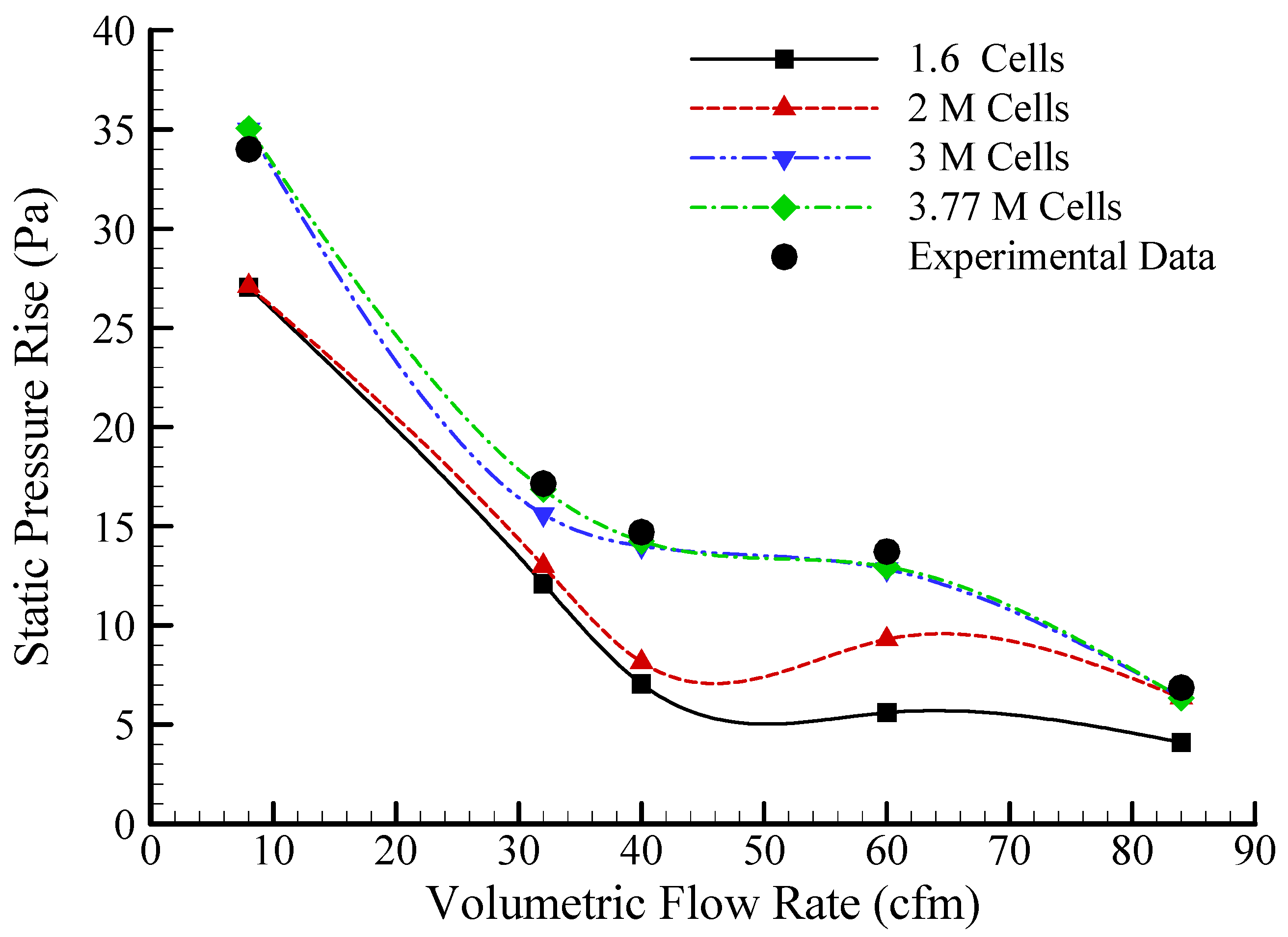
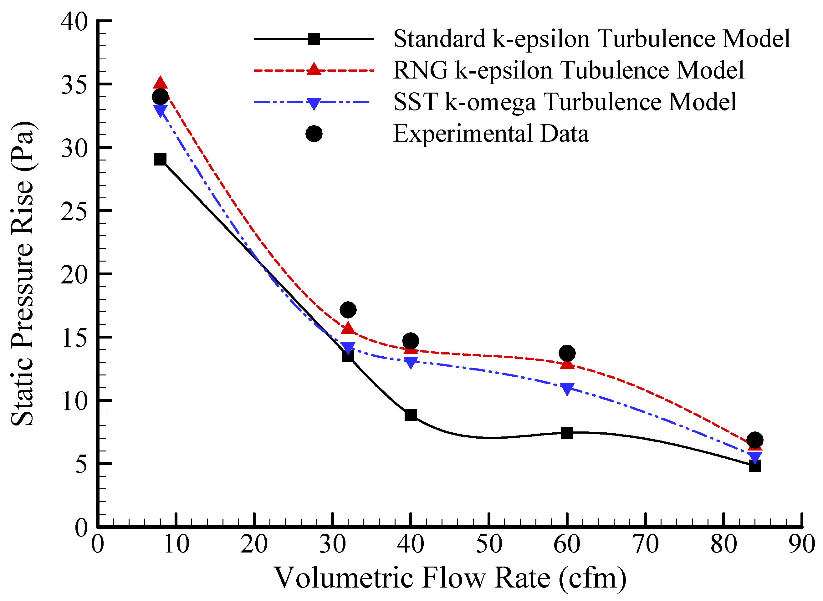
3.1. Model Validation

The proposed computational modeling approach is validated against the experimental data of Lin and Tsai [3] for the baseline rotor geometry in terms of the performance characteristic curve which is called the static pressure–volumetric flow rate performance curve (PQ curve). Before validating the accuracy of the RANS-equation-based turbulence models, a mesh independency study is conducted under different volumetric flow rates at a constant rotational speed of 2000 rpm to demonstrate the sensitivity of the simulation results to the number of volume cells and hence to determine the optimum mesh resolution within the fluid flow domain and the near-wall boundaries of the rotor surface. For this, four different mesh systems containing 1,600,000 (M1), 2,000,000 (M2), 3,000,000 (M3), and 3,770,000 (M4) unstructured tetrahedral volume cells, respectively, are employed with enhanced wall function by maintaining the y+ values in the acceptable prescribed range (y+ < 5). Table 2 summarizes the statistical details of the mesh systems employed for the mesh independency test.
The RNG kε turbulence model with a rotation correction is initially selected for simulating the flow through the MRF interface approach. The RNG kε turbulence model differs from the standard kε turbulence model by the inclusion of an additional sink term in the turbulence dissipation equation to account for non-equilibrium strain rates and employs different values for the various model coefficients. Previous computational studies performed on axial-flow fans and turbines demonstrate that the RNG kε turbulence model resolves the rotating flow, boundary layer separation under an adverse pressure gradient well [16,22,23,24]. The RNG kε turbulence model with enhanced wall treatment is integrated down to the solid boundaries (i.e., hub fan and the blades) where the first computational cell center is placed in the range of 0.1 < y+ < 5. This enhanced wall treatment which combines a two-layer model with so-called enhanced wall functions when applied with a swirl option (as we utilize in the present study) guarantees the correct asymptotic behavior for large and small values of y+ and reasonable representation of velocity profiles in the cases where y+ falls inside the wall buffer region (3 < y+ < 10) [33].
The predicted static pressure rise versus flow rate (ΔPsQ) curve is compared with the experimental data for each mesh system as seen in Figure 8. The static pressure and the flow rate are considered to be primary parameters which govern the fan performance. The proposed modeling approach simulates the evolution characteristic well, i.e., the tendency of the static pressure rise across the axial-flow rotor fan for each mesh resolution at the same rotational speed of 2000 rpm except with lower mesh resolutions. The static pressure rise decreases rapidly with increasing flow rate until 40 cfm in the deep-stall regime, followed by a small flow rate range, i.e., “stall range” (flow rate ranging between 40 cfm and 60 cfm) through which the decrease rate of the pressure rise becomes significantly retarded with the increase in the flow rate up to a local peak point signifying the end of the stall regime. After the stalling range (Q > 60 cfm), the pressure difference starts to decrease in all cases, and then the fan can no longer work efficiently. This regime is called the “pre-stall regime”.
As depicted in Figure 8, simulations performed with lower mesh resolutions, namely, M1 and M2, significantly underpredict the experimental ΔPsQ curve and reproduce much lower pressure rise values compared with those performed with higher mesh resolutions, namely, M3 and M4. Therefore, the correspondence with the experimental data is much better for higher mesh resolutions and even no discernable pressure difference is observed between the experimental and the simulation data for M3 and M4 over a large range of volumetric flow rate. The average relative deviation of the static pressure rise within the selected volumetric flow rate range of 60–80 cfm is 2.0 and 1.5 percent for M3 and M4, respectively. The resolution of mesh system of 3,000,000 (3,071,663) volume cells in which the inlet sub-domain is divided into 774,176 volume cells, the outlet sub-domains into 797,433, and the rotating sub-domain into a total of 1,500,054 is chosen as an optimal mesh resolution to provide the required spatial resolution without compromising between the computational cost and accuracy of the modeling approach. This mesh resolution is adopted for a further turbulence modeling accuracy test and comparative design performance study.
The accuracy of the proposed computational modeling approach is further assessed through different turbulence model simulations which are conducted with varying volumetric flow rate at the rotational speed of 2000 rpm for the chosen optimal mesh resolution of 3,000,000 tetrahedral volume cells. The 3-D RANS-equation-based turbulence models, namely, the standard kε model, the RNG kε model, and the transition SST kω model, are utilized for this purpose. The computed fan performance curve (ΔPsQ) is comparatively presented for each turbulence model simulation in Figure 9. The corresponding experimental data of Lin and Tsai [3] are also included in the figure for a direct comparison. As seen in the figure, though each turbulence model simulation reproduces the pressure rise tendency well over a large range of volumetric flow rate in accordance with the experimental data, a better correspondence with the experimental data is found with the RNG kε turbulence model simulation. Therefore, the RNG kε turbulence model is chosen as a more suitable turbulence model than the other turbulence models to simulate the rotational flow field around the rotor blades through their optimization process. In the present study, it is really difficult to maintain the local cell Reynolds number requirement along the entire solid surfaces under y+ of 1 due to the large scale ratio of the rotor body and the winglet. The SST kω turbulence model therefore may not produce more accurate results in terms of the static pressure rise across the rotor compared to the RNG kω turbulence model.
Recent numerical studies continue to verify the feasibility of applying standard kε and RNG kε turbulence models [22,34] and the SST kω turbulence model [20,35,36] under a steady-state flow assumption while the unsteady Reynolds-averaged Navier–Stokes (URANS) SST kω turbulence model [37], LES turbulence model [38], and hybrid URANS-LES turbulence model [39] are alternatively adopted successfully under an unsteady flow assumption depending on the complexity of the rotating flow and boundary layer separation under an adverse pressure gradient.

3.2. The Effect of Design Parameters

A parametric study of the individual or combined effect of stagger angle and winglet on the fan performance is conducted and both qualitative and quantitative analyses of the results are presented in a comparative manner in the name of determining the best possible blade design for the investigated design parameters. Table 3 summarizes the results of all design cases, which are simulated using the RANS-based RNG kε turbulence model in conjunction with the MRF technique, for a design flow rate of the baseline rotor geometry (Q = 60 cfm) at a rotational speed of 2000 rpm. Table 3 clearly demonstrates that an additional stagger angle implemented in the baseline blade model (case 1) significantly affects the performance and the best total efficiency value of 42.30 percent for a staggered blade without a winglet is predicted for the case of a stagger angle of +10° (case 3).
Having computed the area-weighted average total pressure at a specified flow rate and the shaft power, the total efficiency of the fan,   η can be determined as follows:
η = P t Q I P
where P t   is the area-weighted average total pressure difference between the axial fan’s outlet and inlet, Q is the volumetric flow rate, and I P is the shaft power. Taking advantage of the relationship between torque and the moment coefficient, total efficiency, η is explicitly calculated using the generated simulation data as follows:
η = P t Q 1 2 ρ V 2 A R C m ω
where ρ is the fluid density, V is the air inflow velocity, A and R are the projected area of the axial-flow fan and its radius, respectively, and ω is the rotational speed of the rotor.
As identified in Table 3, the use of a stagger angle does not directly enhance the fan performance as observed in cases of +5° and +15° stagger angles. Further design optimization with the installation of the winglet at the tip of the blade with varying values of the characteristic parameters is accomplished and the best total efficiency value of 43.80 percent is obtained when a winglet with a curvature radius of 6.77 mm and a twist angle of −7° is installed on the tip of the staggered blade of +10° (case 8). Similar fan performance behavior for the winglet use may also be observed so that installation of a winglet on the tip of the final blade with the stagger angle of +10° affects the fan efficiency with different degrees (either positive or negative influence of the winglet on the efficiency is observed). Nevertheless, the final blade design (case 8) significantly improves the total fan efficiency in the design condition when compared to the original baseline model operating at the same design flow rate of 60 cfm. The off-design performance of the fan is later studied through selected design cases over a large range of flow rates.

3.2.1. Fan Performance Curves

The fan performance curves obtained from different stagger angle cases without winglets (cases 1–4) are comparatively presented in Figure 10a–c in terms of the static pressure rise–volumetric flow rate (ΔPsQ) curve, the shaft power–volumetric flow rate (IPQ) curve, and total efficiency–flow rate (ηQ) curve, respectively. It is clearly seen in Figure 10a that the use of an additional stagger angle significantly influences the evolution of static pressure rise which represents three characteristic regimes, namely, deep-stall regime between a flow rate of 8 cfm and 40 cfm, stall regime between a flow rate of 40 cfm and 60 cfm, and pre-stall regime between a flow rate of 60 cfm and 84 cfm. A considerably higher pressure rise is obtained for a stagger angle of +10° (case 3) than that of other cases for the volumetric flow rate ranging from 50 cfm to 84 cfm in the mid-stall and pre-stall regimes where an approximately 10–15 percent higher pressure rise is predicted for case 3 than that of the baseline rotor blade. In the deep-stall regime, a stagger blade with an angle of +5° (case 2) is identified as the worst design case while a +15° staggered blade is the best design case. However, the fan performance for the latter case significantly decreases due to the stall of the rotor around 50 cfm and the best fan performance is therefore predicted by a stagger angle of +10° with a flow rate of 50 cfm. The power–flow rate curve in Figure 10b represents the variation tendency of the fan power input, i.e., power consumption of the fan. It is clearly seen in the figure that the fan power input is highly dependent on the stagger angle and a staggered angle of +5° requires the maximum power input while a stagger blade angle of +10° requires the minimum one over the whole operation range. It is also seen in Figure 10c that the best efficiency point (BEP) for the baseline geometry corresponds to a flow rate of 60 cfm and the use of different additional stagger angles shifts the BEP for the flow rate ranging from 55 cfm to 65 cfm. As expected, the efficiency of each case first increases up to a certain volumetric flow rate and then decreases sharply after the BEP. Very similar efficiency characteristics are obtained for each case except the case of a +10° stagger angle, which provides a large deviation from the other cases with lower efficiency values at lower flow rates up to an off-design flow rate of 40 cfm. A stagger angle of +10° case reproduces a much higher fan static pressure rise as well as a lower fan power input, which results in much higher total efficiency values with a flow rate of 40 cfm and the BEP corresponds to a flow rate of 65 cfm (higher than those of other cases) with a total efficiency value of 42.8 percent.
When compared to the baseline model operating in a design condition of Q = 60 cfm, it is clearly observed that the +10° staggered blade case predicts a total efficiency of 42.3 percent which is much higher than those of other stagger angle cases which predict 29.3 and 31.3 percent for +5° and +15°, respectively. Therefore, an additional stagger angle of +10° is considered to be the most suitable staggered blade angle around the design condition of Q = 60 cfm at N = 2000 rpm.
Further design improvement with the installation of a winglet at the blade tip of a +10° stagger angle with different characteristic design parameters also suggests that different total efficiency curves are predicted as illustrated in Figure 11. The efficiency curves of the baseline blade model and the staggered angle of +10° are also included in the figure for comparison.
The best efficiency distribution is reproduced for the winglet with a curvature radius of 6.77 mm and a twist angle of −7° (case 8) for which the BEP corresponds to a flow rate of 60 cfm with a total efficiency of 43.8. Nevertheless, considering the total performance of the fan throughout the whole operation range, i.e., volumetric flow rates, a winglet which is installed at the tip of a stagger blade of +10° degrees with a curvature radius of 6.77 mm and a twist angle of −7° represents the best performance among all the cases assessed.

3.2.2. Pressure Contours

The external near-body flow characteristics of a small-scale axial-flow fan can be considered to be the key factor that affects its aerodynamic performance [14] so comparative representation of total pressure and velocity vector fields around the fan blades can be a very useful approach for qualitative analysis of the flow field for determining the best possible performance of the fan. In this respect, Figure 12 and Figure 13 illustrate the total pressure contours and the streamlines colored by relative axial velocity magnitudes of the meridional plane of the fan, respectively, for selected cases at a design volumetric flow rate of 60 cfm for the baseline geometry. As clearly seen in Figure 12a–f, there is a noticeable total pressure increase across the fan as an additional pressure head delivered to the fluid flow (fluid work input) due to rotational motion of the blades and adjustment of different stagger angles and/or winglets has a noticeable effect on the total pressure distribution at the fan exit and in the vicinity of the blade tips while very similar pressure contours with stagnation conditions are predicted in the inlet region of the fan. On the other hand, more discernible and locally higher total pressure contours around the rotor blades appear to be distributed towards the tip of the blades and this can be attributed to the predominant effect of rotational or tangential forces over the axial forces which may be considered to be the main driving forces for the development of the downstream flow rate.
Nevertheless, the higher total pressure rise, which is extended in a larger zone at the exit of the fan and near the tip blade region for the +10 degree staggered blade without a winglet, signifies that higher total efficiency is attained for this case compared to other staggered blades without a winglet as depicted in Figure 12c. Winglet installation further develops the total pressure distribution at the fan exit and near the blade tips by possibly preventing excessive tip leakage flow and better rotational periodicity of the total pressure distribution with respect to the centerline of the rotor geometry in the near-wake region of the fan occurs as clearly observed in Figure 12e,f.

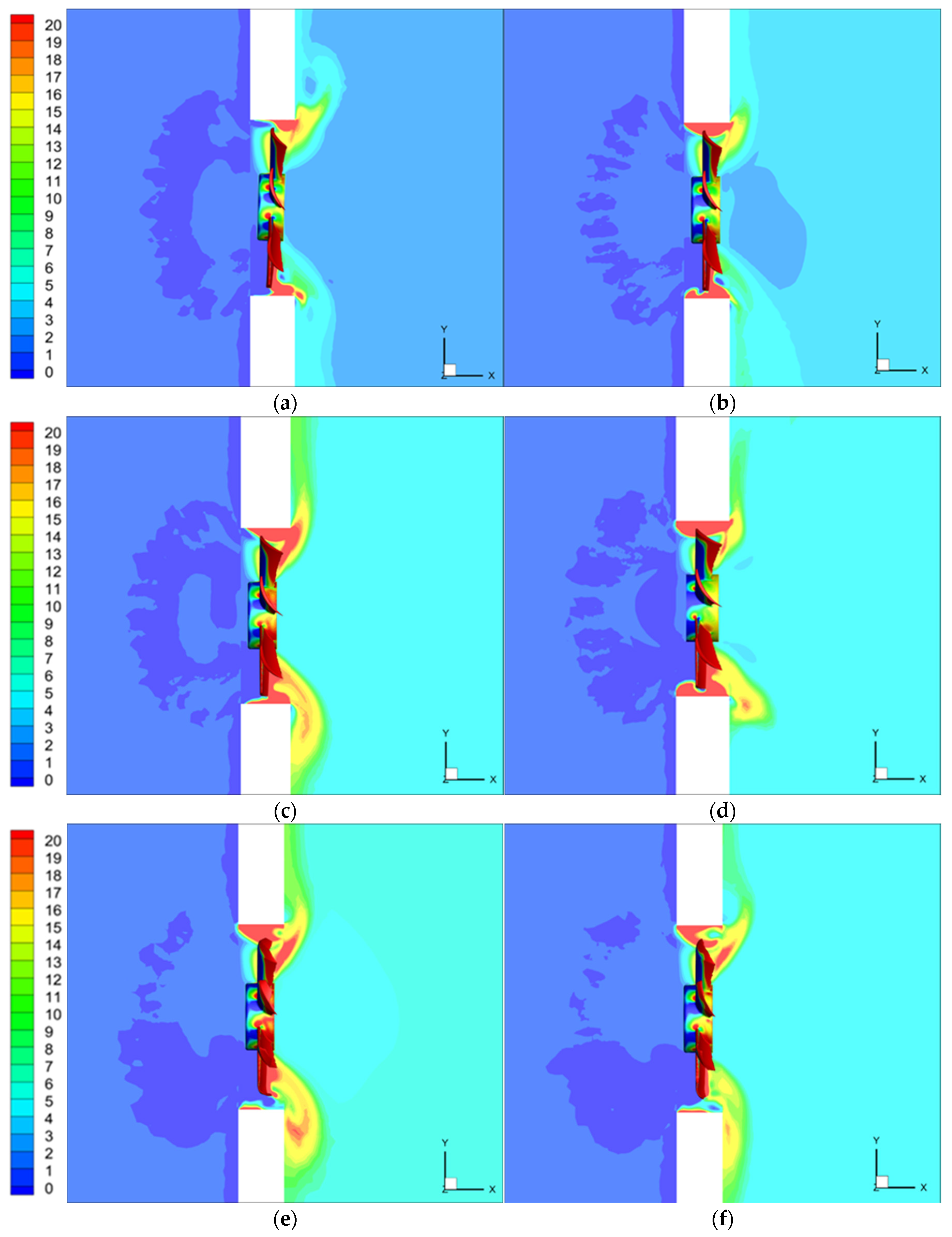
3.2.3. Streamlines and Velocity Contours

Figure 13a–f illustrate the velocity streamlines and the axial velocity contours of the meridional plane of the fan. It can be seen that a nearly uniform flow field is reproduced upstream of the fan for each case while the flow field downstream of the fan changes significantly with varying blade profile. The relative velocity near the exit of the blades presents larger axial velocity components as an indication of increasing dynamic pressure (i.e., velocity pressure). The primary boundary layer separation from the suction surface of the blades leads to the formation of a recirculation zone with varying degrees of size, location, and extent depending on the blade configuration. A pair of almost symmetrical, very large, and more developed recirculation zones behind the fan is formed for the baseline model. With increasing stagger angle, these recirculation zones present a more developed and asymmetrical character than those observed for the baseline model and strongly interact with each other while decreasing in size and moving away from the fan surface. The development of asymmetric behavior of downstream flow suggests that a time-dependent flow field is required to be computed as transient features dominate [40]. For such cases, transient techniques such as a sliding mesh (SM) model can be utilized in computations [40].
With the installation of the winglet at the tip of the +10° staggered blade, the formation behavior of the recirculation zones alters again and becomes slightly more elongated and almost symmetrical and the developed recirculation zones are reproduced downstream of the fan. A broader and more uniform flow field in the immediate wake region of the fan is also identified for the wingletted blade models as an indication of a higher total pressure rise. The variation in the formation of the recirculation zone depending on the blade configuration directly affects the near-wake total pressure distribution and hence the fan performance, i.e., there is a certain relationship between the performance characteristic of the fan and the downstream flow field development.

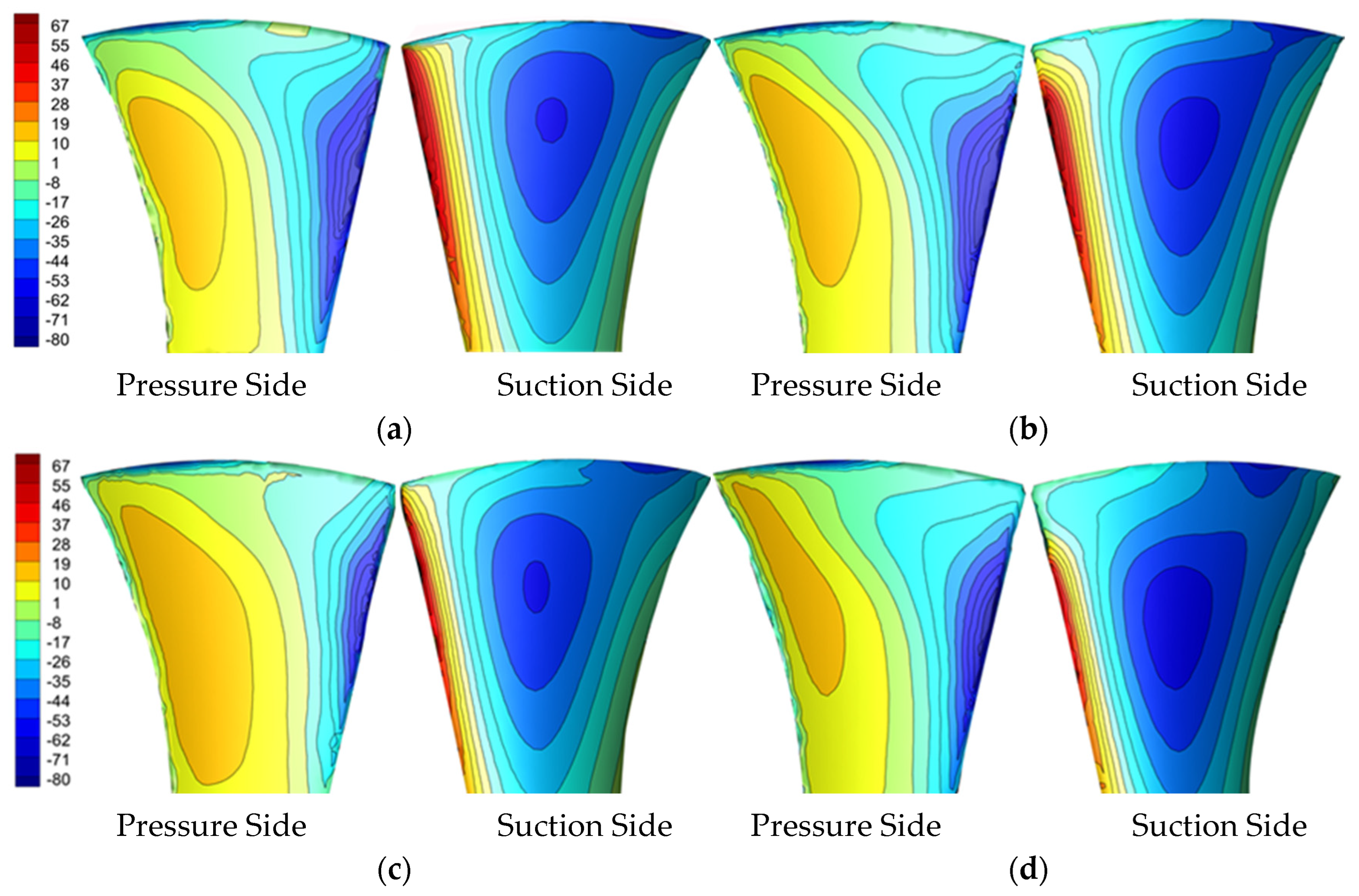
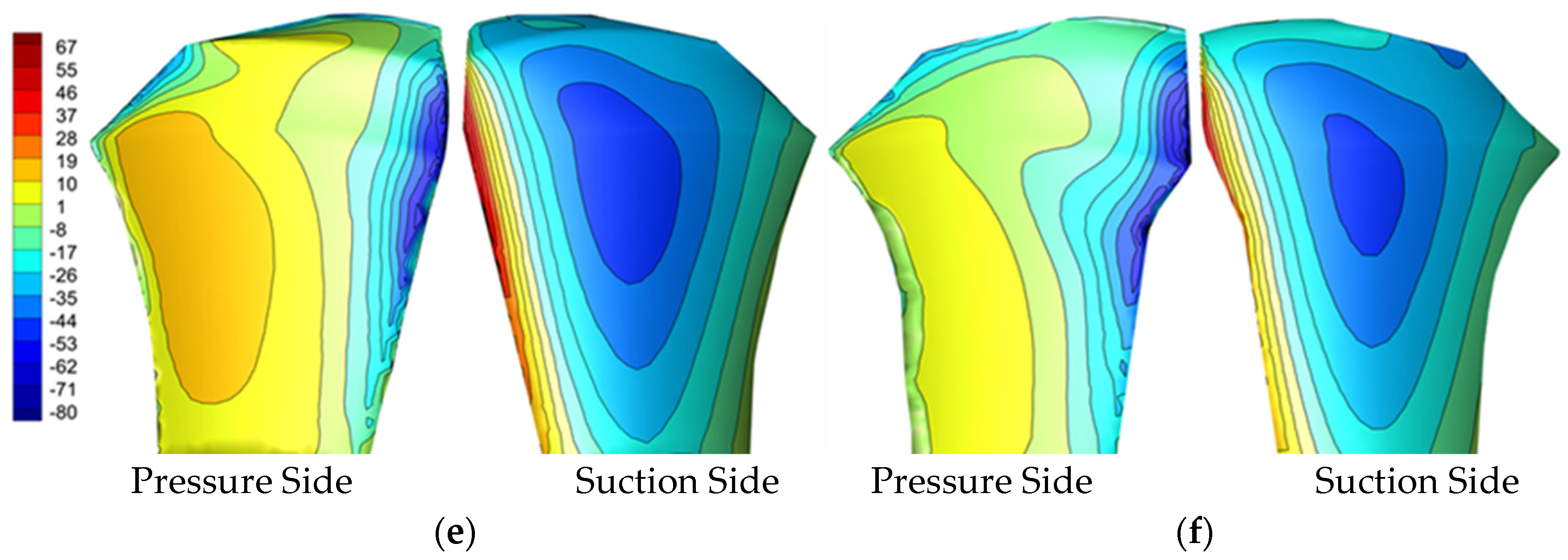
3.2.4. Suction and Pressure Side Pressure Contours

Further qualitative analysis of the results is accomplished in terms of the static pressure contour distribution of the suction and pressure surfaces of the fan blade when the fan operates at s design volumetric flow rate of 60 cfm and rotational speed of 2000 rpm. As seen in Figure 14a–f, a lower pressure region is identified on the suction surface and a higher pressure region on the pressure surface of each blade model. The maximum pressure distribution is identified at the leading edge of the suction surface while the lower pressure distribution is concentrated towards the trailing edge for both surfaces. Though similar pressure distributions are found on each surface of the blade for each case, the high-pressure region on the pressure surface extends more for case 8 compared to that of other cases as depicted in Figure 14e due to a slight adjustment of local flow direction. This signifies that the blade pressure difference of a +10° staggered blade with a winglet installed at the tip of the blade with a curvature radius of 6.77 mm and a twist angle of −7° is greater than that of other blade models. This larger pressure difference contributes more to the total pressure difference across the fan and hence the enhancement in the total efficiency of the fan for this case.

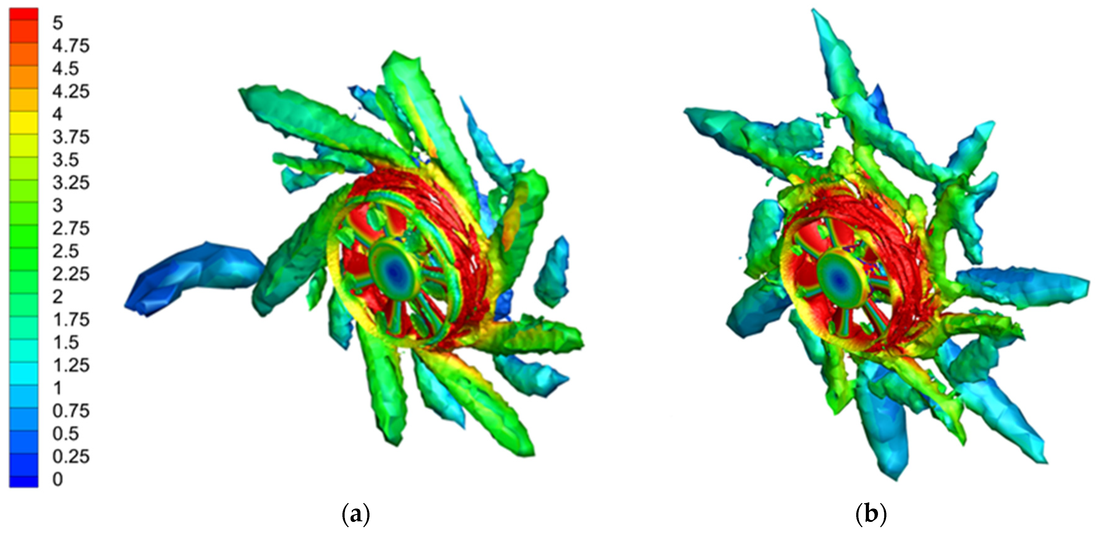
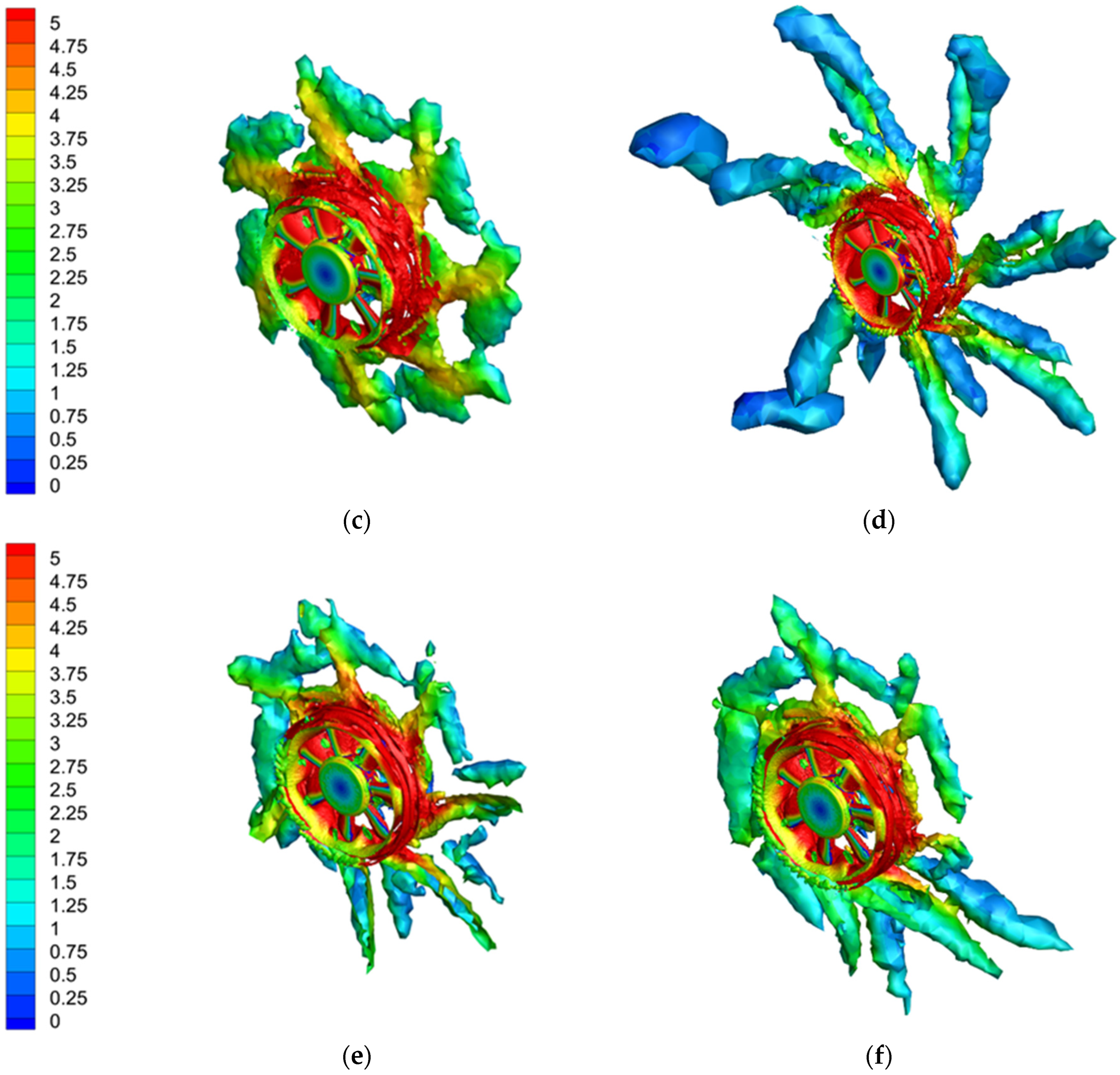
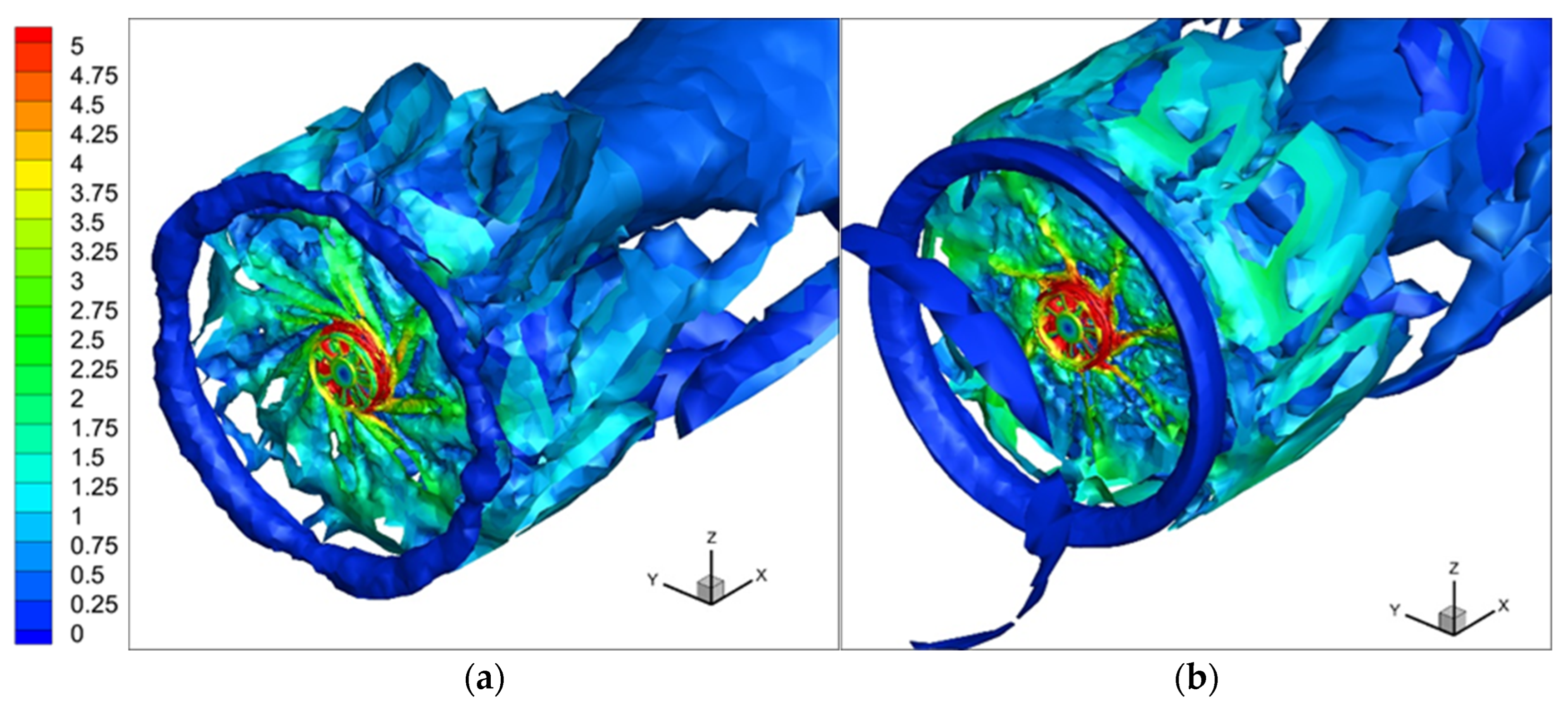
3.2.5. Q–Criterion Contours

The Q–criterion colored by velocity magnitude contours provides further information on the near flow field characteristics associated with the vorticity distributions and the velocity magnitude as illustrated in Figure 15a–f. The Q–criterion represents a technique for the identification of the vortical structures in the flow field, as the region where the second invariant of the velocity gradient tensor is positive. Figure 15a–e clearly represent the complexity of the flow surrounding the rotor surface and the vortical structures generated by the rotational flow at the tip of the blades from which a vortex shedding is clearly depicted for each case.
The unsteadiness of the near-wake flow can be attributed to the occurrence of these structures. It is also seen from the figures that the vorticity distributions at the tip of the staggered blade with a winglet are slightly weaker and more uniform than those of the baseline blade and the staggered blade without a winglet. The smoother vorticity gradient variation from the tip of the blades with winglets leads to more uniform flow development in the near wake of the fan as previously illustrated from the streamline contours, which in turn improves the aerodynamic performance of the near region of the blade tips as expected.
The development of the vortices in the near-wake flow region can also be seen in Figure 16a,b for the baseline blade and the +10° staggered blade with a winglet. Both figures illustrate that the tip vortices of both rotor blades mix and separate in the very close proximity of the rear surface of the blades, then this mixing and separation process continues with a significant decrease in vorticity magnitude (less vorticity and weaker vortices are observed in the near-wake flow region).

4. Conclusions

Both individual and combined uses of blade stagger angles and winglets are proposed in the context of passive flow control techniques to enhance the aerodynamic performance of a small axial-flow fan in both design and off-design conditions using a computational fluid flow methodology. An eddy-viscosity-based RNG kε turbulence model coupled with the MRF technique is utilized for parametric simulations to comparatively analyze the total pressure rise across the fan and total fan efficiency together with the qualitative results in terms of near-body flow field distribution of the fan. Specific conclusions can be drawn from the present computational fluid flow simulations:
  • The stagger angle and winglet both have a significant influence on the performance characteristics of the small axial-flow fan. The total pressure rise across the fan and the total fan efficiency curve are both highly dependent on the stagger angle and the winglet which may have a positive or negative influence on the fan performance characteristics depending on the choice of values of these two parameters.
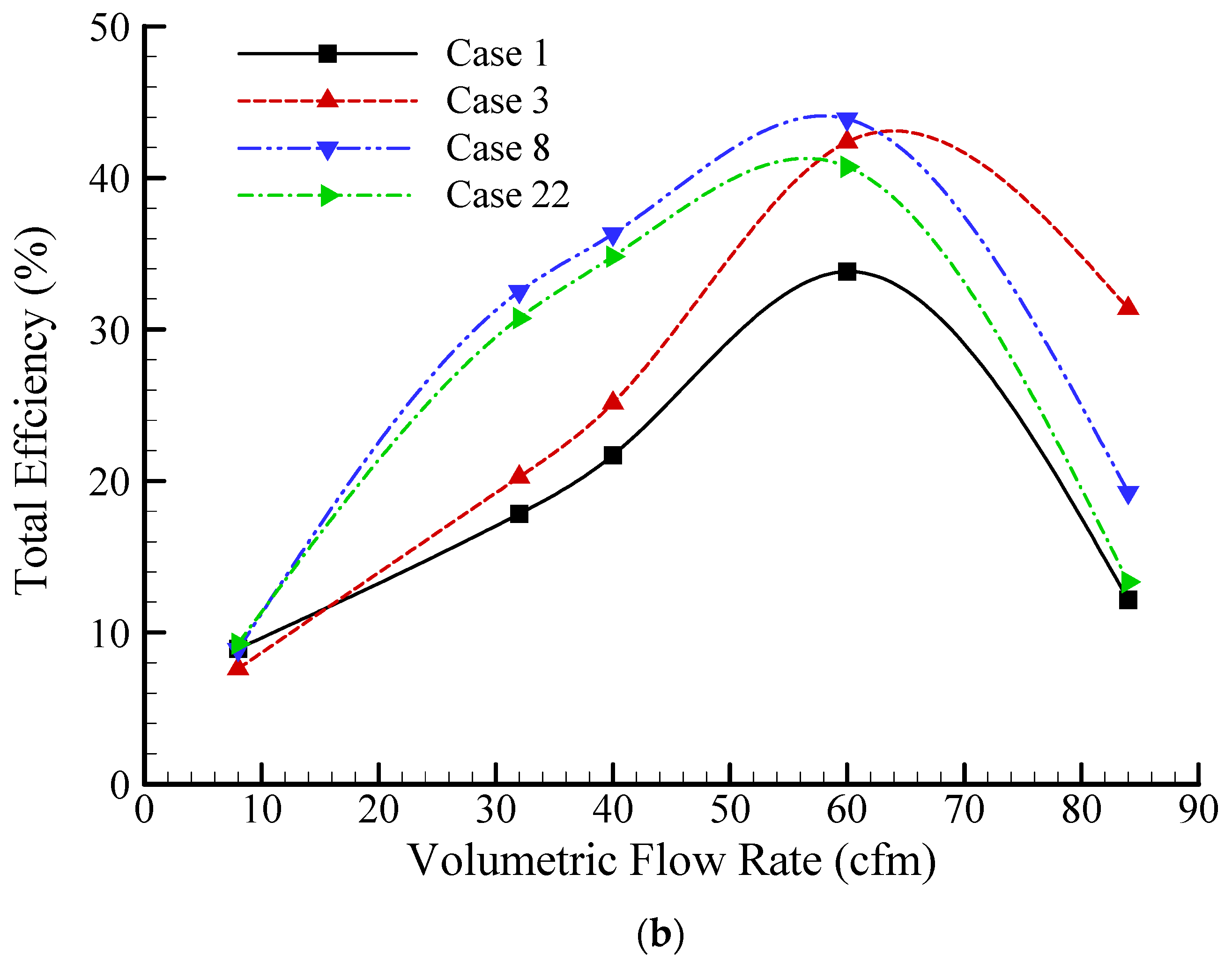
  • The fan performance can be significantly improved using a critical value of the stagger angle together with an implementation of the winglet on the tip of the rotor blade. Considering the total efficiency for the investigated operation range, the fan attains the best performance with an additional stagger angle of +10° and a winglet with a curvature radius of 6.77 mm and a twist angle of −7° for the investigated dimensioning range. In the stall region, all staggered blades with and without winglets reproduce better efficiency curves than that of the baseline blade.
  • The use of different additional stagger angles shifts the best efficiency point (BEP) for the flow rate ranging from 55 cfm to 65 cfm while the use of different winglet configurations does not alter the BEP which is found to be around 60 cfm as observed for the baseline blade geometry.
  • The present three-dimensional (3-D) Reynolds-averaged Navier–Stokes (RANS) equation-based RNG kε turbulence modeling approach coupled with the multiple reference frame (MRF) technique which adopts a multi-block topology generation meshing method successfully resolves the rotating flow around the fan. The computed results compare well with the experimental data and suggest that the present computational methodology can be used with confidence for such flow analysis.
  • The near-wake flow characteristics of the fan which are governed by the flow separation and associated vortical structures generated from the tip of the blade are significantly affected by the blade geometry. The variation in behavior of vortex shedding and the formation of the recirculation zone depending on the blade geometry directly affects the near-wake total pressure distribution and hence the fan performance. The wingletted blade better controls the flow in the very near-wake region of the fan.

Author Contributions

Conceptualization, M.T. and J.B.C.; methodology, M.T. and J.B.C.; software, J.B.C.; validation, J.B.C.; formal analysis, M.T.; investigation, M.T. and J.B.C.; resources, M.T.; data curation, M.T.; writing-original draft preparation, M.T. and J.B.C.; writing-review and editing, M.T. All authors have read and agreed to the published version of the manuscript.

Funding

This research received no external funding.

Institutional Review Board Statement

Not applicable.

Informed Consent Statement

Not applicable.

Data Availability Statement

Data will be available upon request.

Conflicts of Interest

The authors declare no conflicts of interest.

References

  1. Babu, A.M.; Gangadhar, V.V.R.L.S.; Reddy, A.C.S. Modeling and analysis of tube axial flow fan by comparison of material used and changing the number of blades. Int. J. Sci. Eng. Technol. Res. 2014, 3, 4730–4736. [Google Scholar]
  2. Dwivedi, D.; Dandotiya, D.S. CFD Analysis of axial flow fans with skewed blades. Int. J. Emerg. Technol. Adv. Eng. 2013, 3, 741–752. [Google Scholar]
  3. Lin, S.-C.; Tsai, M.-L. An integrated study of the design method for small axial-flow fans, based on the airfoil theory. Int. J. Adv. Eng. Innov. Technol. 2010, 225, 885–895. [Google Scholar] [CrossRef]
  4. Zhou, J.-H.; Yang, C.-X. Parametric design and numerical simulation of the axial-flow fan for electronic devices. IEEE Trans. on Comp. Pack. Technol. 2010, 33, 287–297. [Google Scholar] [CrossRef]
  5. Quin, D.; Grimes, R. The effect of Reynolds number on microaxial flow fan performance. J. Fluids Eng. 2008, 130, 101101. [Google Scholar] [CrossRef]
  6. Sahu, M.D.; Bartaria, V.N. Characteristic curve determination of the analyzed impellers in axial flow fan. Int. J. Appl. Eng. Technol. 2016, 4, 452–456. [Google Scholar]
  7. Yadav, A.; Pathak, M.; Sharman, P.K. Numerical analysis of aerofoil section of blade of axial flow fan at different angle of attack. Int. J. Adv. Res. Ideas Innov. Technol. 2017, 3, 63–74. [Google Scholar]
  8. Liu, S.H.; Huang, R.F.; Chen, L.J. Performance and inter-blade flow of axial flow fans with different blade angles of attack. J. Chin. Inst. Eng. 2011, 34, 141–153. [Google Scholar] [CrossRef]
  9. Izadi, M.J.; Falahat, A. Effect of blade angle of attack and hub to tip ratio on mass flow rate in an axial fan at a fixed rotational speed. In Proceedings of the ASME Fluids Engineering Division Summer Conference, Jacksonville, FL, USA, 10–14 August 2008. [Google Scholar] [CrossRef]
  10. Hirano, T.; Otaka, T.; Minorikawa, G. Study on optimum design method for small axial fan. In Proceedings of the 4th International Conference on Design Engineering and Science ICDES 2017, Aachen, Germany, 17–19 September 2017. [Google Scholar]
  11. Luo, D.; Huang, D.; Sun, X.; Chen, X.; Zheng, Z. A computational study on the performance improvement of low-speed axial flow fans with microplates. J. Appl. Fluid Mech. 2017, 10, 1537–1546. [Google Scholar] [CrossRef]
  12. Ye, X.; Ding, X.; Zhang, J.; Li, C. Numerical simulation of pressure pulsation and transient flow field in an axial flow fan. Energy 2017, 129, 185–200. [Google Scholar] [CrossRef]
  13. Zhang, L.; Jin, Y.; Dou, H.; Jin, Y. Numerical and experimental investigation on aerodynamic performance of small axial flow fan with hollow blade root. J. Therm. Sci. 2013, 22, 424–432. [Google Scholar] [CrossRef]
  14. Zhang, L.; Jin, Y. Effect of blade numbers on aerodynamic performance and noise of small axial flow fan. Adv. Mater. Res. 2011, 199–200, 796–900. [Google Scholar] [CrossRef]
  15. Mao, H.; Wang, Y.; Lin, P.; Jin, Y.; Setoguchi, T.; Kim, H.D. Influence of tip end-plate on noise of small axial fan. J. Therm. Sci. 2017, 26, 30–37. [Google Scholar] [CrossRef]
  16. Liu, Y.; Lin, Z.; Lin, P.; Jin, Y.; Setoguchi, T.; Kim, H.D. Effect of inlet guide vanes on the performance of small axial fan. J. Therm. Sci. 2017, 26, 504–513. [Google Scholar] [CrossRef]
  17. Moosania, M.; Zhou, C.; Hu, S. Effect of tip geometry on the performance of low-speed axial flow fan. Int. J. Ref. 2022, 134, 16–23. [Google Scholar] [CrossRef]
  18. Pretorius, J.P.; Erasmus, J.A. Effect of tip vortex reduction on air-cooled condenser axial flow fan performance: An experimental investigation. J. Turbomach. 2022, 144, 031001. [Google Scholar] [CrossRef]
  19. Dellacasagrande, M.; Canepa, E.; Cattanei, A.; Moradi, M. Characterization of unsteady leakage flow in an axial fan. Int. J. Turbomach. Propuls. Power 2023, 8, 34. [Google Scholar] [CrossRef]
  20. Yadegari, M.; Ommi, F.; Aliabadi, S.K.; Saboohi, Z. Reducing the aerodynamic noise of the axial flow fan with perforated surface. App. Acoust. 2023, 215, 109720. [Google Scholar] [CrossRef]
  21. Zhao, Y.; Xu, C.; Zheng, Z.; Hu, X.; Mao, Y. Experimental study of the parameter effects on the flow and noise characteristics for a contra-rotating axial fan. Front. Phys. 2023, 11, 1153380. [Google Scholar] [CrossRef]
  22. Masi, M.; Danieli, P.; Lazzaretto, A. Effect of solidity and aspect ratio on the aerodynamic performance of axial-flow fans with 0.2 hub-to-tip ratio. J. Turbomach. 2023, 145, 081008. [Google Scholar] [CrossRef]
  23. Zhang, L.; Jin, Y.; Jin, Y. Effect of tip flange on tip leakage flow of small axial flow fans. J. Therm. Sci. 2014, 23, 45–52. [Google Scholar] [CrossRef]
  24. Liu, Y.; Lin, Z.; Lin, P.; Jin, Y.; Setoguchi, T.; Kim, H.D. Effect of the uneven circumferential blade space on the performance of small axial flow fan. J. Therm. Sci. 2016, 25, 492–500. [Google Scholar] [CrossRef]
  25. Cavazzini, G.; Giacomel, F.; Ardizzon, G.; Casari, N.; Fadiga, E.; Pinelli, M.; Suman, A.; Montomoli, F. CFD-based optimization of scroll compressor design and uncertainty quantification of the performance under geometrical variations. Energy 2020, 209, 118382. [Google Scholar] [CrossRef]
  26. Bianchi, S.; Corsini, A.; Sheard, A.G.; Tortora, C. A critical review of stall control techniques in industrial fans. ISRN Mech. Eng. 2013, 2013, 526192. [Google Scholar] [CrossRef]
  27. Johansen, J.; Sørensen, N. Aerodynamic Investigation of Winglets on Wind Turbine Blades Using CFD; Report No. Riso-R-1543(EN); Riso National Laboratory: Roskilde, Denmark, 2006. [Google Scholar]
  28. Li, W. Research on the Actuation Technology of Variable Height and Cant Winglet. Ph.D. Thesis, Nanjing University of Aeronautics and Astronautics, Nanjing, China, 2012. [Google Scholar] [CrossRef]
  29. Saravanan, P.; Parammasivam, K.M.; Selvi Rajan, S. Experimental investigation on small horizontal axis wind turbine rotor using winglets. J. Appl. Sci. Eng. 2013, 16, 159–164. [Google Scholar] [CrossRef]
  30. Zhang, T.-T.; Elsakka, M.; Huang, W.; Wang, Z.-G.; Ingham, D.B.; Ma, L.; Pourkashanian, M. Winglet design for vertical axis wind turbines based on a design of experiment and CFD approach. Energy Convers. Manag. 2019, 195, 712–726. [Google Scholar] [CrossRef]
  31. Cai, X.; Zhang, Y.; Ding, W.X.; Bian, S.X. The aerodynamic performance of H-type Darrieus VAWT rotor with and without winglets: CFD simulations. Energy Sources Part A Recovery Util. Environ. Eff. 2024, 46, 2625–2636. [Google Scholar] [CrossRef]
  32. Dejene, G.; Ramayya, V.; Bekele, A. Investigation of NREL Phase VI wind turbine blade with different winglet configuration for performance augmentation. Int. J. Sustain. Energy 2024, 43, 2321622. [Google Scholar] [CrossRef]
  33. Ansys Fluent, Version 19.1, User’s Manual. Available online: https://www.ansys.com/products/fluids/ansys-fluent (accessed on 5 May 2018).
  34. Wang, Z.; Liu, J.; Wang, H.; Zhang, B.; Liu, W.; Ozdemir, E.D.; Aksel, M.H. Numerical and experimental investigation on the integrate performance of axial flow cooling fan and heat exchanger. Appl. Therm. Eng. 2024, 245, 122814. [Google Scholar] [CrossRef]
  35. Chen, F.; Zhu, G.; Xi, D.; Miao, B. Air volume flow rate optimization of the guide vanes in an axial flow fan based on DOE and CFD. Sci. Rep. 2023, 13, 4439. [Google Scholar] [CrossRef]
  36. Fakhari, S.M.; Mrad, H. Optimization of an axial-flow mine ventilation fan based on effects of design parameters. Results Eng. 2024, 21, 101662. [Google Scholar] [CrossRef]
  37. Amin, G.; Salunkhe, P.; Kini, C. Numerical analysis of a novel casing treatment in an axial flow fan. J. Propuls. Power 2024, 40, 818–832. [Google Scholar] [CrossRef]
  38. Song, Y.G.; Ryu, S.Y.; Cheong, C.; Lee, I. Improvement in flow and noise performances of small axial-flow fan for automotive fine dust sensor. J. Acoust. Soc. Korea 2023, 41, 7–15. [Google Scholar] [CrossRef]
  39. Hur, K.H.; Haider, B.A.; Sohn, C.H. Trailing edge serrations for noise control in axial-flow automotive cooling fans. Int. J. Aeroacoustics 2023, 22, 713–730. [Google Scholar] [CrossRef]
  40. Hashim, H.M.; Dogruoz, B.; Arik, M.; Parlak, M. An investigation into performance characteristics of an axial flow fan using CFD for electronic devices. In Proceedings of the ASME 2015 International Technical Conference and Exhibition on Packaging and Integration of Electronic and Photonic Microsystems InterPACK2015, San Francisco, CA, USA, 6–9 July 2015. [Google Scholar]
Figure 1. The baseline geometry model; (a) Front view; (b) Side view.
Ijtpp 10 00001 g001
Figure 2. Stagger angle details; (a) Blade model; (b) Stagger angle.
Ijtpp 10 00001 g002
Figure 3. Generated rotor geometry models with different additional stagger angles; (a) Baseline geometry with 0°; (b) +5°; (c) +10°; (d) +15°.
Ijtpp 10 00001 g003
Figure 4. Winglet design parameters; (a) Tip length, Ctip; (b) Curvature radius, RCR and winglet height, Hw; (c) Twist angle, σ.
Ijtpp 10 00001 g004
Figure 5. Improved geometry model with the use of stagger angle and winglet; (a) Side view; (b) Front view; (c) Perspective view.
Ijtpp 10 00001 g005
Figure 6. Computational domain of the axial-flow fan.
Ijtpp 10 00001 g006
Figure 7. Computational mesh details; (a) Global mesh domain; (b) Local mesh around the blade; (c) Surface mesh of the rotor blades.
Ijtpp 10 00001 g007
Figure 8. Mesh independency test in terms of static pressure rise vs. volumetric flow rate (ΔPsQ) curve.
Ijtpp 10 00001 g008
Figure 9. Turbulence modeling test for optimal mesh resolution chosen in terms of ΔPsQ curve.
Ijtpp 10 00001 g009
Figure 10. Performance curves of simulated design cases for different stagger angles without winglets appended; (a) ΔPsQ curve; (b) IPQ curve; (c) ηQ curve.
Ijtpp 10 00001 g010aIjtpp 10 00001 g010b
Figure 11. Comparison of fan performance curves from simulated selected design cases; (a) IPQ curve; (b) ηQ curve.
Ijtpp 10 00001 g011aIjtpp 10 00001 g011b
Figure 12. Total pressure contours obtained from selected design cases simulated at Q = 60 cfm and N = 2000 rpm; (a) Case 1; (b) Case 2; (c) Case 3; (d) Case 4; (e) Case 8; (f) Case 22.
Ijtpp 10 00001 g012
Figure 13. Streamline contours colored by axial velocity magnitude for selected design cases simulated at Q = 60 cfm and N = 2000 rpm; (a) Case 1; (b) Case 2; (c) Case 3; (d) Case 4; (e) Case 8; (f) Case 22.
Ijtpp 10 00001 g013
Figure 14. Static pressure contour for suction and pressure side of a chosen rotor blade for selected design cases simulated at Q = 60 cfm and N = 2000 rpm; (a) Case 1; (b) Case 2; (c) Case 3; (d) Case 4; (e) Case 8; (f) Case 22.
Ijtpp 10 00001 g014aIjtpp 10 00001 g014b
Figure 15. Iso-surface Q = 200 level Q–criterion colored with velocity magnitude at Q = 60 cfm and N = 2000 rpm; (a) Case 1; (b) Case 2; (c) Case 3; (d) Case 4; (e) Case 8; (f) Case 22.
Ijtpp 10 00001 g015aIjtpp 10 00001 g015b
Figure 16. Iso-surface Q = 0.01 level Q–criterion colored with velocity magnitude for near-wake flow at Q = 60 cfm and N = 2000 rpm; (a) Case 1; (b) Case 8.
Ijtpp 10 00001 g016
Table 1. Design parameters of the baseline blade geometry data.
Segment
Number
Radius
(mm)
Chord Length
(mm)
Setting Angle
(Degree)
Airfoil Type
123.018.639.94420
226.721.239.74418
330.423.639.54416
434.226.239.34414
537.928.938.94412
641.631.638.64410
745.334.238.24408
849.136.637.74406
952.839.137.04406
1056.541.636.04406
Table 2. Statistical quality details for different mesh resolutions.
Mesh Sizey+QualityAspect RatioSkewnessOrthogonal
Quality
1.6 M Cells0–9Minimum1.153.00 × 10−94.40 × 10⁻²
Average2.180.2260.77
Maximum135.460.890.99
2 M Cells0–10Minimum1.153.00 × 10−94.40 × 10⁻²
Average2.090.2220.77
Maximum135.460.890.99
3 M Cells0–4.5Minimum1.1571.00 × 10−85.40 × 10⁻²
Average2.80.2250.77
Maximum131.410.910.99
3.77 M Cells0–4.5Minimum1.1572.40 × 10−95.40 ×10⁻²
Average2.60.2210.78
Maximum131.410.910.99
Table 3. Simulated design cases and the computed total efficiency values, η at a volumetric flow rate of 60 cfm and rotational speed of 2000 rpm.
TypeCase NoAdditional Stagger
Angle (°)
Ctip (mm)HW (mm)RCR (mm)σ (°)η (%)
Baseline
Geometry
133.80
Additional Stagger Angle2529.30
31042.30
41531.30
Winglet51010106.77041.20
6741.90
71441.80
8−743.80
9−1442.10
107.1040.90
11741.16
121441.65
13−742.71
14−1440.91
157.3041.44
16742.70
171441.40
18−741.31
19−1440.94
209.71041.15
21741.32
221440.40
23−742.71
24−1441.84
2512.67041.93
26741.90
271442.30
28−741.32
29−1441.37
Disclaimer/Publisher’s Note: The statements, opinions and data contained in all publications are solely those of the individual author(s) and contributor(s) and not of MDPI and/or the editor(s). MDPI and/or the editor(s) disclaim responsibility for any injury to people or property resulting from any ideas, methods, instructions or products referred to in the content.

