
Exploring the Interaction of Cosmic Rays with Water by Using an Old-Style Detector and Rossi’s Method


Abstract
:1. Introduction
2. Theoretical Framework
- Interaction mean free path: denoted by a small “λ” (cm), it is the average path of interaction, or else the average distance traveled by a particle between one interaction and another.
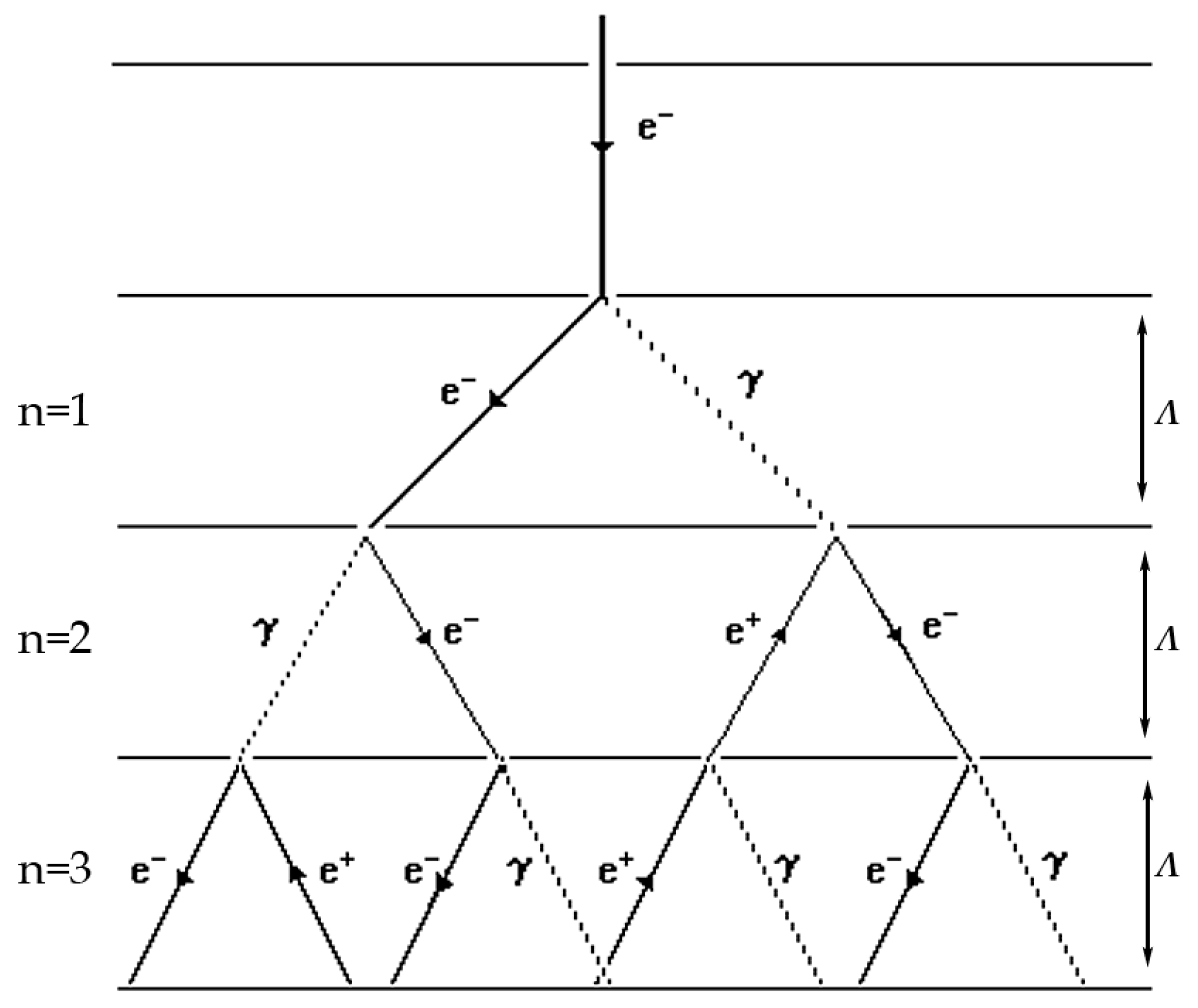
- Attenuation length, or radiation length: denoted by a capital “Λ” (or X0) (cm), is defined as the length needed to reduce the energy of a particle to a value 1/e of its original (0.3678, so of 36.78%).
- Interaction depth or radiation depth: denoted by a capital “X”, is the path traveled by a particle in a medium and is measured in gcm−2 (length times the density of the medium: cm∙g∙cm−3 = g∙cm−2, from which it can be seen that λ = X/ρ, thus g∙cm−2/g∙cm−3 = cm). Sometimes these quantities may confound because among scientists there is no uniform denotation; some authors express both “λ” and “Λ” multiplied by the density of the medium (in that case λ and Λ are usually denoted, respectively, by λ’ and Λ’, or by other symbols), becoming likewise gcm−2. Even worse, some authors use the lowercase or uppercase Greek letter lambda indifferently.
- Meter of water equivalent (mwe): it is a unit of measurement for attenuation that expresses the thickness of any material as a function of its density in relation to the thickness of a meter of water. This unit is equivalent to the length (thickness) of a medium in meters times its density: mwe = L (medium) [m] ρ [gcm−3]. For instance, 0.127 m of iron is equivalent to an mwe (in other words, a meter of water has the same effect as 12.7 cm of iron). The mwe is sometimes convenient, as it makes it possible to directly and intuitively compare the thickness of matter that cosmic rays have to pass through, like in underground laboratories. For example, given that “standard” rock has a density of 2.65 gcm−3, a detector placed 380 m below the ground has an attenuation of 1000 mwe, or equal to a column of water measuring one kilometer.
2.1. Photon Intensity Reduction in Matter
2.2. Probability of Interaction
2.3. Development of Electromagnetic Showers in Matter
- The decay of neutral pions results in the emission of two gamma rays with a combined energy of at least 140 MeV;
- Electrons from muon decay and other accelerated electrons have a 30–40% chance of producing bremsstrahlung;
- The annihilations between electrons and positrons produce a characteristic energy line at 0.51 MeV;
- Nuclear collisions yield neutrons with energies of approximately 10 MeV; these neutrons can undergo scattering or be captured by nitrogen-14 and oxygen-16, resulting in the creation of excited states that emit characteristic gamma energies;
- Gamma rays below 2 MeV degrade slowly by multiple Compton scattering;
- Photons around 30 keV have interactions through the photoelectric effect.
3. Experimental Setup
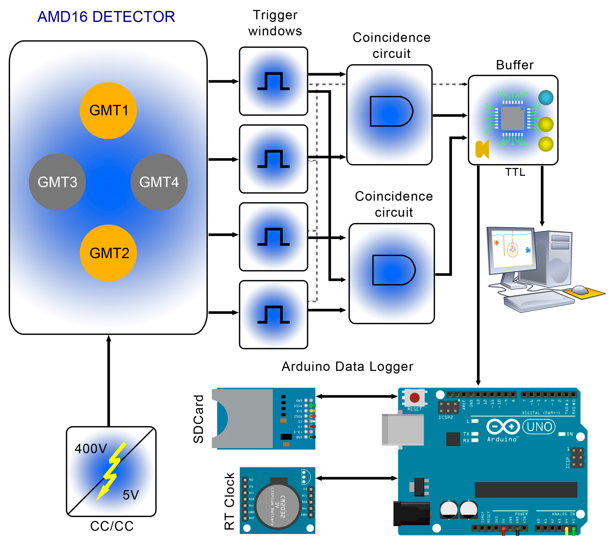
3.1. The Cosmic Ray Telescope and Shower Detector AMD16
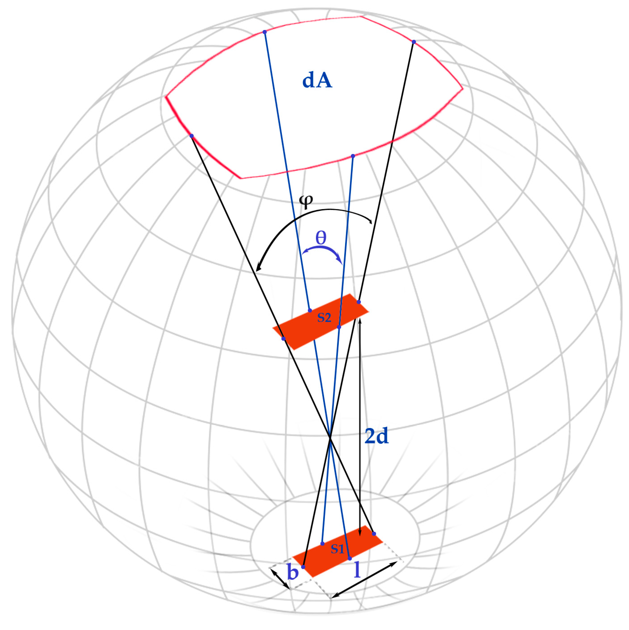
3.2. Geometry of the Muon Telescope and Shower Detector
3.3. Methodology for Detecting and Measuring Particle Showers in Water
4. Results and Analysis
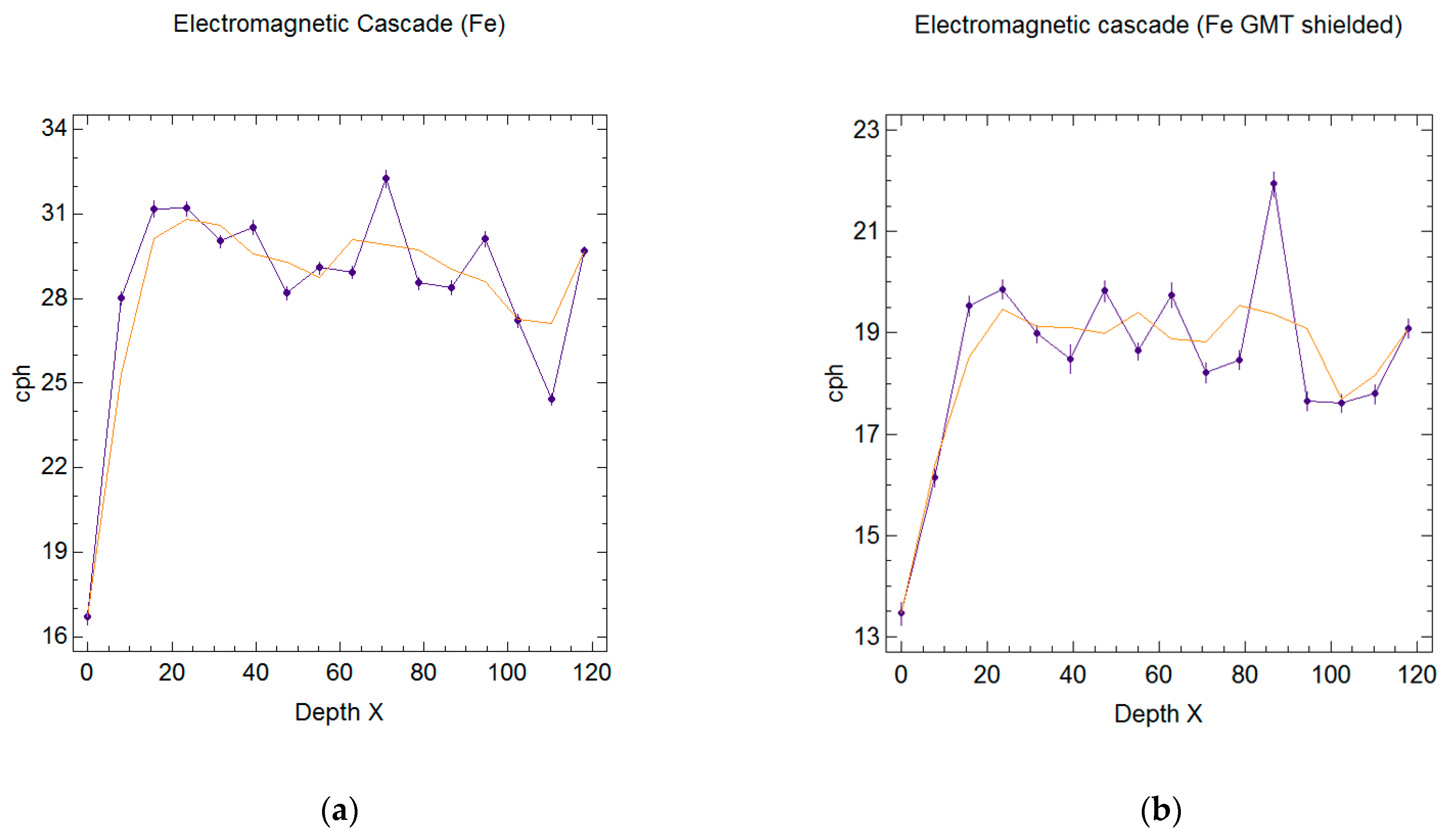
4.1. Electromagnetic Cascades in Iron
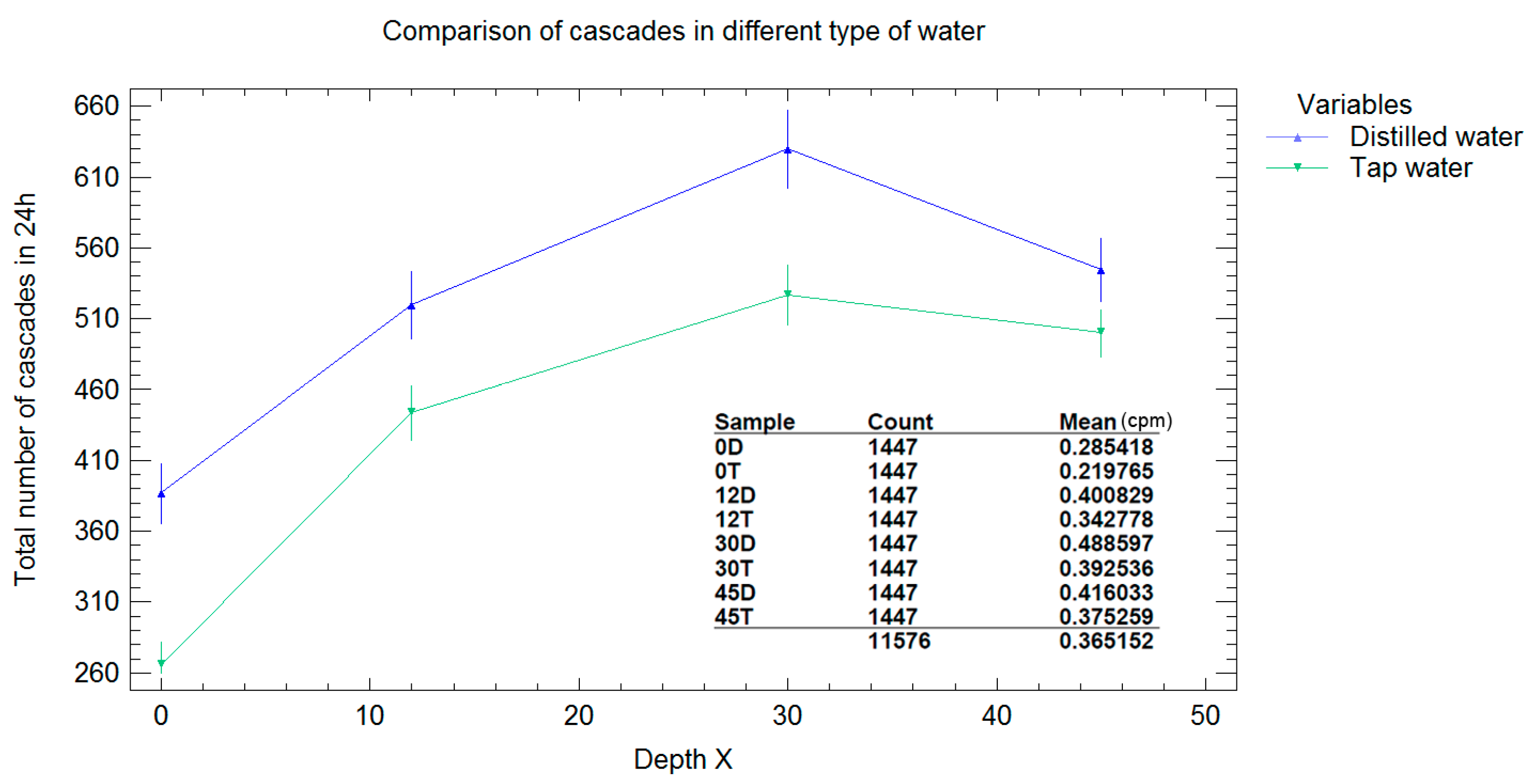
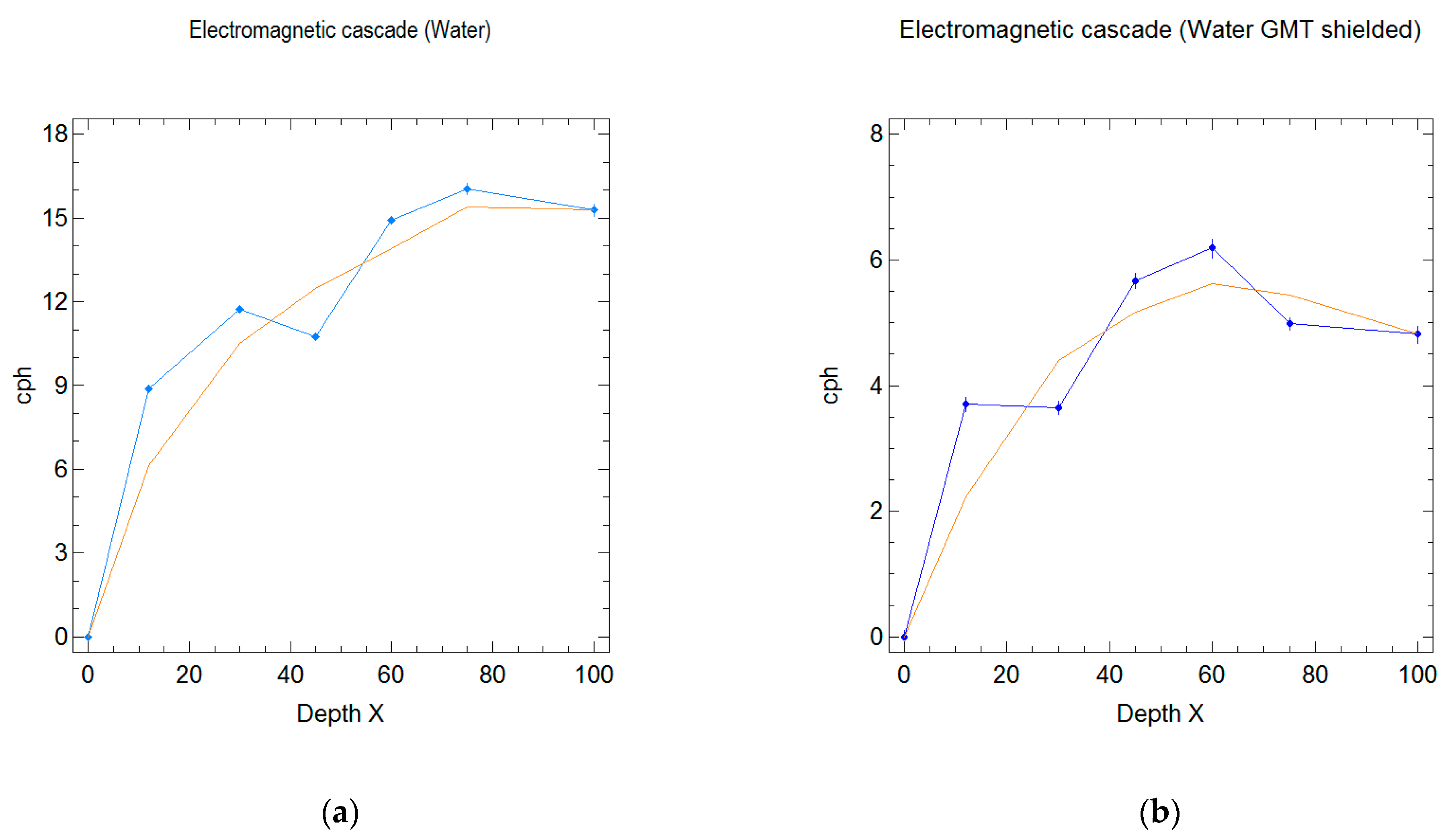
4.2. Electromagnetic Cascades in Water
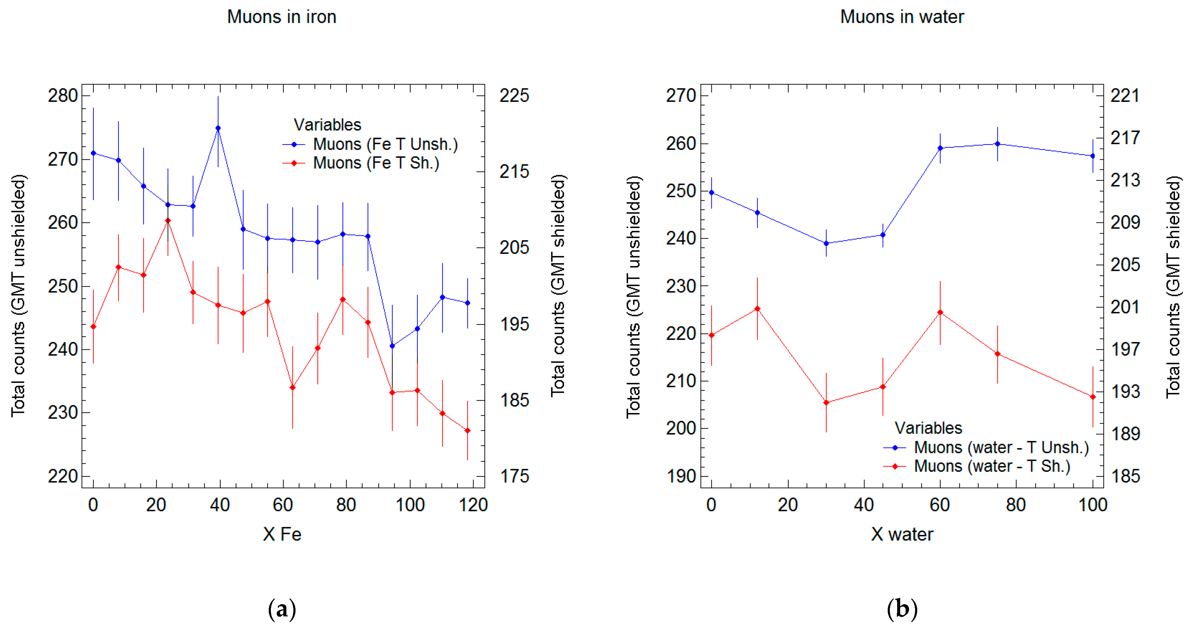
4.3. Muon Absorption in Water and Iron
5. Discussion
- The simpler explanation is that muons belonging to the same atmospheric shower pass through the water and simultaneously hit all the GMTs. It would be extremely difficult to avoid this possibility, even with a more complex instrument setup and anti-coincidence circuits;
- Another possible explanation is that sometimes an energetic muon can produce a shower directly inside the instrument by scattering tertiary particles from the metallic surface of the sensors, leading to the counting of a shower event;
- The phenomenon could result from a combination of the above factors, and local natural radioactivity.
Author Contributions
Funding
Data Availability Statement
Acknowledgments
Conflicts of Interest
References
- Bonolis, L. Walther Bothe and Bruno Rossi: The birth and development of coincidence methods in cosmic-ray physics. Am. J. Phys. 2011, 79, 1133–1150. [Google Scholar] [CrossRef]
- Rossi, B. Cosmic Rays; McGraw-Hill: New York, NY, USA, 1964; pp. 48–89. [Google Scholar]
- Rossi, B. Nachweis einer Sekundärstrahlung der durchdringenden Korpuskularstrahlung. Phys. Z. 1932, 33, 304–305. [Google Scholar]
- Lechner, A. Particle Interactions with Matter. CERN Yellow Rep. Sch. Proc. 2018, 5, 47. [Google Scholar] [CrossRef]
- Grieder, P.K.F. (Ed.) Cosmic Ray Properties, Relations and Definitions. In Cosmic Rays at Earth; Elsevier: Amsterdam, The Netherlands, 2001; Chapter 1; pp. 1–53. ISBN 9780444507105. [Google Scholar] [CrossRef]
- Grieder, P.K.F. (Ed.) Cosmic Rays in the Atmosphere. In Cosmic Rays at Earth; Elsevier: Amsterdam, The Netherlands, 2001; Chapter 2; pp. 55–303. ISBN 9780444507105. [Google Scholar] [CrossRef]
- Grieder, P.K.F. (Ed.) Cosmic Rays at Sea Level. In Cosmic Rays at Earth; Elsevier: Amsterdam, The Netherlands, 2001; Chapter 3; pp. 305–457. ISBN 9780444507105. [Google Scholar] [CrossRef]
- Matthews, J. A Heitler model of extensive air showers. Astropart. Phys. 2005, 22, 387–397. [Google Scholar] [CrossRef]
- Oxford Physics. Passage of Particles Through Matter. Available online: https://www2.physics.ox.ac.uk/sites/default/files/Passage.pdf (accessed on 23 June 2023).
- Arcani, M.; Conte, E.; Monte, O.D.; Frassati, A.; Grana, A.; Guaita, C.; Liguori, D.; Nemolato, A.R.M.; Pigato, D.; Rubino, E. The Astroparticle Detectors Array—An Educational Project in Cosmic Ray Physics. Symmetry 2023, 15, 294. [Google Scholar] [CrossRef]
- De Angelis, A. Domenico Pacini, uncredited pioneer of the discovery of cosmic rays. Riv. Nuovo Cim. 2010, 33, 713–756. [Google Scholar] [CrossRef]
- Maghrabi, A.; Makhmutov, V.S.; Almutairi, M.; Aldosari, A.; Altilasi, M.; Philippov, M.V.; Kalinin, E.V. Cosmic ray observations by CARPET detector installed in central Saudi Arabia-preliminary results. J. Atmos. Sol. Terr. Phys. 2020, 200, 105194. [Google Scholar] [CrossRef]
- Rajpoot, H.C. HCR’s Theory of Polygon (proposed by harish chandra rajpoot) solid angle subtended by any polygonal plane at any point in the space. Int. J. Math. Phys. Sci. Res. 2014, 2, 28–56. [Google Scholar]
- Centronic, Geiger Müller Tubes. Available online: https://www.rsp-italy.it/Electronics/Databooks/Centronic/_contents/Centronic%20-%20Geiger%20Tube%20Theory%20-%20ISS1.pdf (accessed on 23 June 2023).
- Korff, S.A. Electron and Nuclear Counters Theory and Use; D. Van Nostrand Company, INC.: Berlin, Germany, 1946; p. 145. [Google Scholar]
- George, E.P.; Jánossy, L.; McCaig, M.; Stuart, B.P.M. The ‘second maximum’ of the shower transition curve of cosmic radiation. Proc. R. Soc. Lon. Ser. A Math. Phys. Sci. 1942, 180, 219–224. [Google Scholar] [CrossRef]
- Kobayashi, K.; Ise, J.-I.; Aoki, R.; Kinoshita, M.; Naito, K.; Udo, T.; Kunwar, B.; Takahashi, J.-I.; Shibata, H.; Mita, H.; et al. Formation of Amino Acids and Carboxylic Acids in Weakly Reducing Planetary Atmospheres by Solar Energetic Particles from the Young Sun. Life 2023, 13, 1103. [Google Scholar] [CrossRef] [PubMed]
- Globus, N.; Blandford, R.D. The Chiral Puzzle of Life. Astrophys. J. Lett. 2020, 895, L11. [Google Scholar] [CrossRef]
- Todd, P. Cosmic radiation and evolution of life on earth: Roles of environment, adaptation and selection. Adv. Space Res. 1994, 14, 305–313. [Google Scholar] [CrossRef]


| Material | Density (gcm−3) | Λ (cm) | Ec (MeV) |
|---|---|---|---|
| Al | 2.7 | 8.9 | 42.7 |
| Fe | 7.87 | 1.76 | 21.7 |
| Pb | 11.4 | 0.56 | 7.4 |
| H2O | 1 | 36 | 93 |
| Air | 10−3 1 | 3.7∙104 1 | ≅100 1 |
| Water X (gcm−2) | Mean (cpm) | Stnd. Error | Lower Limit | Upper Limit | ||||
|---|---|---|---|---|---|---|---|---|
| (1) | (2) | (1) | (2) | (1) | (2) | (1) | (2) | |
| 0 | 0.20 | 0.22 | 0.012 | 0.016 | 0.17 | 0.19 | 0.22 | 0.25 |
| 12 | 0.35 | 0.28 | 0.015 | 0.015 | 0.32 | 0.25 | 0.38 | 0.31 |
| 30 | 0.40 | 0.28 | 0.016 | 0.014 | 0.36 | 0.25 | 0.43 | 0.31 |
| 45 | 0.38 | 0.31 | 0.013 | 0.016 | 0.35 | 0.28 | 0.40 | 0.35 |
| 60 | 0.45 | 0.32 | 0.018 | 0.020 | 0.41 | 0.28 | 0.48 | 0.36 |
| 75 | 0.47 | 0.30 | 0.030 | 0.014 | 0.41 | 0.27 | 0.53 | 0.33 |
| 100 | 0.45 | 0.30 | 0.030 | 0.018 | 0.39 | 0.27 | 0.51 | 0.34 |
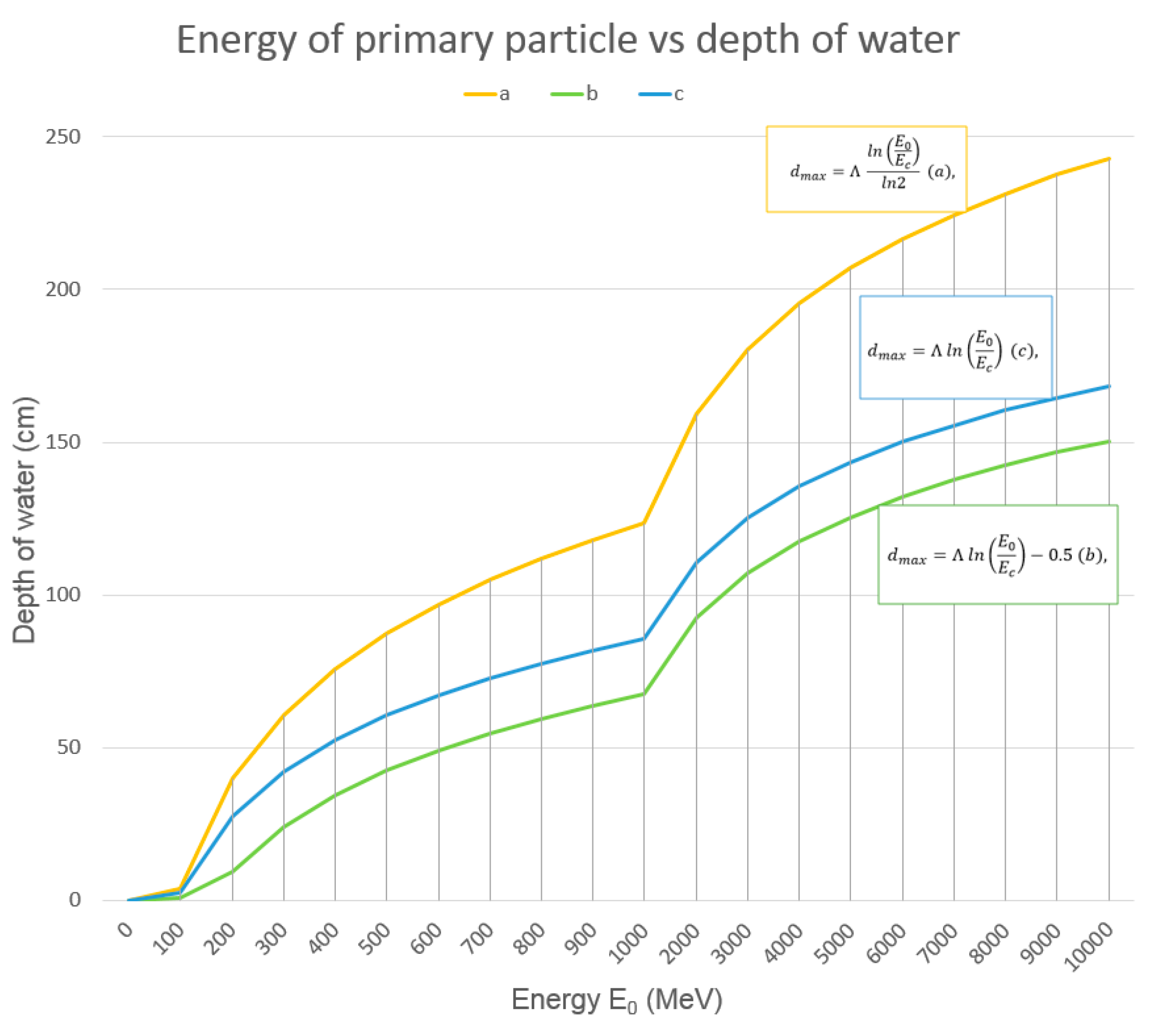
| Element | E0 (Equation (16a)) (MeV) | E0 (Equation (16b)) (MeV) | E0 (Equation (16c)) (MeV) |
|---|---|---|---|
| Pb | 60 | 200 | 150 |
| Fe | 80 | 200 | 150 |
| H2O * | 300 | 900 | 500 |
| 400 | 1000 | 750 |
| Experiment | Intercept | Slope | R2 (%) | Std. Err. of Estimate | Mean Abs. Err. | Model |
|---|---|---|---|---|---|---|
| Iron GMTs unshielded | 5.6 | −0.00087 | 75 | 0.020 | 0.013 | e(5.6−0.00087×Fe) |
| Iron GMTs shielded | 5.3 | −0.00084 | 64 | 0.025 | 0.017 | e(5.3−0.00084×Fe) |
Disclaimer/Publisher’s Note: The statements, opinions and data contained in all publications are solely those of the individual author(s) and contributor(s) and not of MDPI and/or the editor(s). MDPI and/or the editor(s) disclaim responsibility for any injury to people or property resulting from any ideas, methods, instructions or products referred to in the content. |
© 2023 by the authors. Licensee MDPI, Basel, Switzerland. This article is an open access article distributed under the terms and conditions of the Creative Commons Attribution (CC BY) license (https://creativecommons.org/licenses/by/4.0/).
Share and Cite
Arcani, M.; Liguori, D.; Grana, A. Exploring the Interaction of Cosmic Rays with Water by Using an Old-Style Detector and Rossi’s Method. Particles 2023, 6, 801-818. https://doi.org/10.3390/particles6030051
Arcani M, Liguori D, Grana A. Exploring the Interaction of Cosmic Rays with Water by Using an Old-Style Detector and Rossi’s Method. Particles. 2023; 6(3):801-818. https://doi.org/10.3390/particles6030051
Chicago/Turabian StyleArcani, Marco, Domenico Liguori, and Andrea Grana. 2023. "Exploring the Interaction of Cosmic Rays with Water by Using an Old-Style Detector and Rossi’s Method" Particles 6, no. 3: 801-818. https://doi.org/10.3390/particles6030051
APA StyleArcani, M., Liguori, D., & Grana, A. (2023). Exploring the Interaction of Cosmic Rays with Water by Using an Old-Style Detector and Rossi’s Method. Particles, 6(3), 801-818. https://doi.org/10.3390/particles6030051