Article

A Machine-Learning-Based Method to Detect Degradation of Motor Control Stability with Implications to Diagnosis of Presymptomatic Parkinson’s Disease: A Simulation Study

by
Vrutangkumar V. Shah
1,2,
Shail Jadav
2,
Sachin Goyal
2,3,4,* and
Harish J. Palanthandalam-Madapusi
4
1
Balance Disorder Laboratory, Department of Neurology, Oregon Heath and Science University, Portland, OR 97239, USA
2
SysIDEA Robotics Lab, Mechanical Engineering, Indian Institute of Technology (IIT), Gandhinagar 382055, Gujarat, India
3
Department of Mechanical Engineering, University of California, Merced, CA 95343, USA
4
Health Science Research Institute, University of California, Merced, CA 95343, USA
*
Author to whom correspondence should be addressed.
Appl. Sci. 2023, 13(17), 9502; https://doi.org/10.3390/app13179502
Submission received: 4 March 2023 / Revised: 1 April 2023 / Accepted: 19 April 2023 / Published: 22 August 2023
(This article belongs to the Section Biomedical Engineering)

Abstract

:
Background and aim: Parkinson’s disease (PD), a neuro-degenerative disorder, is often detected by the onset of its motor symptoms such as rest tremor. Unfortunately, motor symptoms appear only when approximately 40–60% of the dopaminergic neurons in the substantia nigra are lost. In most cases, by the time PD is clinically diagnosed, the disease may already have started 4 to 6 years beforehand. There is therefore a need for developing a test for detecting PD before the onset of motor symptoms. This phase of PD is referred to as Presymptomatic PD (PPD). The motor symptoms of Parkinson’s Disease are manifestations of instability in the sensorimotor system that develops gradually due to the neurodegenerative process. In this paper, based on the above insight, we propose a new method that can potentially be used to detect the degradation of motor control stability, which can be employed for the detection of PPD. Methods: The proposed method tracks the tendency of a feedback control system to transition to an unstable state and uses a machine learning algorithm for its robust detection. This method is explored using a simple simulation example consisting of a simple pendulum with a proportional-integral-derivative (PID) controller as a conceptual representation for both healthy and PPD individuals with a noise variance of 0.01 and a noise variance of 0.1. The present study adopts a longitudinal design to evaluate the effectiveness of the proposed methodology. Specifically, the performance of the proposed approach, with specific choices of features, is compared to that of the Support Vector Machine (SVM) algorithm for machine learning under conditions of incremental delay-induced instability. This comparison is made with results obtained using the Longitudinal Support Vector Machine (LSVM) algorithm for machine learning, which is better suited for longitudinal studies. Results: The results of SVM with one choice of features are comparable with the results of LSVM for a noise variance of 0.01. These results are almost unaffected by a noise variance of 0.1. All of the methods showed a high sensitivity above 96% and specificity above 98% on a training data set. In addition, they perform very well with the validation synthetic data set with sensitivity above 95% and specificity above 98%. These results are robust to further increases in noise variance representing the large variances expected in patient populations. Conclusions: The proposed method is evaluated on a synthetic data set, and the machine learning results show a promise and potential for use for detecting PPD through an early diagnostic device. In addition, an example task with physiological measurement that can potentially be used as a clinical movement control test along with representative data from both healthy individuals and PD patients is also presented, demonstrating the feasibility of performing a longitudinal study to validate and test the robustness of the proposed method.

1. Introduction

Parkinson’s disease (PD) is the second largest progressive neurodegenerative disorder of the central nervous system [1]. It is characterized by several motor symptoms such as tremor at rest, rigidity, bradykinesia, and postural instability. Generally, the clinical diagnosis is based on a combination of clinical symptoms, a thorough history of patients, and a response to levodopa [1,2,3]. It is reported that motor symptoms appear only when approximately 40–60% of the dopaminergic neurons in the substantia nigra are lost [4,5,6,7]. In most cases, by the time PD is diagnosed, the disease may have already started 4 to 6 years beforehand [7]. There is therefore is a need to develop a test for detecting PD before the onset of the motor symptoms (called Presymptomatic PD (PPD) [8,9]). Such a test would help a clinician not only in detecting PPD, but also in monitoring the progression of PD or in monitoring efficacy of early therapeutic interventions [10,11]. Detecting PPD helps patients to start their treatment in the presymptomatic phase. The utilization of machine learning techniques for the early diagnosis of Parkinson’s disease is an active area of research. These efforts aim to leverage the power of these techniques to enhance the accuracy and timeliness of diagnosis [12,13,14,15,16]. It has been established that there are advantages of early pharmacological and therapeutic intervention in PD such as monoamine oxidase B inhibitors [17], catechol-o-methyl-transferase inhibitors [18], amantadine [19], amplitude training [20], reciprocal pattern training [21], and gait-balance training [22], including a reduction in symptoms, particularly dyskinesia, and the delay of levodopa initiation [23]. Both the reduction in symptoms and the potential for slowing disease progression can have a significant impact on improving patients’ quality of life [23].
Although there have been recent advances in identifying potential biomarkers [24], including genetic [25,26] and neuroimaging techniques [11] that help in detecting PD, these are still in the early stages, and further work is needed in this direction. Further, it has also been recognized that a variety of nonmotor symptoms associated with PD may be observed years before the onset of motor symptoms and hence may be used as markers for detecting PPD [27]. Examples of these nonmotor symptoms are olfactory loss [28,29], rapid eye movement sleep behavior disorders [30,31,32], bowel dysfunction, and so on [27,33,34]. Recently, reference [7] proposed that a combination of tests (including smell test, transcranial sonography, and SPECT) could be helpful in detecting PPD. Further, Ref [35] proposed a general methodology and an automatic system that can be used for the detection of presymptomatic phase or diagnosis, and/or to monitor the treatment effectiveness for a variety of neurological disorders based on eye movement data for various stimuli. An important ingredient that is lacking in these methodologies is that they are empirical and are not based primarily on an understanding of the mechanism causing these symptoms.
As widely noted in the literature [36,37,38,39,40,41,42,43,44,45,46,47,48,49], the sensorimotor system of a healthy individual may be seen as a stable control system, while the sensorimotor system of an individual with PD showing motor symptoms may be viewed as a control system with instabilities. The source and mechanism of these instabilities remain topics of debate and investigation with delay-induced instability (with higher loop-delay in PD causing the instability, further explained in Section 2.1) being one of the prominent theories [42,46,47,49]. In general, the latencies in the sensorimotor loop are also known to be amplified and cause instabilities in other conditions as well, such as Multiple Sclerosis (MS) and stroke survivors [50].
In this paper, we propose a method for detecting this degradation in stability, which can then be applied to detecting PPD based on observing the progression of the tendency of the sensorimotor loop to develop instabilities before the instability manifests itself as symptoms. Here, we do not concern ourselves with the source or mechanism of the instability and develop a method that could be utilized for any instability in general. This proposed method is further fleshed out through a numerical study. We employ a simple pendulum with a PID controller as a conceptual representation of the sensorimotor loop to simulate motor control tasks in healthy and PPD individuals for this analysis. We also present representative human subject data collected through such an example clinical test, thereby demonstrating the feasibility of the proposed method.
The main contribution of this study is to propose a method to track the tendency of a feedback control system to transition to an unstable state and using machine learning algorithms for its robust detection. Specifically, we employ a simple simulation example consisting of a simple pendulum with a PID controller as a conceptual representation for both healthy and PPD individuals with a noise variance of 0.01 and a noise variance of 0.1. To show the efficacy of the proposed method, we compare our results of the SVM algorithm for machine learning with two sets of proposed features, C1 and C2, with the results of the LSVM algorithm for machine learning. The results of SVM with feature C2 are comparable with the results of LSVM for a noise variance of 0.01. These results are almost unaffected by a noise variance of 0.1. All of the methods showed a high sensitivity of above 96% and specificity of above 98% on a training data set. In addition, they perform very well with the synthetic validation data set with a sensitivity above 95% and specificity above 98%. Thus, our proposed method is evaluated on a synthetic data set, and the machine learning results show promise and potential for use in detecting PPD through an early diagnostic device. In addition, we have shown the feasibility of the proposed method to estimate a pole from a clinical test that may be used as a regular health checkup to track the progression of the poles and hence the probability of developing Parkinson’s disease in near future.
The conceptual framework of the proposed method is described in detail in Section 2.2, the simulation example used for our numerical study in Section 2.3, and potential methods to classify whether particular data are from healthy individuals or an individual with PPD in Section 2.3.1 and Section 2.3.2. The results of the numerical study are described in Section 3. An example task and associated data collected from human subjects are presented in Section 3.2. The longitudinal study needed to validate the method will be taken up as future work. Finally, we discuss further steps needed to validate the proposed method in Section 4 and close with the conclusion in Section 5.

2. Methods

In this section, we first describe a simple representation of the sensorimotor loop. Subsequently, we describe how we leverage the insight that in PD, the instability in the sensorimotor loop develops gradually over a period of time, to propose an approach to detecting PPD. Based on the proposed approach, we perform numerical simluations using a simplified representation of a sensory–motor loop to generate synthetic data and test the method using a numerical study.

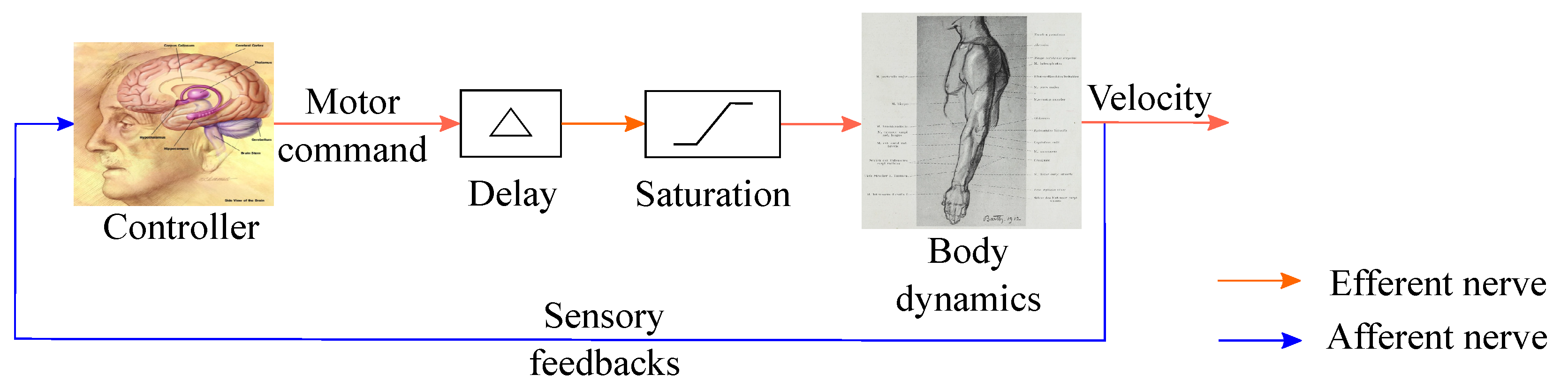
2.1. Sensorimotor Loop Representation

One can represent the motor control (movement control) in humans as a simple feedback control system of the form shown in Figure 1. In the schematic shown, the body dynamics is the natural dynamics in the absence of any neural control of the body part of interest (e.g., hand). The feedback path represents all sensory feedback, including proprioceptive feedback, visual feedback, and tactile feedback. These types of sensory feedback are carried to the controller (brain) by afferent nerves. The controller represents the neurosystem’s logic, which continuously compares the kinematic variables from sensory feedback (e.g., actual velocity) with the desired kinematic variables (e.g., desired velocity) to determine the motor command. This motor command is then conveyed through the efferent nerves and results in muscle actions to obtain the desired response. We refer to this closed-loop feedback system consisting of motor actions and sensory feedback as the human sensorimotor system. As there are various time delays in the human sensorimotor system, including delays due to nerve conduction times and information processing time, for simplicity, we lump all sensorimotor system delays (delays in various portions of the sensorimotor system) into one transport delay in the closed-loop feedback system. Finally, the saturation in the loop approximates the physiological limit of the transmission of neural control actions [51].
A number of studies [36,37,38,42,45,47,48,49,52] have observed that increased sensorimotor loop delay in PD tends to destablize the sensorimotor system. This is supported by the observation that response time in patients with PD is larger than that in healthy individuals [53,54,55,56]. According to these observations, the sensorimotor system of a healthy individual is a control system with a smaller delay, and the sensorimotor system of an individual with PD is a control system with a larger delay. Thus, this larger delay, that is, a delay beyond a certain threshold, leads to instability in the human sensorimotor system. This observation also explains some of the clinical features of Parkinsonian rest tremors [47,49] and provides a possible explanation of how high-frequency deep brain stimulation suppresses low-frequency rest tremors [57]. There are some works that also consider other possibilities for the source of instabilities including an increased gain in the sensorimotor loop [42]. However, as stated earlier, the subsequent development will not rely on this assumption but simply focus on the degradation of stability and will be applicable regardless of the source of instability.
With this background, in Section 2.2, we provide the main concept of the proposed methodology.

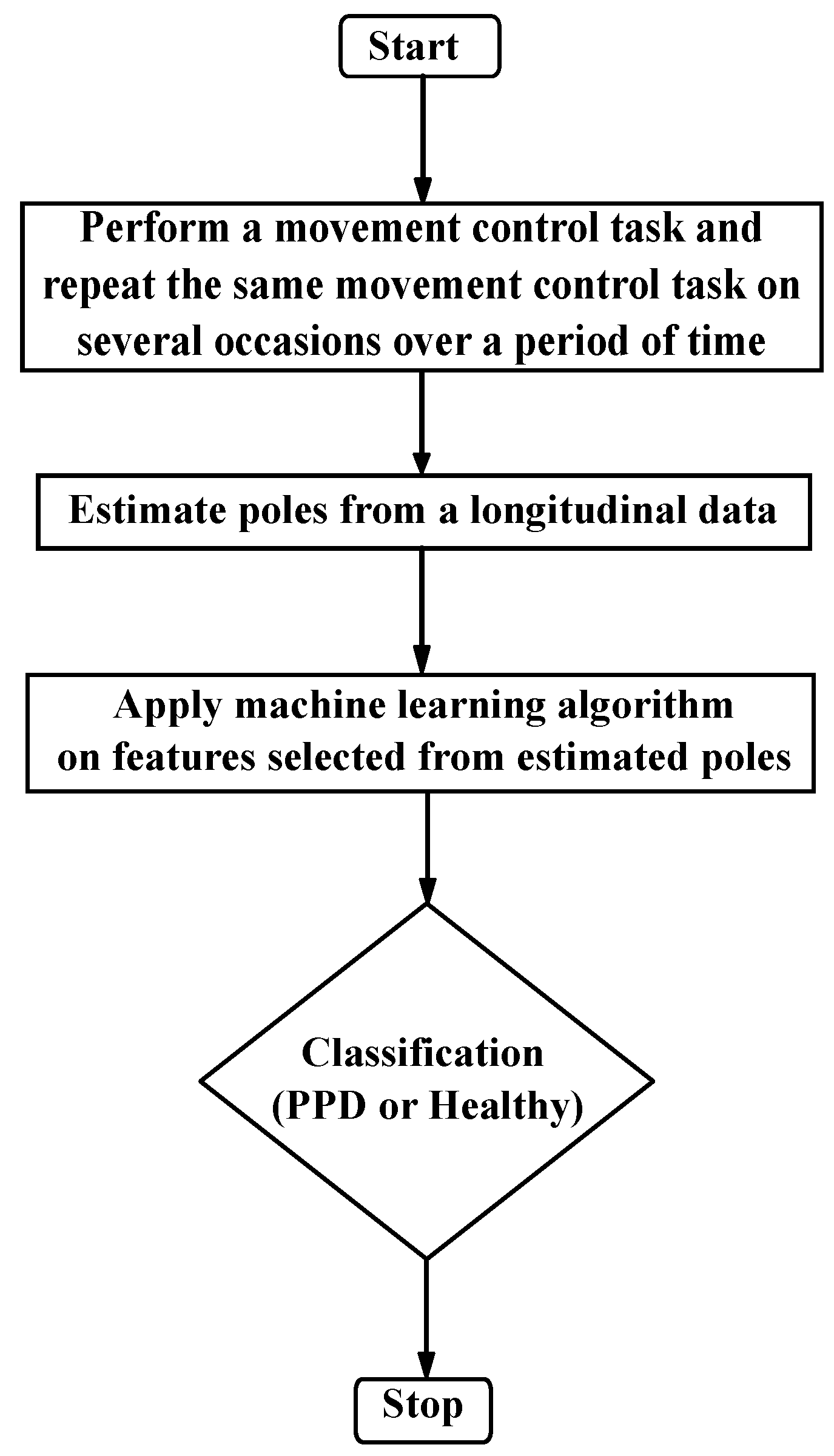
2.2. Proposed Approach for Detecting Presymptomatic Parkinson’s Disease (PPD)

Based on the insight of degrading stability in the sensorimotor loop, the proposed approach hinges on the detection of the transition of the human sensorimotor system from a stable system (healthy individual) to an unstable system (individual with PD) on the basis of a response recorded from a simple movement control task in the clinic and repeated several times over a period of time. Note that we expect this transition of the human sensorimotor system from a stable to an unstable system to be gradual, as PD is a slowly progressing disease.
In control system theory, the poles of a linearized system are a set of complex numbers that represent the nature of (and more specifically the exponents associated with) the transient behavior and thus the stability of that system. The poles of the dynamical system are also roots of differential equations that govern the system’s dynamics. A system with poles in the left-half of the complex plane is stable, that is, transient response decays with time, whereas a system with at least one pole in the right half of the complex plane is unstable, that is, the transient response grows with time. We therefore propose to use the poles as a measure of stability of the representative human sensorimotor system involved in a specified clinical task.
The proposed approach can be summarised as follows. A subject performs a series of specific clinical tasks on several occasions repeated over a period of time (not necessarily at equal intervals), and poles are estimated from these data using an algorithm (explained in Section 2.3.1). Finally, a classification algorithm is applied to the estimated poles to classify whether a particular individual is healthy or has PPD.
The degradation of stability refers to the gradual movement of at least one pole towards the right half of the complex plane. Thus, monitoring the movement of the pole(s) over time is necessary to observe this phenomenon, rather than evaluating them at a single time instant. Consequently, participants must undergo repetitive clinical movement control tests on multiple occasions over a period of time, such as during routine yearly checkups. The detection of significant movement of at least one estimated pole towards the right half of the complex plane during these clinical tasks indicates the possibility of PPD. The transition of the pole(s) towards the right-half of the complex plane occurs gradually, thereby requiring the application of repetitive clinical movement control tests for several years to track the movement of the pole(s) and facilitate the identification of the disease. Therefore, the validation of our proposed approach using real subjects would necessitate a large-scale study over a prolonged period.
We now consider a simple simulation example to further detail the proposed method.

2.3. Simulation Example

For our numerical exploration, we use a simulation example. As shown in Figure 1, we use a simple pendulum to represent the dynamics of the task and a Proportional Integral Derivative (PID) as a controller, along with a delay and saturation in a unity feedback configuration. The simple pendulum has length L, mass M, and a damping coefficient C. For our simulation, we use L = 0.65 m, M = 3.5 Kg, C = 3.375 Kgm/s, and a PID controller with the proportional gain k p = 15 , integral gain k i = 4 Hz, and derivative gain k d = 0.5 s. All simulations were carried out using MATLAB & Simulink of MathWorks (Natick, MA, USA).
This simulation example is similar to a movement control task in a clinic and has the same structure as shown in Figure 1, which is similar to other examples in the literature [36,42,47,49,57]. To simulate the degradation of stability, we first consider a small and constant delay as a representation of the human sensorimotor system of a healthy individual, and a gradually increasing delay as a representation of the human sensorimotor system of an individual with PPD. Note that this gradual increase in the delay is still below the delay threshold; that is, the delay has increased but not to the extent that it destabilizes the human sensorimotor system leading to visible motor control symptoms. Similar to delay analysis, to demonstrate that the method works equally well for other mechanisms of instability, we subsequently also consider a constant gain as a representation of the human sensorimotor system of a healthy individual and a gradual increment in gain as a representation of the human sensorimotor system for an individual with PPD. Analogous to delay, the gain is increased but not to the extent that it destabilizes the human sensorimotor system.
Procedure for generating a synthetic data set: As explained in Section 2.2, a subject needs to repeat the same clinical task on several occasions over a period of time. To mimic within-subject variability in the sensorimotor delay (or gain) values over a period of time due to various physiological factors, we consider additional stochasticity around the constant value of the delay (or gain) representing healthy individuals and a gradual increasing delay (or gain) value representing PPD individuals. This stochasticity is assumed to follow a Gaussian distribution. Further, to represent noise in the human sensorimotor system, we introduce system and measurement noise with zero mean and Gaussian distribution. Next, we use these sensorimotor delay (or gain) values in the simulation example to generate simulated responses (similar to data from a clinical task) and generate several instances of the same task repeated over a period of time. As an example, Figure 2 shows the simulated data of a single clinical task. Following this procedure, we generate a synthetic data set simulating 500 instances of a sensorimotor loop system with a constant gain and delay for healthy individuals and 500 instances of sensorimotor loop system with a gradual increment in gain and delay representing PPD. These synthetic data represent the 1000 individuals for training and validation needed for the machine learning algorithm. We used 600 individuals (synthetic data set) for training (60%) and 400 individuals (40%) to validate the machine learning algorithm. The numerical values of delays and gains for the generated synthetic data set are given in Appendix A.1. The training data set was used to train the model, and the validation data set was used to test the performance of the trained model.

2.3.1. Estimation of Poles from Data

To estimate the poles from the data, we propose using the Matrix Pencil Method (MPM) [58]. MPM approximates time series data by M complex exponentials. These estimated complex exponents represent the poles of the system of interest (in our case, the human sensorimotor system). The observed signal is represented as
y ( t ) i = 1 M R i e S i t + n ( t ) .
Here, y ( t ) is the simulated response, S i values are the estimates of poles, R i values are coefficients, and n ( k ) is the noise in the simulated data. A brief overview of an algorithm for estimating poles from data is given in Appendix A.2.
Figure 3 shows the real part of poles for simulated healthy and PPD individuals over a period of time, estimated from a few individuals in the synthetic data generated as described earlier. Further, it is to be noted that the synthetic data set consists of both individuals maintaining a regular frequency of visits and individuals maintaining an irregular frequency of visits; that is, the clinical tasks are not necessarily repeated at regular intervals but could be at irregular intervals.

2.3.2. Machine Learning Algorithm for Classification

Once we estimate poles from the measured data, the next step is to apply a classification algorithm for classifying whether a particular data (for example, one of the traces in Figure 3) is from the data set representing a healthy individual or the data set representing an individual with PPD. In the healthy individual data set, despite variabilities due to numerous factors, we do not expect the estimates of poles to have a significant trend of moving towards the right half of the complex plane. On the other hand, for the data set representing individuals with PPD, we expect at least one of the estimates of poles to have a significant trend of moving towards the right half of the complex plane. Now, one way to identify this significant trend compared to healthy individuals is to use simple statistical tests or a classifier based on simple thresholds. Exploring this approach with the synthetic data, we find that a reliable classification using a threshold alone is not a robust approach. This is partly due to the significant overlap between poles of the human sensorimotor system for healthy and PPD groups in simulated data (representing inter-subject variability), and perhaps partly due to the stochastic variability as apparent in Figure 3. Therefore, we explore machine learning algorithms for a more robust classification. Typically, the input to the machine learning algorithm is a set of features derived from the data. For instance, to classify whether a particular individual has a benign or malignant tumor, the tumor size and age at diagnosis are possible features to consider [59]. Using these features, a machine learning algorithm trains a model that best describes the relationship between input (features) and output (class) for those data and uses this model to classify the new data. In the following subsections, we briefly describe two machine learning algorithms.
  • Support Vector Machine: Support Vector Machine (SVM) [60] is a supervised machine learning algorithm, that given the training data with their features and class labels identified a priori, determines the maximum margin hyperplane in feature space. Maximum margin hyperplane is a plane in feature space from which the distance to the nearest data points of both classes is maximized. Once the maximum margin hyperplane is determined, depending on the position of the new data set in the feature space, that is, whether new data are lying below the hyperplane or above the hyperplane, each new data set is classified as either Class 1 or Class 2. In the case of outliers in data or data that are not linearly separable, a variant of SVM is used that finds a non-linear boundary to separate both classes of data. For further details, refer to [60].
    Feature Selection: Feature selection is an important aspect of the success of machine learning algorithms. A good choice of features helps improve classification performance, lower computational complexity, build more generalizable models and decrease the required storage [61]. The aim of feature selection is to extract features from data that represent the characteristics of each of the classes or groups. Since we are interested in tracking the stability of the human sensorimotor system and only the real part of estimated poles in the complex plane governs the stability, we only use the real part of the estimated poles for the rest of our analysis. We explore two sets of choices (C1 and C2) for feature selection. These choices of features are then used as input to the SVM to classify whether a particular individual is healthy or has PPD.
    C1: Since we are interested in the trend of the real part of the estimated poles over a period of time, the percentage changes in the real parts of poles with respect to the baseline (the estimated poles from the simulated response of the first movement control test) and the percentage change in the successive difference in the real parts of poles between simulated responses over a period of time are the features worth considering. However, in reality, it is very likely that the clinical task is not performed at fixed intervals of time for all subjects. Hence, we consider the rate of percentage change (either per month or per year) for both of the above-mentioned quantities as features. Based on preliminary simulation results, we find that only three features are sufficient for robust classification, namely, minimum percentage change rate in the real part of the poles, maximum percentage change rate in the successive difference between tests, and real part from the first clinical movement control test.
     The calculation of the percentage change rate in the real part of the poles and percentage change rate in the successive difference between tests are given in Table 1. Here, N is the total number of clinical movement control tests that are conducted possibly at irregular time intervals. T k is the time duration between two trials, where k = 1 , 2 , , N 1 . x 1 to x N are the real parts of estimated poles, with subscripts indicating the test number.
    C2: For a second choice of features, since we are interested in determining whether the real part of estimated poles has an increasing trend, we use hypothesis testing as a tool to detect a statistically significant increasing trend in the presence of noisy data. With this approach, we use the statistical value of slope and the constant of the real part of estimated poles as features for the classification algorithm. Further, we also take the real part of the estimated poles of the simulation response of the first movement control test as the third feature as an indicator of the baseline for each individual.
  • Support Vector Machine for Longitudinal Analysis (LSVM) A recently developed method, called Longitudinal Support Vector Machine (LSVM) [62], is a method specifically developed for longitudinal data. Here, each data point takes the form of a single time series. LSVM is shown to have higher accuracy compared to SVM, linear discriminant analysis (LDA), and functional linear discriminant analysis (FLDA). Note that once we have real parts of estimated poles over a period of time, this method is formulated such that an additional feature selection is not required.

3. Results

In this section, we first test the robustness of MPM and discuss the classification results of two machine learning algorithms on the synthetic data set. First, to test the robustness of the MPM in the presence of noise, we introduce system and measurement noise with different variances. Figure 4 shows an estimate of poles for various values of delay and gains and the effect of noise with different variances on the estimation of poles, indicating that the estimates from MPM are robust to noise and disturbances. For all the data generation, we assume that system and measurement noises have the same variances.

3.1. Classification Results

Figure 5 shows a box-plot of the real part of the estimated pole for the synthetic data set containing the simulated healthy and PPD groups over a period of time. The box plot shows the median, range, and quartiles of the population distributions. It is clear from the box plot that the real part of the estimated poles remains in the same range for simulated healthy individuals and increases for PPD over a significant period of time. Next, we apply machine learning algorithms to these data.
To show the efficacy of the proposed method, we compare our results of SVM (incremental delay) with the proposed features (C1 and C2) with the results of the LSVM (incremental delay). The classification results for the simulated (incremental delay) data set with a noise variance of 0.01 are shown in Table 2 and those with a noise variance of 0.1 are shown in Table 3. It is seen from Table 2 and Table 3 that the results of SVM with features C2 are comparable with the results of LSVM. It is clear from Table 3 that the above results are almost unaffected by a noise variance of 0.1. Further, on repeating the above procedure with ten independently generated synthetic data sets, we find that the above results are reproducible. Note that all of the methods have a high sensitivity of above 96% and specificity of above 98%. In addition, they perform very well with the validation synthetic data set, with a sensitivity above 95% and specificity above 98%. All three approaches seem to perform well with this synthetic data set. With a further increase in the variance of the noise by 100%, the sensitivity and specificity only drop by a modest margin by about a dozen percentage points despite the big bump in the noise variance, and these numbers further improve if a longer duration is utilized. This is promising especially considering the much larger overlap between the healthy and PPD data in such a situation.
Next, to demonstrate that the same method is effective when the source of instability is different from an increased delay, we consider the synthetic data set with a gradual increasing gain (as mentioned in Appendix A.1). With the C1 choice of features and the SVM method, we observe that the sensitivity is 96% and the specificity is 94.33% with the training synthetic data set (incremental gain), while for the synthetic validation data set (incremental gain), the sensitivity is 98% with a specificity of 93%.

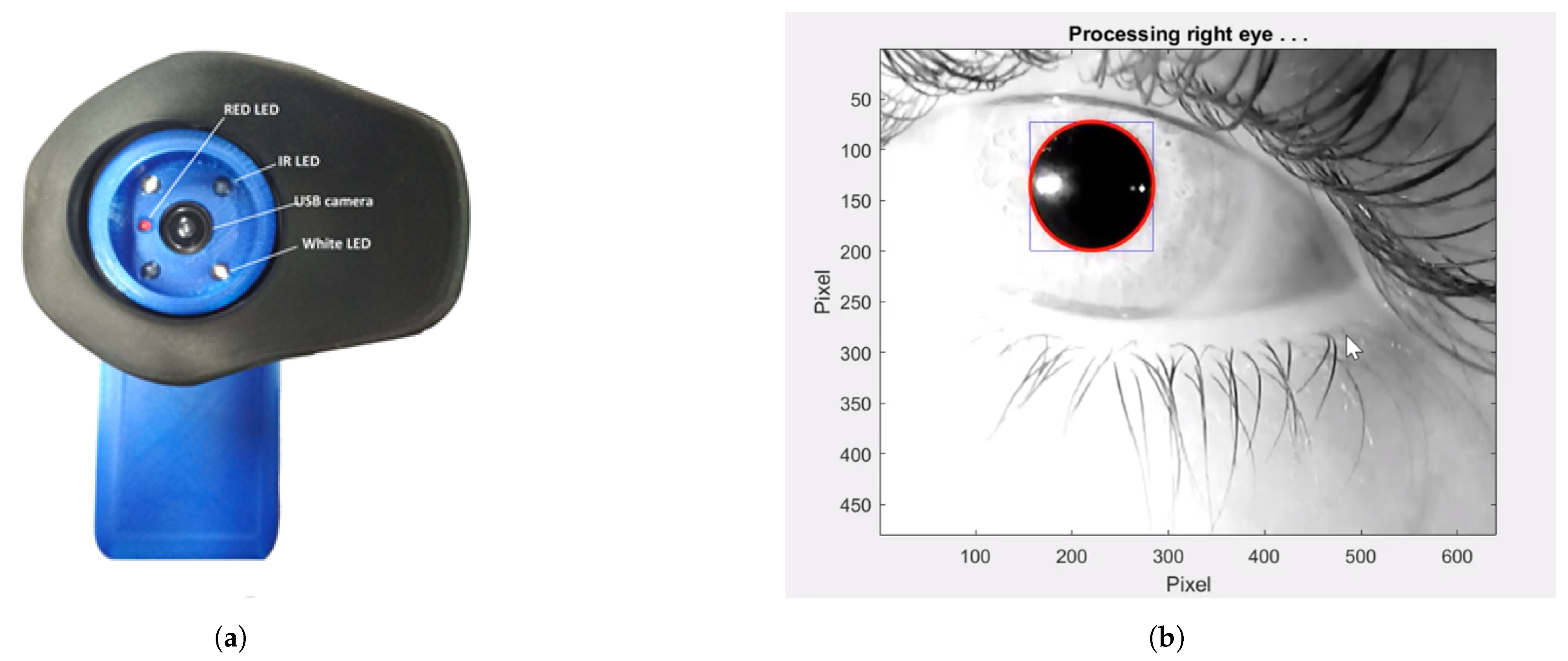
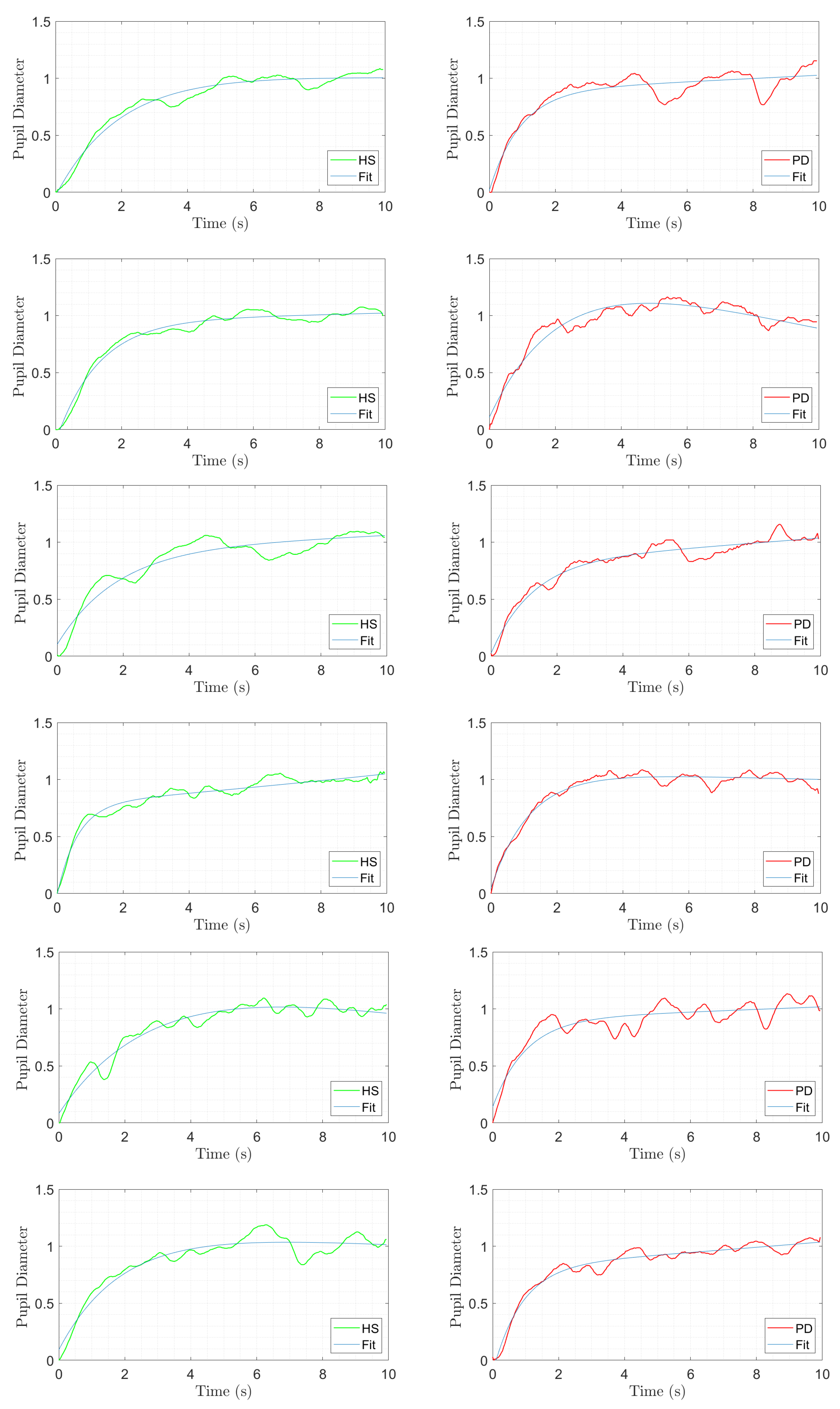
3.2. Example Task and Physiological Measurement

One of the major requirements in designing a clinical movement control test for detecting PPD is that the test should be simple and easy to execute. There are various possible clinical movement control tests, such as a spiral tracing task, in which the subject needs to trace a spiral drawn on white paper [63]; an eye tracking task, in which the subject needs to follow a circle displayed on a screen [64,65]; a compensatory tracking task, in which the subject needs to maintain the actual position of the arm with a zero reference (or initial) position of an arm displayed on the screen in the presence of an outside influence by means of compensating for the error in arm position [66]. In this work, we consider pupil dilation/constriction data to apply the proposed method. A significant latency is reported during the pupillary light reflex in patients with Parkinson’s disease [67,68], and this latency increases with the progression of the disease [69]. This latency degrades the stability of the sensory-motor loop representing the pupillary-light-reflex. Therefore, the proposed method is applicable in this situation. It is worth noting that the proposed method is equally applicable to any of the other motor control tasks mentioned above.
We developed a pupilometer in the lab, as shown in Figure 6a, that uses a camera, infrared light sources, and LEDs to stimulate the pupil (with light flashes). With this pupilometer and its onboard microcontroller, it is possible to produce different stimulation patterns of white LEDs switching on and off, and the resulting pupil response is recorded as a video. Further, using relatively straightforward image processing techniques, the pupil diameter as a function of time is estimated from the recorded video. This is a simple portable device and a comfortable task for patients and can be conducted in any clinical environment without any special arrangements. A sample screenshot of the video recorded by the device after applying image processing to detect the pupil diameter is shown in Figure 6b.
The device was utilized to gather data from both age-matched healthy control subjects and patients with Parkinson’s disease (PD). Prior to participating in the experiment, all participants provided written informed consent, and the institute’s ethics committee approved the experimental protocols. During the test, participants were instructed to focus on the red LED located at the center of the screen, with the LED light source being turned on for 10 s and then turned off for 10 s. The procedure was repeated five times within a single trial, and three sets of trials were conducted. The pupil diameter data obtained from each trial was considered a step response, and matrix pencil methods were employed to estimate poles representing the motor control dynamics.
The output of the pupil detection algorithm for a few representative PD patients (6) and age-matched healthy individuals (6) are shown in Figure 7. A total of 63 trials were conducted, and MPM was used to detect poles for all these trials; the pole data are not reported here, as the absolute values are irrelevant, and only long-term trends are relevant. The data show the feasibility of setting up a simple clinical task and the ability to generate good quality data that the MPM is able to process to generate estimates of poles. The machine-learning-based classification algorithm is, however, not applied here, as that will require long-term data from a longitudinal study. The proposed method is designed to detect long-term trends in a single patient’s data, and therefore, a comparison across patients is not of value and hence the quantitative results in Figure 6b are not discussed in detail. A longitudinal study to validate the method is planned as future work.

4. Discussion

Continuing with the approach and simulation results presented in this paper, a longitudinal study using real patient data is necessary to further investigate the effectiveness and robustness of the methods. While the proposed methodology shows potential, further testing is required to refine and develop it into a practical early-diagnosis device. The proposed methodology has potential applications in other situations, including motor performance in multiple sclerosis [70], stability of balance control [71,72], characterizing slow eye movements [73], wearable health monitoring [74], and cerebral autoregulation [75,76].
The sequence of steps required to implement the proposed approach in a clinical setting is described in Figure 8. In summary, a subject performs a series of clinical movement control tests on several occasions over a period of time (not necessarily at equal intervals) and all data are recorded. After a few clinical movement control tests spanning a significant amount of time (say several months or years), using an algorithm (explained in Section 2.3.1), poles are estimated from these data for a particular individual. Finally, a classification algorithm is applied to the estimated poles. The output of the classification algorithm classifies whether a particular individual is healthy or has PPD. This classification will directly aid clinicians in identifying individuals who are at risk of developing PD in the near future and taking necessary precautions or applying certain interventions as appropriate.
One possible clinical task with a simple pupilometer outlined in Section 3.2 can be utilized for generating data. Further, one can also choose other clinical tasks, as discussed earlier, with a step input (step change), as this is easy to implement while at the same time yielding a response that can directly be used to estimate the poles of the system. An example of a step input is a step change in the circular target position, that is, considering a circular target initially at some arbitrary position, and the target instantly moves to another position and stays there.
The present study pertains to the movement-based diagnosis of Parkinson’s disease (PD) and can be compared to previous research in this domain. The authors [14] examined a multitude of studies and found that the mean reported accuracy was approximately 89.1%. The accuracy of the presented study is superior to this previously reported average and is comparable to the findings of reference [77]. However, the classification accuracy is affected by the amount of feedback noise, as an increase in variance leads to a decrease in accuracy for the same time interval. Nevertheless, the classification accuracy range of the current study remains within the range reported in reference [78]. The authors of reference [79] also conducted a review of various algorithms for the early diagnosis of PD and reported a mean accuracy of 93.84%. In contrast, the accuracy of the current study surpasses this reported average.
There are several limitations of the current study. First, we only tested the performance of the trained machine learning model on a relatively small sample size, so future work is needed to validate the performance of the trained model on a large independent data set. Second, the validation of the proposed method with the synthetic data and plausible examples of clinical tasks for a clinical diagnostic process is at a preliminary stage. Hence, future work will focus on a longitudinal study in people who are at a high risk of developing PD and healthy control subjects to validate these findings. With further increase in noise variances, the performance metrics are degraded but can be improved/restored by using a longer time frame for methodology, which suggests that the time frame of the data utilized in the methodology can be used as a design parameter to be tweaked to obtain reliable and robust detection of PPD in real populations. This aspect may also be assessed in the longitudinal study. Further, the proposed method analyzes the degradation of stability in the sensorimotor loop by monitoring pole movement, which can indicate the presence of PD when at least one pole moves to the right half of the complex plane. However, this transition occurs slowly and requires repetitive clinical movement control tests conducted over several years. Thus, validating our approach with real subjects would require a large-scale study over a prolonged period.

5. Conclusions

In this paper, we proposed a novel methodology for detecting the degradation of stability in the sensorimotor loop, which is applicable to detection of PPD even before the appearance of clinical symptoms in PD. This proposed method is based on the key insight that the gradual development of motor symptoms in PD can be seen as a gradual degradation in the stability of the sensorimotor loop and the fact that the location of poles of a closed-loop system in the complex plane characterizes the stability of the system. Therefore, the key idea is to detect the gradual progression of the stability of the human sensorimotor system (before the system actually becomes unstable) from experimental data collected by performing a simple clinical movement control test on several occasions over a period of time. The proposed method is evaluated on a synthetic data set and is seen to show promise and potential for use for detecting PPD through an early diagnostic device. An example task with physiological measurement that can potentially be used as a clinical movement control test along with representative data was also presented, demonstrating the feasibility of performing a longitudinal study to validate and test the robustness of the proposed method.

Author Contributions

Conception, V.V.S., S.G. and H.J.P.-M.; Organization, V.V.S., S.J., S.G. and H.J.P.-M.; Execution, V.V.S. and S.J. Statistical Analysis: Design, V.V.S., S.J., S.G. and H.J.P.-M.; Execution, V.V.S. and S.J.; Review and Critique, V.V.S., S.G. and H.J.P.-M. Manuscript Preparation: Writing of the first draft, V.V.S.; Review and Critique, V.V.S., S.J., S.G. and H.J.P.-M. All authors have read and agreed to the published version of the manuscript.

Funding

This research received no external funding.

Institutional Review Board Statement

The study received approval from the Ethics Committee of the Indian Institute of Technology Gandhinagar.

Informed Consent Statement

Informed consent was obtained from all participants in the study.

Data Availability Statement

The data sets used during the current study are available from the corresponding author upon reasonable request.

Acknowledgments

The authors extend their gratitude to the individuals associated with BKP–Parkinson’s Disease and Movement Disorders Society (BKP-PDMDS), senior faculty members of IIT Gandhinagar, Dhvani Parikh, and Jitender Singh for their invaluable assistance during the data collection process. Furthermore, the authors acknowledge the valuable discussions held with Seth Blumberg (University of California, San Francisco).

Conflicts of Interest

The authors declare no conflict of interest.

Appendix A

Appendix A.1. Numerical Simulation of Data Set Using Simulation Example

To mimic the variability in the delay values due to various physiological conditions over a period of time, we choose the constant value of delay to be 0.088 s and considered small stochasticity around the constant value of the delay for healthy individuals and small stochasticity around the gradual increase in delay values (from 0.088 s to 0.11 s) for PPD individuals. These stochastic variabilities follow Gaussian distribution and are generated such that the signal-to-noise ratio is 30 dB. To simulate instability due to gain, we chose a gradual increment in gain with a 0 to 20% increase in controller gains ( k p from 15 to 18, k i from 4 to 4.8 Hz and k d from 0.5 to 0.6 s) with the small stochasticity around a constant 0.088 s delay. Further, we introduced system and measurement noise (with zero mean and 0.01 variance) in the simulation example. Next, we ran the simulation with a step input for each value of the delay and gains. From the step response data, we estimated poles using MPM. We followed the same procedure for all values of delay and gains to obtain a real part of estimated poles over a period of time for each of the individuals. Figure 3 shows an example of a simulated data set of the real part of estimated poles for healthy and PPD individuals over time.

Appendix A.2. Matrix Pencil Method (MPM) [58]

The MPM approximates time series data by a sum of complex exponentials as
y ( t ) = x ( t ) + n ( t ) i = 1 M R i e S i t + n ( t ) ;
where
y ( k ) = observed time response data
x ( k ) = original signal
n ( k ) = noise in the system and measurement
R i = coefficient and
S i = σ i + j ω i = poles.
Due to noise in the data, we used a total-least-squares MPM. In this, we formed a data matrix,
[ Y ] = y ( 0 ) y ( 1 ) …… y ( L ) y ( 1 ) y ( 2 ) …… y ( L + 1 ) y ( N L 1 ) y ( N L ) …… y ( N 1 ) ( N L ) × ( L + 1 ) ,
where L is noise filtering parameter and for efficient filtering, which should be between N / 3 to N / 2 . Next, we found a singular value decomposition (SVD) of the matrix [Y]
[ Y ] = [ U ] [ Σ ] [ V ] H ,
where the superscript H denotes the conjugate transpose. To select M, we compared the ratio of the various singular values to the largest one. Generally, we considered the singular values σ c such that σ c σ m a x 10 p , where p is the number of significant decimal digits in the data. Therefore, M is the value at which the above ratio is greater than equal to 10 p . Next, we constructed a matrix [ V ] , which is called a “filtered” version of [ V ] and contains only M dominant right-singular values of [ V ] . Therefore,
[ Y 1 ] = [ U ] [ Σ ] [ V 1 ] H and [ Y 2 ] = [ U ] [ Σ ] [ V 2 ] H ,
where [ V 1 ] is obtained by deleting the last row of [ V ] and [ V 2 ] is obtained by deleting the first row of [ V ] . [ Σ ] is obtained from M column of [ Σ ] corresponding to M dominant singular values. Finally, the poles ( z i ) can be obtained by solving the generalized eigenvalue problem of the following matrix
{ [ V 2 ] λ [ V 1 ] H } { [ V 1 ] H } { [ V 2 ] H } λ [ I ] .
Once z i are values known, the residual R i values are solved from the following least-square problem
y ( 0 ) y ( 1 ) y ( N 1 ) = 1 1 1 z 1 z 2 z M z 1 N 1 z 2 N 1 z M N 1 R 1 R 2 R M .

References

  1. Sharma, S.; Moon, C.S.; Khogali, A.; Haidous, A.; Chabenne, A.; Ojo, C.; Jelebinkov, M.; Kurdi, Y.; Ebadi, M. Biomarkers in Parkinson’s disease (recent update). Neurochem. Int. 2013, 63, 201–229. [Google Scholar] [CrossRef] [PubMed]
  2. Jankovic, J. Parkinson’s disease: Clinical features and diagnosis. J. Neurol. Neurosurg. Psychiatry 2008, 79, 368–376. [Google Scholar] [CrossRef] [PubMed]
  3. Rao, G.; Fisch, L.; Srinivasan, S.; D’Amico, F.; Okada, T.; Eaton, C.; Robbins, C. Does this patient have Parkinson disease? JAMA 2003, 289, 347–353. [Google Scholar] [CrossRef] [PubMed]
  4. Mahlknecht, P.; Seppi, K.; Poewe, W. The concept of prodromal Parkinson’s disease. J. Park. Dis. 2015, 5, 681–697. [Google Scholar] [CrossRef]
  5. Fearnley, J.M.; Lees, A.J. Ageing and Parkinson’s disease: Substantia nigra regional selectivity. Brain 1991, 114, 2283–2301. [Google Scholar] [CrossRef] [PubMed]
  6. Greffard, S.; Verny, M.; Bonnet, A.M.; Beinis, J.Y.; Gallinari, C.; Meaume, S.; Piette, F.; Hauw, J.J.; Duyckaerts, C. Motor score of the Unified Parkinson Disease Rating Scale as a good predictor of Lewy body—Associated neuronal loss in the substantia nigra. Arch. Neurol. 2006, 63, 584–588. [Google Scholar] [CrossRef]
  7. Sommer, U.; Hummel, T.; Cormann, K.; Mueller, A.; Frasnelli, J.; Kropp, J.; Reichmann, H. Detection of presymptomatic Parkinson’s disease: Combining smell tests, transcranial sonography, and SPECT. Mov. Disord. 2004, 19, 1196–1202. [Google Scholar] [CrossRef]
  8. Postuma, R.; Montplaisir, J. Predicting Parkinson’s disease—Why, when, and how? Park. Relat. Disord. 2009, 15, S105–S109. [Google Scholar] [CrossRef]
  9. Wu, Y.; Le, W.; Jankovic, J. Preclinical biomarkers of Parkinson disease. Arch. Neurol. 2011, 68, 22–30. [Google Scholar] [CrossRef]
  10. Miller, D.B.; O’Callaghan, J.P. Biomarkers of Parkinson’s disease: Present and future. Metabolism 2015, 64, S40–S46. [Google Scholar] [CrossRef]
  11. Sherer, T.B. Biomarkers for Parkinson’s disease. Sci. Transl. Med. 2011, 3, 1–5. [Google Scholar] [CrossRef] [PubMed]
  12. Svetaa, S.; Pavithra, S.; Sakthivelan, R. Early Stage Parkinson’s Disease Diagnosis and Detection Using K-Nearest Neighbors Algorithm. In IoT Based Control Networks and Intelligent Systems; Springer: Singapore, 2023; pp. 15–25. [Google Scholar]
  13. Villagrana-Bañuelos, R.; Villagrana-Bañuelos, K.E.; Murillo, M.A.S.; Galván-Tejada, C.E.; Celaya-Padilla, J.M.; Galván-Tejada, J.I. Comparison of Three Supervised Machine Learning Classification Methods for the Diagnosis of PD. In Proceedings of the International Conference on Ubiquitous Computing and Ambient Intelligence, Riviera Maya, Mexico, 28–30 November 2023; pp. 314–319. [Google Scholar]
  14. Mei, J.; Desrosiers, C.; Frasnelli, J. Machine learning for the diagnosis of Parkinson’s disease: A review of literature. Front. Aging Neurosci. 2021, 13, 633752. [Google Scholar] [CrossRef] [PubMed]
  15. Naseer, A.; Rani, M.; Naz, S.; Razzak, M.I.; Imran, M.; Xu, G. Refining Parkinson’s neurological disorder identification through deep transfer learning. Neural Comput. Appl. 2020, 32, 839–854. [Google Scholar] [CrossRef]
  16. Rovini, E.; Maremmani, C.; Moschetti, A.; Esposito, D.; Cavallo, F. Comparative motor pre-clinical assessment in Parkinson’s disease using supervised machine learning approaches. Ann. Biomed. Eng. 2018, 46, 2057–2068. [Google Scholar] [CrossRef]
  17. Dezsi, L.; Vecsei, L. Monoamine oxidase B inhibitors in Parkinson’s disease. CNS Neurol. Disord. Drug Targets (Form. Curr. Drug Targets-CNS Neurol. Disord.) 2017, 16, 425–439. [Google Scholar] [CrossRef] [PubMed]
  18. Rivest, J.; Barclay, C.L.; Suchowersky, O. COMT inhibitors in Parkinson’s disease. Can. J. Neurol. Sci. 1999, 26, S34–S38. [Google Scholar] [CrossRef]
  19. Rascol, O.; Negre-Pages, L.; Damier, P.; Delval, A.; Derkinderen, P.; Destée, A.; Fabbri, M.; Meissner, W.G.; Rachdi, A.; Tison, F.; et al. Utilization patterns of amantadine in Parkinson’s disease patients enrolled in the French COPARK study. Drugs Aging 2020, 37, 215–223. [Google Scholar] [CrossRef]
  20. Farley, B.G.; Koshland, G.F. Training BIG to move faster: The application of the speed–amplitude relation as a rehabilitation strategy for people with Parkinson’s disease. Exp. Brain Res. 2005, 167, 462–467. [Google Scholar] [CrossRef]
  21. Irwin-Carruthers, S. An approach to physiotherapy for Parkinson’s disease. S. Afr. J. Physiother. 1971, 25, 5. [Google Scholar] [CrossRef]
  22. Radder, D.L.; Lígia Silva de Lima, A.; Domingos, J.; Keus, S.H.; van Nimwegen, M.; Bloem, B.R.; de Vries, N.M. Physiotherapy in Parkinson’s disease: A meta-analysis of present treatment modalities. Neurorehabilit. Neural Repair 2020, 34, 871–880. [Google Scholar] [CrossRef]
  23. Murman, D.L. Early treatment of Parkinson’s disease: Opportunities for managed care. Am. J. Manag. Care 2012, 18, S183–S188. [Google Scholar] [PubMed]
  24. Konjevod, M.; Sáiz, J.; Barbas, C.; Bergareche, A.; Ardanaz, E.; Huerta, J.M.; Vinagre-Aragón, A.; Erro, M.E.; Chirlaque, M.D.; Abilleira, E.; et al. A Set of Reliable Samples for the Study of Biomarkers for the Early Diagnosis of Parkinson’s Disease. Front. Neurol. 2021, 13, 844841. [Google Scholar] [CrossRef] [PubMed]
  25. McInerney-Leo, A.; Hadley, D.W.; Gwinn-Hardy, K.; Hardy, J. Genetic testing in Parkinson’s disease. Mov. Disord. 2005, 20, 1–10. [Google Scholar] [CrossRef] [PubMed]
  26. Tan, E.K.; Jankovic, J. Genetic testing in Parkinson disease: Promises and pitfalls. Arch. Neurol. 2006, 63, 1232–1237. [Google Scholar] [CrossRef] [PubMed]
  27. Haas, B.R.; Stewart, T.H.; Zhang, J. Premotor biomarkers for Parkinson’s disease—A promising direction of research. Transl. Neurodegener. 2012, 1, 11. [Google Scholar] [CrossRef]
  28. Ross, G.W.; Petrovitch, H.; Abbott, R.D.; Tanner, C.M.; Popper, J.; Masaki, K.; Launer, L.; White, L.R. Association of olfactory dysfunction with risk for future Parkinson’s disease. Ann. Neurol. 2008, 63, 167–173. [Google Scholar] [CrossRef]
  29. Haehner, A.; Hummel, T.; Hummel, C.; Sommer, U.; Junghanns, S.; Reichmann, H. Olfactory loss may be a first sign of idiopathic Parkinson’s disease. Mov. Disord. 2007, 22, 839–842. [Google Scholar] [CrossRef]
  30. Postuma, R.B.; Lang, A.E.; Massicotte-Marquez, J.; Montplaisir, J. Potential early markers of Parkinson disease in idiopathic REM sleep behavior disorder. Neurology 2006, 66, 845–851. [Google Scholar] [CrossRef]
  31. Hughes, K.C.; Gao, X.; Baker, J.M.; Stephen, C.; Kim, I.Y.; Valeri, L.; Schwarzschild, M.A.; Ascherio, A. Non-motor features of Parkinson’s disease in a nested case—Control study of US men. J. Neurol. Neurosurg. Psychiatry 2018, 89, 1288–1295. [Google Scholar] [CrossRef]
  32. La Morgia, C.; Romagnoli, M.; Pizza, F.; Biscarini, F.; Filardi, M.; Donadio, V.; Carbonelli, M.; Amore, G.; Park, J.C.; Tinazzi, M.; et al. Chromatic Pupillometry in Isolated Rapid Eye Movement Sleep Behavior Disorder. Mov. Disord. 2022, 37, 205–210. [Google Scholar] [CrossRef]
  33. Solana-Lavalle, G.; Galán-Hernández, J.C.; Rosas-Romero, R. Automatic Parkinson disease detection at early stages as a pre-diagnosis tool by using classifiers and a small set of vocal features. Biocybern. Biomed. Eng. 2020, 40, 505–516. [Google Scholar] [CrossRef]
  34. Er, M.B.; Isik, E.; Isik, I. Parkinson’s detection based on combined CNN and LSTM using enhanced speech signals with variational mode decomposition. Biomed. Signal Process. Control 2021, 70, 103006. [Google Scholar] [CrossRef]
  35. Wetzel, P.; Baron, M.; Gitchel, G. Automated Analysis System for the Detection and Screening of Neurological Disorders and Deficits. WO Patent App. PCT/US2014/023,923, 12 March 2014. [Google Scholar]
  36. Hufschmidt, H.J. Proprioceptive origin of parkinsonian tremor. Nature 1963, 367–368. Available online: https://www.nature.com/articles/200367a0 (accessed on 18 April 2023). [CrossRef] [PubMed]
  37. Stiles, R.N.; Pozos, R.S. A mechanical-reflex oscillator hypothesis for parkinsonian hand tremor. J. Appl. Physiol. 1976, 40, 990–998. [Google Scholar] [CrossRef]
  38. Stein, R.; Oĝuztöreli, M. Tremor and other oscillations in neuromuscular systems. Biol. Cybern. 1976, 22, 147–157. [Google Scholar] [CrossRef]
  39. Rack, P.; Ross, H. The role of reflexes in the resting tremor of Parkinson’s disease. Brain 1986, 109, 115–141. [Google Scholar] [CrossRef]
  40. Schnider, S.; Kwong, R.; Lenz, F.; Kwan, H. Detection of feedback in the central nervous system using system identification techniques. Biol. Cybern. 1989, 60, 203–212. [Google Scholar] [CrossRef]
  41. Beuter, A.; Milton, J.; Labrie, C.; Glass, L.; Gauthier, S. Delayed visual feedback and movement control in Parkinson’s disease. Exp. Neurol. 1990, 110, 228–235. [Google Scholar] [CrossRef]
  42. Beuter, A.; Bélair, J.; Labrie, C. Feedback and delays in neurological diseases: A modeling study using dynamical systems. Bull. Math. Biol. 1993, 55, 525–541. [Google Scholar] [CrossRef]
  43. Deuschl, G.; Raethjen, J.; Baron, R.; Lindemann, M.; Wilms, H.; Krack, P. The pathophysiology of parkinsonian tremor: A review. J. Neurol. 2000, 247, V33–V48. [Google Scholar] [CrossRef]
  44. Rodriguez-Oroz, M.C.; Jahanshahi, M.; Krack, P.; Litvan, I.; Macias, R.; Bezard, E.; Obeso, J.A. Initial clinical manifestations of Parkinson’s disease: Features and pathophysiological mechanisms. Lancet Neurol. 2009, 8, 1128–1139. [Google Scholar] [CrossRef]
  45. Zhang, D.; Poignet, P.; Bo, A.P.; Ang, W.T. Exploring peripheral mechanism of tremor on neuromusculoskeletal model: A general simulation study. IEEE Trans. Biomed. Eng. 2009, 56, 2359–2369. [Google Scholar] [CrossRef] [PubMed]
  46. Hallett, M. Tremor: Pathophysiology. Park. Relat. Disord. 2014, 20, S118–S122. [Google Scholar] [CrossRef]
  47. Palanthandalam-Madapusi, H.J.; Goyal, S. Is Parkinsonian Tremor a limit cycle? J. Mech. Med. Biol. 2011, 11, 1017–1023. [Google Scholar] [CrossRef]
  48. Milton, J.G. Time delays and the control of biological systems: An overview. IFAC-PapersOnLine 2015, 48, 87–92. [Google Scholar] [CrossRef]
  49. Shah, V.V.; Goyal, S.; Palanthandalam-Madapusi, H.J. Clinical Facts Along with a Feedback Control Perspective Suggest That Increased Response Time Might Be the Cause of Parkinsonian Rest Tremor. J. Comput. Nonlinear Dyn. 2017, 12, 011007. [Google Scholar] [CrossRef]
  50. Chumacero, E.; Yang, J.; Chagdes, J.R. Effect of sensory-motor latencies and active muscular stiffness on stability for an ankle-hip model of balance on a balance board. J. Biomech. 2018, 75, 77–88. [Google Scholar] [CrossRef]
  51. Edwards, R.; Beuter, A.; Glass, L. Parkinsonian tremor and simplification in network dynamics. Bull. Math. Biol. 1999, 61, 157–177. [Google Scholar] [CrossRef]
  52. Elble, R.J. Central mechanisms of tremor. J. Clin. Neurophysiol. 1996, 13, 133–144. [Google Scholar] [CrossRef]
  53. Wilson, S.K. The Croonian Lectures on Some Disorders of Motility and of Muscle Tone, with Special Reference to the Corpus Striatum. Lancet 1925, 206, 1–10. [Google Scholar]
  54. Evarts, E.; Teräväinen, H.; Calne, D. Reaction Time in Parkinson’s Disease. Brain J. Neurol. 1981, 104, 167–186. [Google Scholar] [CrossRef] [PubMed]
  55. Bloxham, C.; Dick, D.; Moore, M. Reaction Times and Attention in Parkinson’s Disease. J. Neurol. Neurosurg. Psychiatry 1987, 50, 1178–1183. [Google Scholar] [CrossRef] [PubMed]
  56. Heilman, K.M.; Bowers, D.; Watson, R.T.; Greer, M. Reaction Times in Parkinson Disease. Arch. Neurol. 1976, 33, 139–140. [Google Scholar] [CrossRef] [PubMed]
  57. Shah, V.V.; Goyal, S.; Palanthandalam-Madapusi, H.J. A Possible Explanation of How High-Frequency Deep Brain Stimulation Suppresses Low-Frequency Tremors in Parkinson’s Disease. IEEE Trans. Neural Syst. Rehabil. Eng. 2017, 25, 2498–2508. [Google Scholar] [CrossRef]
  58. Sarkar, T.K.; Pereira, O. Using the matrix pencil method to estimate the parameters of a sum of complex exponentials. Antennas Propag. Mag. IEEE 1995, 37, 48–55. [Google Scholar] [CrossRef]
  59. Kourou, K.; Exarchos, T.P.; Exarchos, K.P.; Karamouzis, M.V.; Fotiadis, D.I. Machine learning applications in cancer prognosis and prediction. Comput. Struct. Biotechnol. J. 2015, 13, 8–17. [Google Scholar] [CrossRef]
  60. Cortes, C.; Vapnik, V. Support-vector networks. Mach. Learn. 1995, 20, 273–297. [Google Scholar] [CrossRef]
  61. Tang, J.; Alelyani, S.; Liu, H. Feature selection for classification: A review. Data Classif. Algorithms Appl. 2014, 37. [Google Scholar] [CrossRef]
  62. Kristiaan, P.; Hong-Li, Z. Support Vector Machines for Longitudinal Analysis. IEEE Trans. Pattern Anal. Mach. Intell. 2015. Available online: https://www.semanticscholar.org/paper/Support-Vector-Machines-for-Longitudinal-Analysis-Pelckmans-Zeng/6f42b35ccdd2876841d435070f47ac032c06838f#citing-papers (accessed on 18 April 2023).
  63. De Lima, E.R.; Andrade, A.O.; Pons, J.L.; Kyberd, P.; Nasuto, S.J. Empirical mode decomposition: A novel technique for the study of tremor time series. Med. Biol. Eng. Comput. 2006, 44, 569–582. [Google Scholar] [CrossRef]
  64. Gitchel, G.T.; Wetzel, P.A.; Baron, M.S. Pervasive ocular tremor in patients with Parkinson disease. Arch. Neurol. 2012, 69, 1011–1017. [Google Scholar] [CrossRef] [PubMed]
  65. Flowers, K.; Downing, A. Predictive control of eye movements in Parkinson disease. Ann. Neurol. 1978, 4, 63–66. [Google Scholar] [CrossRef]
  66. Senders, J.W.; Cruzen, M. Tracking Performance on Combined Compensatory and Pursuit Tasks; Wright Air Development Center, Air Research and Development Command, United States Air Force: Dayton, OH, USA, 1952; Volume 52, p. 39. [Google Scholar]
  67. Giza, E.; Fotiou, D.; Bostantjopoulou, S.; Katsarou, Z.; Karlovasitou, A. Pupil light reflex in Parkinson’s disease: Evaluation with pupillometry. Int. J. Neurosci. 2011, 121, 37–43. [Google Scholar] [CrossRef] [PubMed]
  68. Micieli, G.; Tassorelli, C.; Martignoni, E.; Pacchetti, C.; Bruggi, P.; Magri, M.; Nappi, G. Disordered pupil reactivity in Parkinson’s disease. Clin. Auton. Res. 1991, 1, 55–58. [Google Scholar] [CrossRef] [PubMed]
  69. You, S.; Hong, J.H.; Yoo, J. Analysis of pupillometer results according to disease stage in patients with Parkinson’s disease. Sci. Rep. 2021, 11, 17880. [Google Scholar] [CrossRef] [PubMed]
  70. Heenan, M.; Scheidt, R.A.; Woo, D.; Beardsley, S.A. Intention tremor and deficits of sensory feedback control in multiple sclerosis: A pilot study. J. Neuroeng. Rehabil. 2014, 11, 170. [Google Scholar] [CrossRef]
  71. Thompson, J.D.; Franz, J.R. Do kinematic metrics of walking balance adapt to perturbed optical flow? Hum. Mov. Sci. 2017, 54, 34–40. [Google Scholar] [CrossRef]
  72. Franz, J.R.; Francis, C.A.; Allen, M.S.; O’Connor, S.M.; Thelen, D.G. Advanced age brings a greater reliance on visual feedback to maintain balance during walking. Hum. Mov. Sci. 2015, 40, 381–392. [Google Scholar] [CrossRef]
  73. Cona, F.; Pizza, F.; Provini, F.; Magosso, E. An improved algorithm for the automatic detection and characterization of slow eye movements. Med. Eng. Phys. 2014, 36, 954–961. [Google Scholar] [CrossRef]
  74. King, R.C.; Villeneuve, E.; White, R.J.; Sherratt, R.S.; Holderbaum, W.; Harwin, W.S. Application of data fusion techniques and technologies for wearable health monitoring. Med. Eng. Phys. 2017, 42, 1–12. [Google Scholar] [CrossRef]
  75. Meel-van den Abeelen, A.S.; van Beek, A.H.; Slump, C.H.; Panerai, R.B.; Claassen, J.A. Transfer function analysis for the assessment of cerebral autoregulation using spontaneous oscillations in blood pressure and cerebral blood flow. Med. Eng. Phys. 2014, 36, 563–575. [Google Scholar] [CrossRef] [PubMed]
  76. Panerai, R.; Rennie, J.; Kelsall, A.; Evans, D. Frequency-domain analysis of cerebral autoregulation from spontaneous fluctuations in arterial blood pressure. Med. Biol. Eng. Comput. 1998, 36, 315–322. [Google Scholar] [CrossRef] [PubMed]
  77. Wang, W.; Lee, J.; Harrou, F.; Sun, Y. Early detection of Parkinson’s disease using deep learning and machine learning. IEEE Access 2020, 8, 147635–147646. [Google Scholar] [CrossRef]
  78. Rehman, R.Z.U.; Del Din, S.; Guan, Y.; Yarnall, A.J.; Shi, J.Q.; Rochester, L. Selecting clinically relevant gait characteristics for classification of early Parkinson’s disease: A comprehensive machine learning approach. Sci. Rep. 2019, 9, 17269. [Google Scholar] [CrossRef]
  79. Senturk, Z.K. Early diagnosis of Parkinson’s disease using machine learning algorithms. Med. Hypotheses 2020, 138, 109603. [Google Scholar] [CrossRef] [PubMed]
Figure 1. The closed-loop feedback system representing the human sensorimotor system.
Applsci 13 09502 g001
Figure 2. Output of the simulation example representing data from a single clinical movement control test with different variances of noise. Here, the sensorimotor delay value is 0.105 s with the addition of system and measurement noise of variance 0, 0.01, and 0.1, respectively.
Applsci 13 09502 g002
Figure 3. The real part of estimated poles from the synthetic data set representing the sensorimotor loop system for ten individuals over nine time units (each unit may represent several months) for (a) a gradual increment in delay, and (b) a gradual increment in gain. Out of 10 individual data, 5 represent simulated healthy individuals (solid blue), and 5 represent simulated PPD (dashed red). These data also show the regular or irregular nature of clinical movement control tests over time units. Simulations with gradual increments in gain are at regular intervals, and simulations with gradual increments in delay are with regular and irregular intervals of clinical movement control tests. It is clear that due to the stochasticity, the trends are not clearly distinguishable (especially if there are only a few data points), and hence, a robust classification algorithm is needed.
Applsci 13 09502 g003
Figure 4. Effect of noise variance on the estimation of poles using MPM: (a) change in poles due to change in delay (b) change in poles due to change in gain.
Applsci 13 09502 g004
Figure 5. Box plot of a synthetic data set (total 1000 individuals, 500 individuals in each group) of the real part of estimated poles for 9 time units (each unit may represent several months) for simulated healthy and simulated PPD for (a) a gradual increment in delay and (b) gradual increment in gain. It is observed that the real part of the estimated poles remains in the same range for simulated healthy individuals and increases for simulated PPD over a significant period of time.
Applsci 13 09502 g005
Figure 6. (a) The pupilometer device developed in the lab that is used to collect experimental data of pupil constriction/dilation dynamics that can potentially be used as a clinical test along with the proposed method, (b) screenshot of the recorded video after image processing to identify and estimate the pupil diameter.
Applsci 13 09502 g006
Figure 7. Plots of normalized pupil diameter as a function of time for both age-matched healthy subjects (green) and PD patients (red). The plots show one subtrail each for 12 subjects with pupil diameter increasing when LED in the pupilometer device is switched off. The data are plotted after a moving-average filter is applied to smooth out the noise. The MPM method is applied to these data to estimate the poles. The machine-learning-based detection algorithm, however, cannot be applied at the moment, as that algorithm is meant to detect long-term trends with a longitudinal data set.
Applsci 13 09502 g007
Figure 8. Flowchart of a proposed methodology for detecting PPD in a clinical setting.
Applsci 13 09502 g008
Table 1. Calculation of features for C 1 from the estimated poles.
FeaturesFormula for Calculation
C1:1. Percentage change rate in real part of pole 1 j = 1 k T j × x k + 1 x 1 x 1 × 100
2. Percentage change rate in successive difference
of real part of poles between tests
1 T k × x k + 1 x k x k × 100
x k is a sequence containing number of months at which experiment is being performed and T k is a time interval between trial k and trial k + 1 , with k = 1 to N 1 .
Table 2. Comparison of classification results of the synthetic (incremental delay) data set with disturbance and measurement noise with zero mean and 0.01 variance, with the choice of features for C1 being the minimum of the percentage change rate in the real part of the characteristic value and the maximum of the percentage change rate in the successive difference and the choice of features for C2 being the statistical value of the slope and the constant of a straight line fit with data and the real part of characteristic value of the first trail as features.
MethodsTraining Synthetic Data Set
Sensitivity (%)Specificity (%)False Positive (%)False Negative (%)Error in Classification (%)
LVSM96.7310003.271.67
SVM (C1)96.4098.971.033.602.34
SVM (C2)98.3699.660.341.641
Validation Synthetic Data Set
LVSM97.4210002.581.25
SVM (C1)95.3699.510.494.642.5
SVM (C2)98.9699.020.981.041
Table 3. Comparison of classification result of simulated (incremental delay) data set; same as Table 2 except for the variance being 0.1.
MethodsTraining Synthetic Data Set
Sensitivity (%)Specificity (%)False Positive (%)False Negative (%)Error in Classification (%)
LVSM96.6510003.351.67
SVM (C1)96.6698.331.673.342.5
SVM (C2)97.6599.350.652.351.5
Validation Synthetic Data Set
LVSM96.5110003.491.75
SVM (C1)96.0297.992.013.983
SVM (C2)98.0197.492.511.992.25
Disclaimer/Publisher’s Note: The statements, opinions and data contained in all publications are solely those of the individual author(s) and contributor(s) and not of MDPI and/or the editor(s). MDPI and/or the editor(s) disclaim responsibility for any injury to people or property resulting from any ideas, methods, instructions or products referred to in the content.

