Urban Air and Emergency Department Visits in Toronto, Canada

Abstract

This study examines the relationship between short-term exposure to ambient air pollution and the onset of human health conditions in Toronto, Canada. Urban air quality is influenced by various pollutants, many of which pose risks to human health. This research specifically investigates the acute effects of these pollutants in Toronto, with health outcomes measured by emergency department visits. To assess relative risks, statistical models were developed for 8 air pollutants and 18 demographic and seasonal strata (defined by sex, age, and season). Health outcomes were categorized into 12 disease groups based on the International Classification of Diseases, 10th Revision (ICD-10). The results were compiled into matrices, each containing 18 rows (strata) and 15 columns (lags) for each of the 8 pollutants and 12 health categories classified by ICD-10 codes. Estimated coefficients and their standard errors were analyzed to interpret the associations. A series of graphs were generated to visualize the effects of selected air pollutants on health. The findings highlight a significant association between ambient ozone levels and respiratory diseases (ICD-10 codes: J00–J99). Additionally, correlations were observed for certain infectious and parasitic diseases (ICD-10 codes: A00–B99). These results contribute to the growing evidence on the health impacts of urban air pollution.

1. Introduction

Air pollution has a wide range of effects on human health. Traditionally, air pollutants have been primarily associated with respiratory diseases, as exposure occurs through inhalation, directly affecting the lungs. Consequently, respiratory conditions have been the most extensively studied in relation to air quality. However, pollutants entering the body can contribute to various other health issues [1,2]. The spectrum of health conditions influenced by air pollution is broad, potentially impacting nearly all aspects of human health. Furthermore, air quality affects human behavior, pregnancy outcomes, and the health of newborns [3,4,5,6].

When assessing the effects of short-term exposure to air pollution, acute health incidents are typically examined. These incidents often result in medical consultations, emergency department (ED) visits, hospitalizations, or, in severe cases, sudden death. This study focuses on ED visits and their diagnosed medical causes. These visits are assumed to be random, in the sense that they are unplanned. However, their frequency fluctuates throughout the year due to seasonal variations, time trends, epidemics, or other external factors. Statistical models used in such studies account for these temporal variations [7]. They incorporate air pollution concentration levels alongside meteorological factors such as temperature and humidity to determine associations between specific pollutants and particular diseases.

Environmental factors, including air pollution, pose a significant threat to human health. The hypothesis underlying this study is that all aspects of health may respond to pollution. This hypothesis is supported by numerous studies demonstrating the diverse health effects of air pollution. Additionally, human behavior can be influenced by reactions to air pollution. Research has shown that the nervous system is affected by exposure to polluted air, often leading to atypical behaviors or physiological responses [4].

This study adopts a holistic perspective, treating human health as a system of interconnected factors influenced by external environmental agents. The extent to which a particular aspect of health is affected by air pollution depends on various factors, including an individual’s health status, underlying conditions, and vulnerabilities. Given these complexities, the central premise of this research is that air pollution and its related factors can potentially impact all aspects of human health [1].

This study examines air pollution from the perspective of human exposure in a polluted environment. The concentration of pollutants in the air determines the type and severity of health impairments. The analysis considers 12 health categories defined by the International Classification of Diseases, 10th Revision (ICD-10). Emergency department visits serve as the primary measure of health status [2].

This research is based on a meta-analysis using estimates from previous studies rather than raw data. The original datasets included air pollution levels, meteorological parameters, and health outcomes measured as ED visits. These data points were used to construct statistical models that analyze the relationships between pollution levels and health conditions. The statistical models employed in this study efficiently handle large datasets, accounting for temporal variations, including seasonal trends and periodic fluctuations.

Temporal control in the applied statistical models is achieved by analyzing ED visits in clusters based on the calendar structure (year, month, and day of the week). Time is segmented into intervals of four or five days. The data consist of pairs of values derived from the statistical model: the coefficient for a given air pollutant and its standard error. These values are estimated for numerous coordinates. For example, for a specific patient group (e.g., boys under 11 years old), air pollutant (ozone), and exposure time (three days before the ED visit, lag 3), the estimated coefficient is 0.0022 with a standard error of 0.0009. Additionally, statistical significance is determined using a predefined p-value threshold, allowing for the identification of meaningful relationships.

This study aims to systematically examine ED visit classifications for individual air pollutants, their lags, and defined strata. The results provide insights into associations between air pollutants and health outcomes, achieved through extensive computations and subsequent pattern analysis.

The analysis is presented in two stages. First, the distribution of coefficients (Beta) is examined across 18 strata, categorized by air pollutants, lag periods (0–14 days), and health outcomes. Second, a nonlinear function is applied to represent relative risks (RRs) as a function of lag time. The first step identifies patterns in associations, while the second provides an analytical representation of health risks. This paper presents only a subset of the results.

2. Materials and Methods

This study analyzes the short-term exposure effects of ambient air pollutants on various disease groups in Toronto, Canada. The geographical area of this study is the Census Division (CD) of Toronto, Ontario, Canada. The population studied included individuals registered in ED with home addresses located in the area determined by the CD of Toronto, an area with a population of 2,731,571 people in 2016. The resulting population density of this region is an estimated 4334 people per square kilometer. The study period spanned from April 2004 to December 2015. Statistical models were developed to estimate the relative risk of ED visits in relation to air pollution concentration levels. These models were constructed for eight air pollutants (six individual pollutants and two indices), with exposure lags ranging from 0 to 14 days. The analysis accounted for 18 strata based on sex (all, male, female) and age groups. Additionally, data were categorized by season: full year (January–December), warm season (April–September), and cold season (October–March).

Twelve disease categories, defined by ICD-10, were used in the models [8]. The results were compiled into matrices containing 18 rows (strata) and 15 columns (lags) for each air pollutant and each health category. Each matrix cell included the estimated regression coefficient (Beta) and its standard error (SE), which determined statistically significant associations (positive, negative, or non-significant). A p-value < 0.05 was considered statistically significant. For each air pollutant, 270 values were estimated and tested.

Data on six ambient air pollutants—carbon monoxide (CO), nitrogen dioxide (NO₂), ozone (O₃), sulfur dioxide (SO₂), daily maximum 8 h ozone (O₃H₈), and fine particulate matter (PM_2.5, with a diameter ≤ 2.5 μm)—were collected [9]. Daily average concentrations were used as representative pollutant levels.

Additionally, the Air Quality Health Index (AQHI) was calculated based on NO₂, O₃, and PM_2.5 concentrations. The coefficients used in the AQHI formula were determined based on mortality risks in Canadian cities [10]. Another index (AQHIX) was also generated, replacing O₃ with O₃H₈ to emphasize ozone exposure in multi-pollutant scenarios.

Air pollution in Toronto comes from several main sources, with traffic being the largest local contributor. On-road vehicles release significant pollutants that affect urban air quality. Even mass transit, especially during rush hour, contributes to pollution in high-traffic areas. Heating and cooling buildings with fossil fuels is the second major source of emissions. Industrial activities, such as power plant emissions and dust from construction, also add to the problem. Occasionally, natural or industrial disasters, particularly wildfires, cause sharp spikes in pollution, often visible on air quality maps. Understanding these sources is key to improving the city’s air and protecting public health.

Case-crossover (CC) statistical models were employed [7]. The time-stratified technique was applied to identify control periods for cases [11]. Conditional logistic regression was used, treating health events as individual ED visits. To manage daily ED visit counts, conditional Poisson regression models were constructed [12,13,14]. A hierarchical calendar-based structure controlled for time trends and seasonal fluctuations, segmenting time into clusters (“year: month: day of the week”), each containing four or five days. Weather factors, such as temperature and humidity, were represented using natural splines. Air pollution concentrations and weather parameters were lagged (0–14 days).

A total of 2160 statistical models (15 lags × 18 strata × 8 air pollutants or index values) were constructed for an individual ICD-10 chapter, following the below specification:

Model = gnm(COUNT ~ AirPollutant + ns(Temperature, 3) + ns(Humidity, 3)),

with the following options: data = EDVisits; family = quasipoisson; eliminate = factor (Cluster). Here, COUNT represents the daily counts for the respective strata. A quasi-Poisson model was chosen to account for overdispersed count data. The Cluster variable refers to groups of days within the defined structure (“year: month: day of the week”).

The primary model outputs were the estimated slope (Beta) and its standard error (SE). These values were used to compute relative risks (RRs) and 95% confidence intervals (95% CI), assessing the impact of air pollutants on health. The relative risk was calculated for a 10-unit increase in pollutant concentration or often as an interquartile range (IQR) increase. Here, the results are reported for a 10-unit.

$$RR=e^{\beta \times IQR}$$

The 95% CI was determined using the following equation:

$$\left(e^{\left(\beta -1.96 \times SE\right) \times IQR},e^{\left(\beta +1.96 \times SE\right) \times IQR}\right).$$

The second methodological step involved modeling RR as a function of lag time using a nonlinear cubic polynomial function:

$$RR\left(x\right)=A\times x^3+B\times x^2+C\times x+D,$$

where x represents the lag value (0–14 days). Coefficients were estimated using the nlsML procedure in R. (ver. 4.5.0 for Windows) This approach provided insight into the trajectory of RR over time.

3. Results

The results are presented in the form of graphs, and multiple such illustrations can be generated. The estimated coefficients (Beta) and their standard errors (SEs) for the examined air pollution have been tabulated. These tables are stored in a database and are freely accessible. Simple calculations using Beta and SE allow for the determination of RR values and their 95% confidence intervals (CIs).

The figures display the estimated relative risks (RRs) along with their corresponding 95% confidence intervals (CIs) for a 10-unit increase in air pollutant concentration.

Descriptive data on ambient air pollutants and meteorological conditions, collected daily in Toronto during the study period, are reported in a separate publication (Table 3, reference [15]). The analyses presented here were conducted using the statistical software R, (ver. 4.5.0 for Windows) along with its graphical tool, ggplot [16].

Table 1. The examined ED visits with ICD-10 codes and their numbers (Toronto: 2004–2015).

ICD-10 Code	Description of the Health Problems	ED Visit
A00–B99	Certain infectious and parasitic diseases	339,644
F00–F99	Mental and behavioral disorders	450,770
G00–G99	Diseases of the nervous system	140,511
H00–H59	Diseases of the eye and adnexa	429,629
H60–H95	Diseases of the ear and mastoid process	188,997
I00–I99	Diseases of the circulatory system	484,967
J00–J99	Diseases of the respiratory system	852,624
K00–K93	Diseases of the digestive system	993,364
L00–L99	Diseases of the skin and subcutaneous tissue	342,939
M00–M99	Diseases of the musculoskeletal system	691,703
N00–N99	Diseases of the genitourinary system	882,918
S00–T98	Injury poisoning and certain others	2,298,581

presents the set of disease groups used in this study, classified according to ICD-10 codes. It also includes the number of diagnosed emergency department (ED) visits.

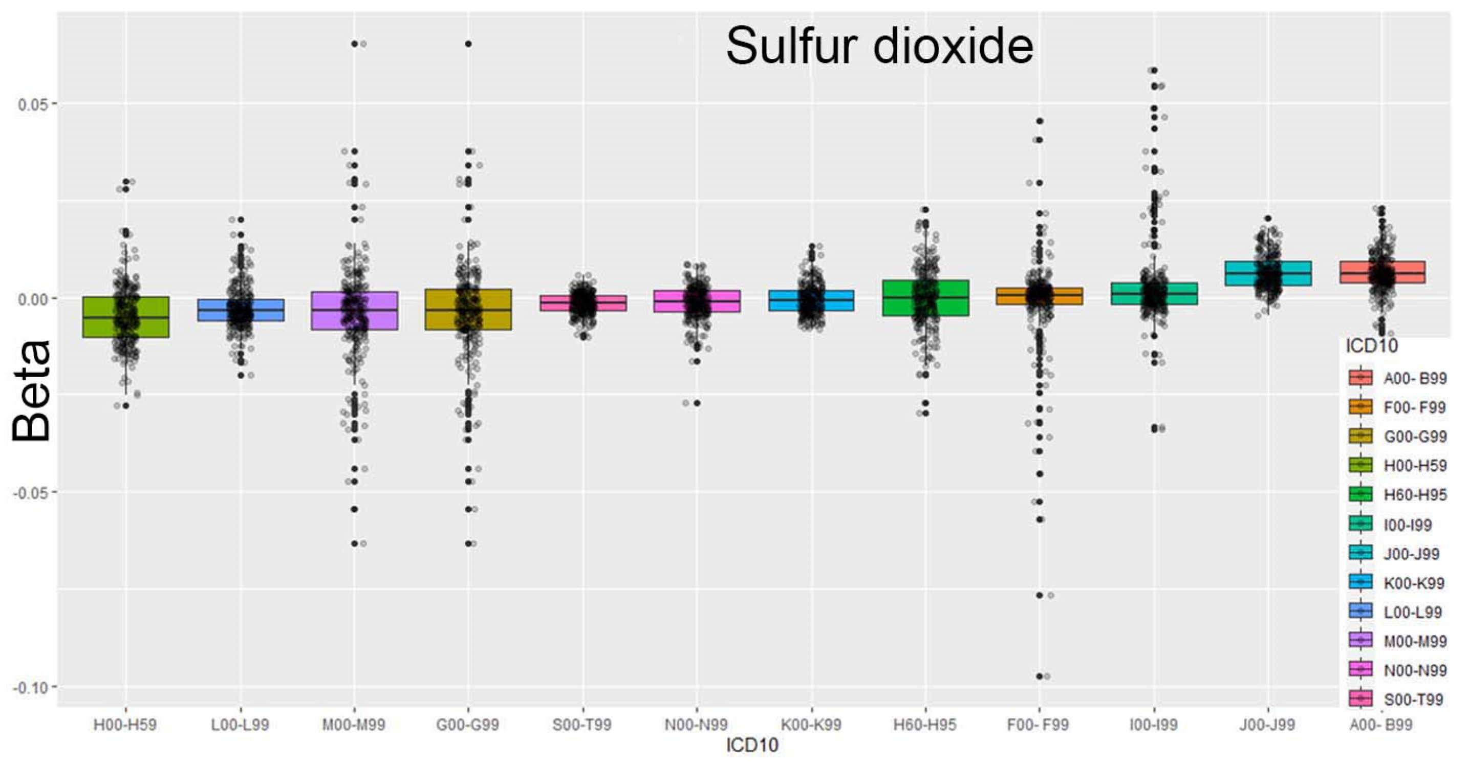
For each air pollutant, visualizations can be generated to explore potential correlations and trends. For instance, Figure 1 illustrates the case of sulfur dioxide concentrations, using a box plot to depict the data distribution. This plot presents the three quartiles, Q1 (25%), Q2 (50%, median), and Q3 (75%), with any data points outside this range identified as outliers.

In this analysis, the data were ordered according to ICD-10 codes, with the sorting criterion based on the median value.

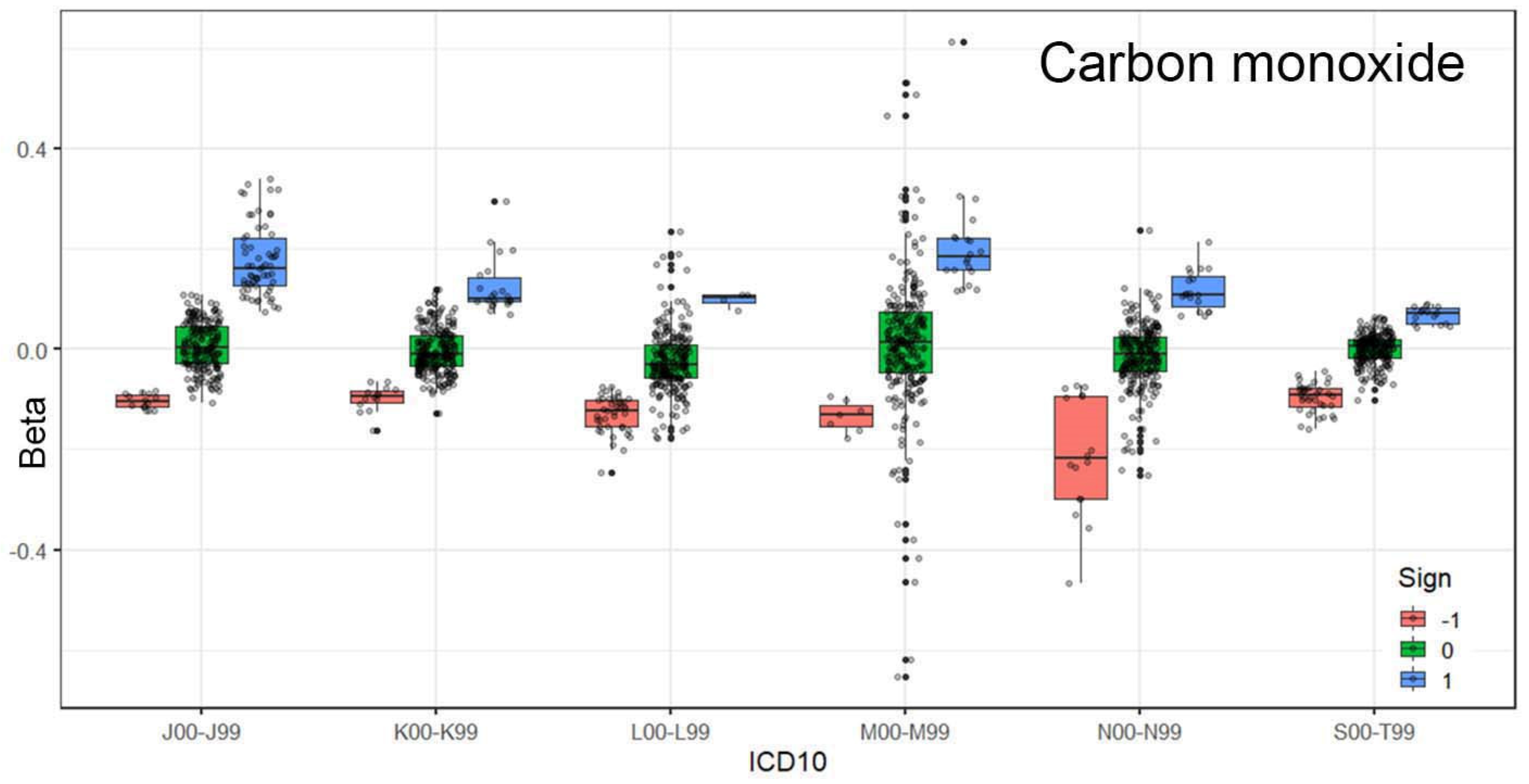
Figure 2 illustrates the relationships for carbon monoxide. The results are categorized into three cases: a statistically significant positive relationship (1), a negative relationship (−1), or no relationship (0). The association between carbon monoxide exposure and respiratory diseases is evident.

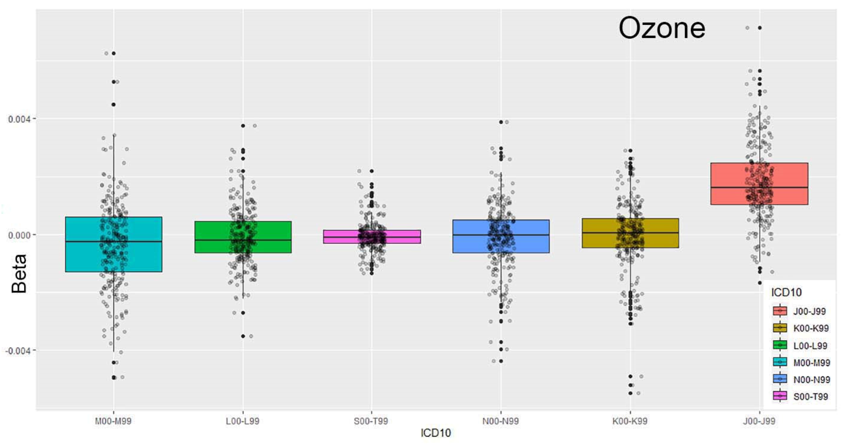
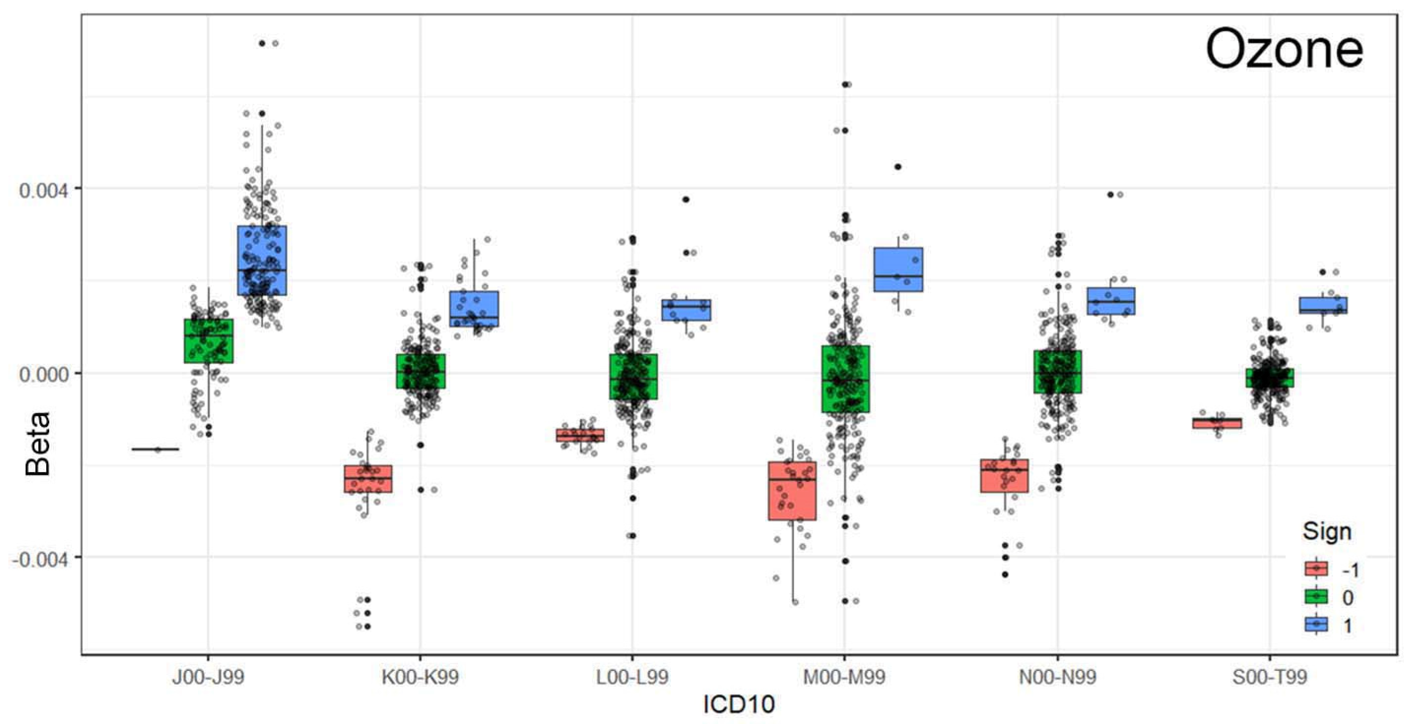
Figure 3 and Figure 4 illustrate the relationship between respiratory system conditions and exposure to ozone concentrations in the environment. The ordering of ICD-10 codes based on the median (Q2) highlights a strong association between ozone levels and emergency department (ED) visits for respiratory issues.

This is further confirmed by grouping the coefficients based on their statistical relationships (−1, 0, and 1). As shown in Figure 4, statistically significant positive relationships are the most prominent among the tested associations.

It is important to note that the data used in this study are derived from statistical models, enabling the observation of multiple relationships. For each air pollutant, we analyze 15 lag periods (lag 0–14 days). Each lagged exposure includes 18 strata, resulting in 18 pairs of values (Beta, SE).

Figure 5 illustrates the distribution of the obtained Beta values for ED visits classified under A00–B99, which correspond to “Certain infectious and parasitic diseases”.

For ozone, a strong association (Beta > 0) is observed at lags 0, 1, and 2 and subsequently at lags 8, 9, and 10. In contrast, the relationship between exposure to sulfur dioxide follows a different pattern. This example demonstrates how the proposed approach effectively captures various dependencies. The use of strata enables the selection of different subgroups of ED visits, enhancing the reliability of the results.

Figure 6 consists of four panels, showing the relative risk (RR) for a 10-unit increase in sulfur dioxide concentration across four ED visit classifications. It illustrates how the effects differ across specific health categories. The black line represents the RR, the blue line shows the lower bound, and the red line indicates the upper bound. The median values for these lines were calculated using the median of 18 RR values and their corresponding 95% confidence intervals (CIs). This leads to the derivation of an analytical formula for RR as a function of lag, representing previous exposure to air pollution. Figure 6 displays the RR values. For example, in the A00–B99 classification, a 4% increase in risk is observed for the same-day exposure (lag 0). A horizonal line for RR=1.00 is shown.

The data, R program, and example results are available at the following location: https://github.com/szyszkowiczm/TorontoEDAirMetaAnalysis (accessed on 13 May 2025). This repository allows for the verification of the presented results and offers the possibility to obtain coefficients for the RR model as a function of lag.

4. Discussion

In summary, the proposed methodology can be outlined as follows: For a specific health outcome (e.g., ED visits for respiratory conditions), various strata are considered. This approach can be seen as sampling from the population of patients. In the present study, the analysis is conducted for all patients, as well as for males, females, and a total of 18 different subgroups. Some of these groups overlap (e.g., all patients and males). The strata are determined by age groups (0–10, 11–60, and above 60 years), sex (all, male, and female), and seasons (entire study period; cold season: October–March; warm season: April–September). These combinations result in 18 distinct groups of ED counts. For each group, the RR value is estimated. For example, using maximum among the estimated RR values gives the largest health effects.

From a policy perspective, it is crucial to determine the associations between pollutant concentrations and health outcomes. The proposed methodology allows for controlling the strength of these associations by using various percentiles of RRs and the corresponding 95% CIs. This technique can be applied to collect and assess associations estimated across multiple centers. Instead of combining or pooling effects (random or fixed), this approach allows for estimating the percentiles of risks from other studies.

One of the main findings of this study is the strong connection between respiratory diseases and exposure to air pollution. High concentrations of air pollution are associated with an increase in respiratory diseases. This finding supports previous results and observations published over many years [17,18,19]. Ozone has proven to be the most influential gas in terms of the number of ED visits related to respiratory diseases. Carbon monoxide also shows strong associations with these visits, suggesting that urban air is a major contributor to the worsening of respiratory conditions.

The result presented in Figure 1 is particularly interesting, as it reveals a link between infectious diseases and the presence of sulfur dioxide. Sulfur dioxide is an irritating gas that affects the eyes, skin, and especially the respiratory system. High levels can cause coughing, throat pain, and breathing difficulties and worsen asthma or heart conditions. It does not directly cause infections but weakens the respiratory tract, making it easier for infections to develop. Sulfur dioxide can also react with other compounds in the atmosphere to form fine particles in the air that reach deep into the lungs and cause similar health problems. The available data allow for various perspectives on the relationships between ED visits and specific pollutants.

Of course, more detailed results can be obtained by considering individual strata within the defined categories. For instance, closer examination can be made of relationships for children, the elderly, or based on seasonal variations.

A limitation of this study is that not all ED visits are considered, specifically not all 22 ICD-10 classifications. Many diseases are clearly not linked to air quality, and for these diseases, results should fall into the 0 category. However, the proposed approach can still capture other relationships and serve as a method of verification. For example, pre-arranged ED visits (e.g., for chemotherapy) should show no correlation with air pollution.

This study addresses several key issues related to research on the impact of air pollution on health. It assumes that there is good access to databases related to air quality and meteorological factors such as temperature, humidity, and others. Of course, having accurate health data is crucial. In this case, we refer to properly diagnosed emergency visits. Having extensive data over a long period, such as several years, is highly beneficial for obtaining reliable results.

Currently used statistical methods are highly effective. The application of the time-stratified case-crossover method allows for consistent control of time-related changes, such as seasonal, trend, and other variations. Thus, the computational process does not pose a significant challenge.

This study proposes analyzing all disease groups, meaning that calculations should be performed for all ICD-10 categories. As a result, one obtains a cube of results with components (stratum, air pollution/lag, ICD-10 code). This set of results enables the comprehensive exploration of the relationships between air pollution and health. It challenges the preconceived notion that air pollution only affects the respiratory system. In different centers, cities, or regions, the impact may vary significantly. Conducting such calculations will eliminate surprises regarding the associations between health and air quality.

The main objective of this study is to present an approach for summarizing results generated across various strata and lags. In conventional meta-analyses, results from different studies and locations are typically synthesized into a single estimate or a concentration–response function [20,21]. In this study, the proposed technique is applied to stratified estimations. This method allows for controlling the strength of associations.

As was already discussed, air pollution poses a serious threat to public health, contributing to respiratory, cardiovascular, and neurological diseases and many other health conditions. However, the adverse effects of air pollutants such as particulate matter, nitrogen dioxide, ozone, and other air pollutants in the urban environment are often not immediate. To account for the delayed onset of these effects, researchers frequently use distributed lag models (DLMs). This approach allows researchers to understand both the magnitude and timing of the health impact, providing a more comprehensive risk assessment [22,23,24].

DLMs are statistical models that estimate the association between an exposure and a health outcome across a range of time lags. For example, in studying daily mortality or hospital admissions, a DLM can capture how exposure to ozone over several days—today, yesterday, or even a week ago—contributes to current health risks. This time-distributed perspective helps to reveal both the timing and persistence of pollutant-related health impacts.

An important extension of this approach is the ability to evaluate effects across different population subgroups, particularly by age, sex, and season. Studies have shown that children and older adults often experience different lag patterns and sensitivities to air pollution. Several studies have demonstrated that health outcomes related to air pollution differ significantly by age. For example, research has shown that elderly populations are more susceptible to delayed mortality due to long-term exposure, while younger groups may face immediate but less severe effects. DLMs make it possible to quantify and compare these age-specific vulnerability profiles.

More advanced models, like distributed lag nonlinear models (DLNMs), can further account for nonlinear exposure–response functions, enhancing our understanding of how risk varies with both concentration and time across subgroups [25,26]. In this paper, we extract the patterns of the associations among 18 strata and lag distribution (0–14 days).

It is known that certain visits are unrelated to air pollution, so pre-scheduled visits should demonstrate independence in the calculations. Such results serve as a test of the reliability of the conducted study.

5. Conclusions

A broad perspective on the harmfulness of air pollution allows for the recognition of significant connections. The impact of ozone on the human respiratory system is well known [27,28], and this relationship has been clearly demonstrated through the applied approach. It is evident that the connection is strong. Inhaled air serves as a wide entry point for pollutants into the body. The thesis presented in this study suggests that health responses can occur across any system in the human body. Behavior and its consequences (such as injuries) are also associated with poor air quality. It seems reasonable to conduct similar studies in other centers and locations.

The presented study proposes several new approaches for summarizing results from large amounts of estimations. It allows for identifying and extracting patterns in the associations. While this paper shows only a portion of the analysis, it does not provide results for all considered indexes (AQHI and AQHIX). Since the data and R program are available, various combinations can easily be tested.