Article

Enhancing PM2.5 Air Pollution Prediction Performance by Optimizing the Echo State Network (ESN) Deep Learning Model Using New Metaheuristic Algorithms

1
Department of GIS, School of Surveying and Geospatial Engineering, College of Engineering, University of Tehran, Tehran 14399-57131, Iran
2
Department of GIS, Faculty of Geodesy and Geomatics Engineering, K. N. Toosi University of Technology, Tehran 19967-15433, Iran
3
Department of Pathology, Microbiology, and Immunology, School of Veterinary Medicine, University of California, Davis, CA 95616, USA
*
Authors to whom correspondence should be addressed.
Urban Sci. 2025, 9(5), 138; https://doi.org/10.3390/urbansci9050138
Submission received: 12 March 2025 / Revised: 15 April 2025 / Accepted: 18 April 2025 / Published: 23 April 2025

Abstract

:
Air pollution presents significant risks to both human health and the environment. This study uses air pollution and meteorological data to develop an effective deep learning model for hourly PM2.5 concentration predictions in Tehran, Iran. This study evaluates efficient metaheuristic algorithms for optimizing deep learning model hyperparameters to improve the accuracy of PM2.5 concentration predictions. The optimal feature set was selected using the Variance Inflation Factor (VIF) and the Boruta-XGBoost methods, which indicated the elimination of NO, NO2, and NOx. Boruta-XGBoost highlighted PM10 as the most important feature. Wavelet transform was then applied to extract 40 features to enhance prediction accuracy. Hyperparameters and weights matrices of the Echo State Network (ESN) model were determined using metaheuristic algorithms, with the Salp Swarm Algorithm (SSA) demonstrating superior performance. The evaluation of different criteria revealed that the ESN-SSA model outperformed other hybrids and the original ESN, LSTM, and GRU models.

1. Introduction

The global economy’s rapid expansion, industrialization, and urbanization are exacerbating air pollution [1]. Among these pollutants, respirable fine particulate matter with a diameter of 2.5 μm or less (PM2.5) is a major contributor in most urban areas [2]. PM2.5 negatively impacts air quality [3], leading to adverse health outcomes, increased mortality rates, and significant economic losses [4,5,6]. The 2021 Global Burden of Disease (GBD) study highlighted poor air quality, particularly in low- and middle-income countries, as a key factor in the global disease burden [7,8]. Lelieveld et al. [9] indicated that air pollution’s impact on premature deaths is evident worldwide, and it is projected to double by 2050 across various countries, including Iran, Japan, the United States of America, China, Germany, and Russia.
Air quality in Iran, particularly in urban areas, has deteriorated significantly, diverging from global PM2.5 guidelines [10]. Tehran, the capital, suffers from severe air pollution due to inadequate public transportation, heavy traffic, and high population density [11]. In 2021, long-term exposure to PM2.5 accounted for about 1.2 million disability-adjusted life years (DALYs) in Iran, with approximately 182,951 DALYs lost in Tehran alone [12]. Kazemi et al. [13] also predicted that the cost of air pollution-related deaths will rise from USD 898 million in 2020 to USD 13,621 million by 2030.
Developing efficient and dynamic information systems to model, monitor, and predict pollutants, particularly particulate matter, is crucial for urban management and decision making. Predicting PM2.5 concentrations involves a complex, nonlinear computational process influenced by various air pollution characteristics and atmospheric features [14]. Previous studies indicate that machine learning and deep learning models perform well in predicting PM2.5 [2,15]. Notably, deep learning models excel at capturing complex, nonlinear, and interactive relationships within time series data of pollutants [16].
Machine learning advancements have been made for air pollution predictions, emphasizing reduced input data and increased computational efficiency [17,18]. Notable models include decision trees [19,20], support vector machines (SVM) [20,21,22], and artificial neural networks (ANNs) [23,24]. The rapid evolution of deep learning has introduced techniques such as deep belief networks (DBNs) [25], long short-term memory (LSTM) [26,27,28], and gated recurrent units (GRU) [29,30] for air pollution prediction. These models leverage deep neural networks to uncover nonlinear relationships in data through hierarchical features, enabling them to identify complex patterns and achieve high prediction accuracy [31]. In a study conducted by Masood and Ahmad [21], two SVM and ANN models were built using different air pollution and meteorological data from 2016 to 2018. The results showed ANN to be more accurate than SVM, with R = 0.8567 and R = 0.7301, respectively. In [30], a simple recurrent neural network (RNN), LSTM, and GRU deep learning models predicted daily PM2.5 concentrations in four major Indian cities using various atmospheric gases and meteorological data from 2018 to 2023, with GRU outperforming the other models in all cities.
By combining machine/deep learning models with optimization models, it is possible to achieve more accurate evaluations and predictions; because of the need for high calculation speeds and accuracy, these hybrid models have become an important tool in predicting air pollution concentrations [15,16]. For instance, in [31], a hybrid deep learning approach predicted daily PM2.5 concentrations in Yining and Beijing, China. This approach employed random forest for feature importance assessment, followed by a deep learning architecture that integrated one-dimensional convolution neural networks (CNN) for feature extraction, LSTM for sequence modeling, and an attention mechanism to weight input features. The Improved Chimpanzee Optimization Algorithm was also used to optimize the hyperparameters. The model demonstrated high efficiency, achieving R2 values of 0.895 and 0.964 for Yining and Beijing, respectively.
Deep learning models excel at predicting PM2.5 concentrations but are complex and have unstable training processes [32]. The Echo State Network (ESN), a new type of RNN, effectively processes time series data [32,33]. The ESN employs a fixed random hidden layer to capture the features of nonlinear and complex sequences while avoiding gradient descent issues during training [34]. This transforms input signals into a high-dimensional state space. The output weight is determined through simple linear regression, while other weights are generated randomly, significantly reducing the computational load and accelerating model convergence [35]. In [36], the authors used a combination model of the ESN model and the improved particle swarm optimization (IPSO) algorithm to predict PM2.5 concentrations. IPSO was used to optimize the ESN model’s hyperparameters. The IPSO-ESN model with RMSE 9.4961 performed better than the ESN and LSTM models, with RMSE values of 13.4753 and 33.5302, respectively.
A literature review indicates that new models, such as ESN, and their combination with optimization algorithms increase PM2.5 concentration prediction accuracy and generalizability. Hence, to enhance the accuracy and generalizability of the ESN model for predicting PM2.5 time series data, it is crucial to select optimal hyperparameters and design the hidden layer effectively [37,38]. Additionally, choosing relevant input features, such as air pollution and meteorological data that influence the PM2.5 concentration, is vital for developing an accurate prediction model [32,39]. Consequently, a high-accuracy model should be created with minimal input features. Given that air pollution time series data are often nonlinear, complex, and non-stationary [39,40], preprocessing techniques such as Wavelet transforms [41,42] and Fourier series [43] are employed to reduce complexity and mitigate noise.
This study aims to develop an efficient optimized hybrid deep learning model for hourly PM2.5 concentration predictions in Tehran, Iran, using air pollution and meteorological features from January 2019 to December 2023. Accurate pollutant predictions are crucial for preventing and controlling air pollution. To achieve this, optimal features were selected using the Variance Inflation Factor (VIF) and Boruta-XGBoost methods and Wavelet transform to enhance prediction accuracy and feature extraction. Unlike the other feature selection methods that focus on finding the minimal feature subset for prediction, potentially sacrificing accuracy, Boruta-XGBoost comprehensively assesses all features to identify genuinely relevant ones [44,45]. Optimal hyperparameters are essential for improving model performance and reliability. Unlike previous studies [36,46] that relied on random selection or trial-and-error to determine the hyperparameters and weights vectors of the ESN, our study utilizes efficient metaheuristic algorithms—the Arithmetic Optimization Algorithm (AOA) [47], Harris Hawks Optimization (HHO) [48], and Salp Swarm Algorithm (SSA) [49]—to find the optimal values. These algorithms achieve better or competitive results in solving engineering problems compared to others. Hyperparameter optimization studies have demonstrated the superior performance of the selected metaheuristic algorithms across diverse machine learning and deep learning models [39,50,51,52]. In Paryani et al. [53] and Marouane et al. [54], HHO outperformed other algorithms including the Genetic Algorithm (GA), Particle Swarm Optimization (PSO), the Gray Wolf Optimizer (GWO), and the Bat Algorithm (BA). Meanwhile, in Ge et al. [55], AOA outperformed the Grasshopper Optimization Algorithm (GOA), and, in Dogan et al. [56], SSA outperformed algorithms including PSO, HHO, and Artificial Bee Colony (ABC). Finally, the developed optimized models are compared to well-established models, including LSTM and GRU, to evaluate the proposed approach.
The contributions of this study are as follows. (1) The present study identified the crucial features for PM2.5 concentration predictions using VIF and Boruta-XGBoost, and it then extracted the optimal features from them using Wavelet transform. (2) It evaluated the performance of AOA, HHO, and SSA for the hyperparameter optimization of the ESN deep learning model and improved its accuracy. (3) This study compared and evaluated the ESN deep learning model to the two well-established machine learning models (LSTM and GRU) for PM2.5 concentration predictions. The rest of the article comprises the materials and methods (Section 2), results (Section 3), discussion (Section 4), and conclusion (Section 5).

2. Materials and Methods

2.1. Study Area and Data Used

Tehran, Iran’s largest city and capital, spans over 615 km2 and has a population exceeding 9.03 million, as illustrated in Figure 1. Located between 35°31′ and 35°57′ N latitude and 51°04′ and 51°47′ E longitude, Tehran plays a major role in Iran’s economy and industry. However, it faces serious air pollution challenges and is ranked among the most polluted cities globally [19]. Studies show that air-pollution-related mortality in Tehran is significant and alarming [13], especially considering the city’s population of around 9 million, which comprises over 10% of Iran’s total population. Tehran municipality has established 23 air pollution measuring stations, as shown in Figure 1, to monitor air pollution parameters, including ozone (O3), carbon monoxide (CO), nitrogen oxides (NOx), sulfur dioxide (SO2), and particulate matter (PM10 and PM2.5). Additionally, the Iran Meteorological Organization (IRM) has set up three synoptic measuring stations, also illustrated in Figure 1, to track meteorological parameters such as wind direction (WD), wind speed (WS), ambient temperature (TEMP), and rainfall (RAIN).
This study predicts PM2.5 concentrations by analyzing 11 air pollution and meteorological parameters: O3, CO, NO, NO2, NOx, SO2, PM10, WD, WS, TEMP, and RAIN. Meteorological data were obtained from the IRM as three-hourly averages from synoptic stations, while air pollution and PM2.5 data were collected hourly from Tehran municipality’s air pollution measuring stations. The study specifically targets PM2.5 concentration predictions for the Modarres station, which is noted as the most polluted location in terms of PM2.5. The statistical information, including the minimum (min), maximum (max), standard deviation (std), average (mean), and median for all parameters, is presented in Table 1.

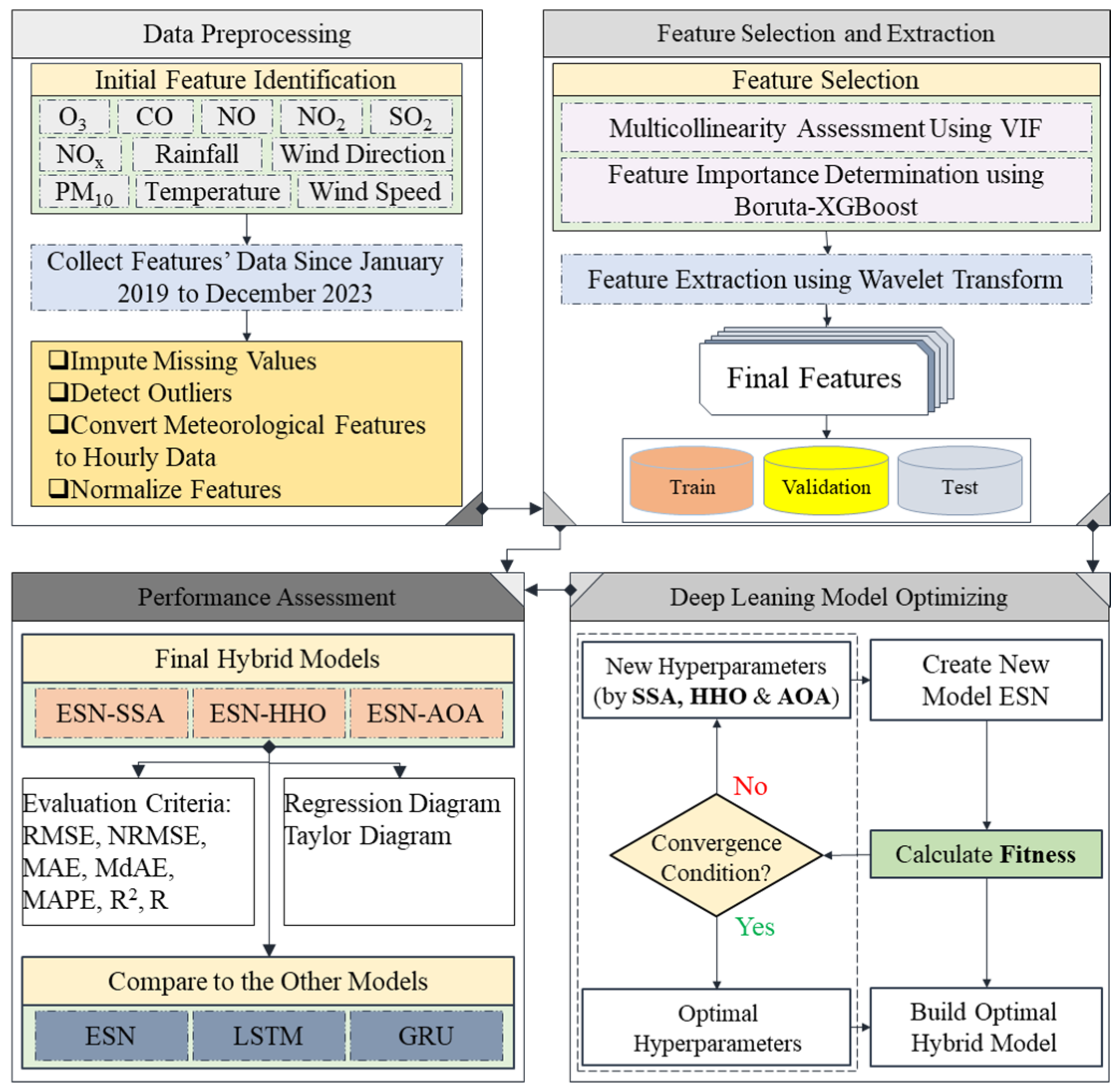
2.2. Proposed Methodology

This study uses a hybrid approach to predict PM2.5 concentrations in the Tehran metropolitan area. The key focus is on determining the hyperparameters and weights vectors of the ESN deep learning model. Unlike previous studies that relied on random selection or trial-and-error methods, this study employs a metaheuristic approach for the more accurate and efficient determination of hyperparameters and weights vectors. As Figure 2 and Algorithm 1 illustrate, the proposed methodology consists of four main steps: data preprocessing, feature selection and extraction, deep learning model optimizing, and performance assessment, which are detailed in the following sections.
Data Preprocessing: From January 2019 to December 2023, we collected hourly time series data on air pollution parameters and three-hourly time series on meteorological parameters influencing PM2.5 concentrations. The data were first cleaned by filling in missing values using Inverse Distance Weighted (IDW) and Linear Interpolation and identifying outliers with the mean and standard deviation [57]. Then, using linear interpolation, meteorological features were converted to hourly data. Subsequently, the Z-Score method was applied to normalize the time series data.
Feature selection and extraction: To address multicollinearity, the VIF value for each feature was calculated first, and features with high multicollinearity were eliminated. Boruta-XGBoost was then used to assess the importance of the remaining features after a VIF assessment and to identify the optimal combination influencing the PM2.5 concentration. In this study, Boruta-XGBoost served as an efficient method for evaluating features and selecting those that effectively predict PM2.5 concentrations. Wavelet transform was employed to analyze the non-stationary characteristics and dynamic signals of meteorological and air pollution features (selected features using Boruta-XGBoost), enhancing the accuracy of hourly PM2.5 concentration predictions. It extracts various components, such as seasonal trends, decomposes non-stationary signals across different time scales, and improves the interpretation of temporal variability. After the previous sub-steps, the data were categorized into training (2019–2021), validation (2022), and testing (2023) time series data.
Deep learning model optimizing: The ESN model predicted PM2.5 hourly concentrations. To enhance accuracy and efficiency, the optimal hyperparameters for the ESN model were determined using new metaheuristic algorithms: SSA, HHO, and AOA.
Performance assessment: In this step, the final hybrid models, ESN-SSA, ESN-HHO, and ESN-AOA, are evaluated using various criteria and compared to the original ESN, LSTM, and GRU models. Regression lines and Taylor diagrams are created to identify the best model for PM2.5 concentration predictions.
Algorithm 1. Pseudo-code of the proposed methodology.
1. Data Preprocessing
i.
Missing values imputation using IDW and linear interpolation
ii.
Outlier detection and removing using mean and standard deviation
iii.
Meteorological features conversion to hourly data using linear interpolation
iv.
Normalization using Z-Score method
2. Feature Selection
i.
Multicollinearity assessment using VIF
ii.
Feature selection using Boruta-XGBoost
3. Feature extraction using wavelet transform
4. For 1 to 200:
5. Execution of metaheuristic (SSA, HHO, AOA) operators
6. Model training
7. Calculate objective function (0.8 × RMSETraining + 0.2 × RMSEValidation)
8. Update best solution
9. End (end of metaheuristic algorithms)
10. Return the best solution (optimal hyperparameters and weights vectors)

2.3. Boruta-XGBoost

Boruta was introduced as a feature selection method by Kursa and Rudnicki [44]. This method is a random forest algorithm that gives the importance of features in numerical form. In the original version of Boruta, the used base machine learning method for determining the features’ importance is a random forest; if this method changes to the XGBoost machine learning algorithm [58,59], the developed method is called Boruta-XGBoost. Boruta-XGBoost first creates shadow features based on the original features. Shadow features are random versions of the original features that include noise. Then, using original and shadow features, the XGBoost model is trained and, based on its performance, the importance of each feature is calculated. If the importance of an original feature is greater than the most important shadow feature, that feature is inserted into the final features subset and selected as the effective feature. Instead of selecting a minimal feature set, this algorithm identifies all features related to the dependent variable, enhancing prediction accuracy [44].

2.4. ESN

ESN, a deep recurrent network introduced by Jaeger [60], excels in time series prediction and classification [61,62]. The ESN architecture, illustrated in Figure 3, comprises three layers: an input layer with K neurons, a reservoir layer with N neurons, and an output layer with L neurons, where L equals 1 for time series prediction.
Equations (1) and (2) are used to update the reservoir state x(t) at time t. u(t + 1) is the input data, W i n R N × K is the input weights matrix and W r e s R N × N is the reservoir weights matrix, both of which are generated randomly. α and f are the leakage rate and activation function, respectively. Equation (3) shows the output state update. Here, W o u t R L × ( N + K ) is the output weight matrix, which is solved via linear regression. Using linear regression instead of gradient descent increases the accuracy and speed of ESN compared to traditional RNN [63,64]. Moreover, using linear regression ensures a global optimum. Equation (4) is used to obtain w o u t : here, X and Y are the reservoir and target outputs, respectively. I and λ are the identity matrix and regularization parameter, respectively:
x ~ t + 1 = f w i n u t + 1 + w r e s x t + 1 ,
x t + 1 = 1 α x t + α x ~ ( t + 1 )
y t + 1 = w o u t x ( t + 1 )
W o u t = ( X T X + λ I ) 1 X T Y
The ESN model has four key hyperparameters, with the optimal tuning significantly enhancing accuracy [65]. These are: (1) dynamic reservoir size (NDR), which is based on the number of reservoir neurons and helps prevent overfitting; (2) the sparse degree (SD), which influences neurons connectivity and the state update rate; (3) spectral radius (ρ), which ensures model stability by defining internal neurons as echo functions; and (4) the input scale (IS), which refers to the input signal’s magnitude [37,63,65]. For further reading, see references [60,63,66].

2.5. Metaheuristic Algorithms

This study utilized novel population-based metaheuristic algorithms to tackle complex numerical optimization problems. These algorithms effectively combine global (exploration) and local (exploitation) searches, enhancing their ability to solve intricate optimization challenges [67,68]. The success of these methods is influenced by the selection of an appropriate population size and the number of optimization iterations, which can improve the likelihood of achieving a global optimum [69]. Various studies have shown them to be effective for optimal hyperparameter tuning [70,71,72,73]. Despite variations in the operators of different population-based metaheuristic algorithms, the core implementation steps in the optimization process remain consistent, as outlined in Algorithm 2.
Algorithm 2. Pseudo-code of metaheuristic algorithms for hyperparameter tuning
1. Inputs: the population size and maximum number of iterations
2. Outputs: the location of the best solution and its objective function value
3. Initial metaheuristic parameter (if needed)
4. Initial candidate solution
5. While (the stopping condition is not met) do:
    6. Execution of metaheuristic operators
    7. Calculating the objective function value
    8. Updating the best solution
9. End (end of metaheuristic algorithms)
10. Return the best solution

2.5.1. AOA

The AOA is a population-based metaheuristic algorithm based on the basic arithmetic operations’ distribution characteristics; it was developed by Abualigah et al. [47]. The arithmetic operations used in this algorithm include addition, subtraction, multiplication, and division [47]. In this algorithm, the two arithmetic operations of multiplication and division simulate the exploration phase and the two arithmetic operations of addition and subtraction simulate the exploitation phase [74]. In the exploration phase, the algorithm searches in the solution space extensively in order to avoid the local optimum solution; in order to enhance the quality of the achieved solutions in the exploration phase, the exploitation phase is considered [47]. The AOA algorithm selects the optimization strategy using the Math Optimizer Accelerated and, using derivative-free mathematical operators, it computes the best solution [75]. For more information, refer to the research conducted by Abualigah et al. [47].

2.5.2. HHO

The HHO is a swarm metaheuristic algorithm based on the cooperative behavior and chasing style of Harris hawks, introduced by Heidari et al. [48]. This algorithm is inspired by the cooperative hunting behavior of Harris hawks: specifically, their chasing and pouncing strategies. The HHO algorithm mathematically models Harris hawks’ behaviors, including their searches for prey, surprise pounces, and several attack strategies for hunting, to simulate exploration and exploitation [76]. This algorithm uses the escaping energy of the prey for the transition from exploration to exploitation. When this energy is increased (|E| ≥ 1), the exploration phase begins and the Harris hawks search in the solution space for the optimal solutions. When this energy is decreased (|E| < 1), the exploitation phase is instigated and the Harris hawks search for more accurate solutions in the neighborhood of the obtained solutions from the exploration phase. For more information, refer to Heidari et al. [48].

2.5.3. SSA

The SSA is a swarm metaheuristic algorithm based on salps’ swarming behaviors in the oceans, including navigating and foraging; it was introduced by Mirjalili et al. [49]. The population SSA is divided into two categories, including leader and followers, which models the salp chains and provides the mathematical form for problem solving. The leader, as a solution with a better performance rather than the followers, leads them to the optimal solution and the followers update their positions according to the leader, which is located in front of them. The position of the leader agent updates according to the food sources. These mechanisms simulate the exploration and exploitation phases in SSA. SSA uses a parameter to balance exploration and exploitation, where the exploration phase is performed in the earlier iterations while the exploitation is performed in the later iterations [77]. For more information, refer to Mirjalili et al. [49].

2.6. Evaluation Criteria

This study evaluates model performance using statistical criteria, including the mean absolute error (MAE), mean absolute percentage error (MAPE), median absolute error (MdAE), root mean square error (RMSE), normalized root mean square error (NRMSE), correlation coefficient (R), and coefficient of determination (R2) (Equations (5)–(11)). The lowest values of MAE, MAPE, MdAE, RMSE and NRMSE indicate the more accurate model, and the greatest values of R and R2 indicate the more accurate model. In the Equations (5)–(11), p i indicates the predicted PM2.5 concentration of the ith sample, m i indicates the observed PM2.5 concentration of the ith sample, n is the number of samples, S D p is the standard deviation of the predicted PM2.5 concentration of the all samples, p ¯ is the average of predicted PM2.5 concentration for the all samples, and m ¯ is the average of the observed PM2.5 concentration for the all samples:
M A E = m e a n p i m i ,
M A P E = 1 n i = 1 n p i m i p i ,
M d A E = m e d i a n p i m i ,
R M S E = 1 n i = 1 n ( p i m i ) 2 ,
N R M S E = R M S E S D p ,
R = i = 1 n ( m i m ¯ ) ( p i p ¯ ) i = 1 n ( m i m ¯ ) 2 i = 1 n ( p i p ¯ ) 2 ,
R 2 = 1 i = 1 n p i m i 2 i = 1 n m i m ¯ 2 ,

3. Results

In this section, the proposed methodology is implemented and its outcomes are presented.

3.1. Data Preprocessing

In the present study, data related to meteorological and air pollution parameters were obtained from sensors, and each parameter had missing values and outliers. The missing values must be imputed, and the outlier records must be identified and replaced. In order to address the imputation of missing values, we employ a hybrid approach that includes two phases: large-gap imputation and small-gap imputation. For a parameter, if the values are missing over a long time interval (large gap), measurement data for that parameter at nearby stations and the IDW method are used to impute the missing values. If the values are missing over a short time interval (small gap), measurement data for that parameter at the same station and linear interpolation are used to fill in the missing values. After imputing missing values, detecting and replacing outlier records is necessary. To identify outliers for a parameter, its mean (m) and standard deviation (std) are calculated. Any record falling outside the range [m – 3 × std, m + 3 × std] is considered an outlier and should be deleted and then replaced. As noted earlier, the meteorological data are collected every three hours. To convert these data to hourly data, we employed a method for small-gap imputation. The time series of the parameters after preprocessing is shown in Figure 4. Based on Figure 4, the trend of each parameter is determined over the course of the hour. For example, each year, there is a pattern of O3 changes with a high concentration in the middle of the year.

3.2. Feature Selection and Extraction

To eliminate irrelevant and correlated features for more accurate predictions and to avoid computational complexity, the selection of the best features is necessary. To this end, the VIF multicollinearity of the initial features (O3, CO, NO, NO2, NOx, SO2, PM10, WD, WS, TEMP, and RAIN) was calculated; then, features with VIF values greater than 10 were eliminated. Table 2 illustrates the VIF of the initial features; it is clear that the NO, NO2, and NOx features had a VIF greater than 10, so they were eliminated.
To select the best remaining features, we implemented Boruta-XGBoost with 400 trees and a maximum depth of 100. Figure 5 shows the feature importance that this method determined, where shadowMax represents the threshold below which features are eliminated. Since all features were of greater importance than shadowMax, none were deleted.
This study employed a Wavelet transform based on the parent “Haar” wavelet to extract new features from each original feature. Through trial and error, the maximum decomposition level was determined to be four, resulting in the decomposition of each feature into five new components: a4, d1, d2, d3, and d4. Consequently, each original feature in the dataset was replaced by these five new features. For instance, as depicted in Figure 6, the feature SO2 was decomposed into five new features (a4SO2, d1SO2, d2SO2, d3SO2, and d4SO2), which replaced the original SO2.

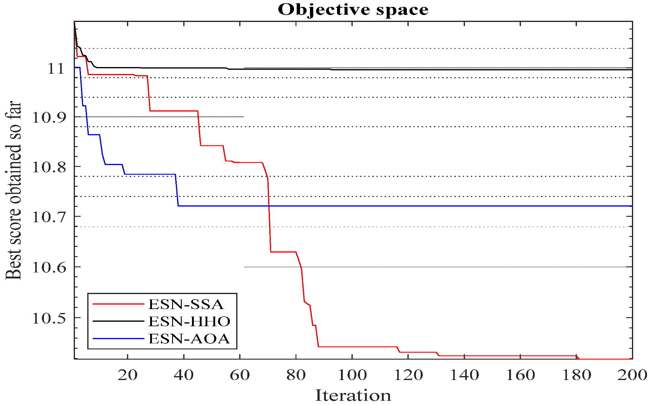
3.3. Deep Leaning Model Optimizing

This section implemented three metaheuristic algorithms to optimize the ESN hyperparameters—specifically, SD, ρ, IS, and the weights vectors Winput and Wreservoir. We determined the number of neurons in the reservoir layer to be 20 through trial and error. With 40 input features (eight original features, each decomposed into five new ones), Winput has a size of 800, and Wreservoir has a size of 400. Therefore, the total number of hyperparameters to optimize is 1203. Figure 7 depicts the convergence diagram of three metaheuristic algorithms—SSA, HHO, and AOA. All algorithms are implemented with 100 particles and 200 iterations. The SSA algorithm could more efficiently minimize the objective function value. This algorithm decreased the objective function from 11.0956 to 10.4192 and minimized it up to iteration 181. Meanwhile, the AOA and HHO algorithms converged after iterations 38 and 93, respectively. The HHO algorithm decreased the objective function from 11.0933 to 10.9958 and minimized it up to iteration 93. The AOA algorithm decreased the objective function from 11.008 to 10.7204 and minimized it up to iteration 38. The optimal values of the hyperparameters are presented in Table 3.

3.4. Performance Assessment

To evaluate the optimized hybrid models in this study, we also implemented the original ESN, GRU, and LSTM models, which are widely used in the literature. Table 4 outlines the evaluation criteria which presented in Section 2.6 for the three optimized models and the original ESN, GRU, and LSTM models. Overall, the ESN and its optimized hybrid version outperformed LSTM and GRU, with the original ESN performing better than both. In the training dataset, the ESN-SSA model demonstrated superior performance and generated more accurate predictions across all evaluation criteria, with significant differences compared to LSTM and GRU, showcasing the model’s capabilities. The ESN-AOA and ESN-HHO models also performed better than the others, though not as well as the ESN-SSA model. The ESN-SSA model excelled according to five evaluation criteria in the test dataset, while the ESN-HHO model performed best based on NRMSE and R. The ESN-SSA’s evaluation criteria showed significant differences compared to LSTM and GRU, reaffirming its capabilities. Similarly, the ESN-AOA, ESN-HHO, and ESN models performed better than the others, albeit with minor differences from the ESN-SSA model. To better understand the performance of the six models, Figure 8 presents the regression line diagram comparing predicted and observed PM2.5 values. The optimized and original ESN models outperformed the LSTM and GRU, with their predictions more closely aligned with the observed PM2.5 concentrations.
To statistically assess the similarity between the predicted and observed PM2.5 values and to identify the best prediction model for the training and test datasets, Taylor diagrams were prepared and are shown in Figure 9. In these diagrams, the model closest to the observed data is deemed the best for the given objective. The training and test datasets indicate that the optimized and original ESN models are closer to the observed values, while the LSTM and GRU models are not. Thus, the optimized and original ESN model predictions align more closely with the observed PM2.5 concentrations, particularly the ESN-SSA model.

4. Discussion

This study presents a comprehensive approach to predicting PM2.5 at Tehran’s most polluted air pollution station, with the aim of enhancing the performance of the deep learning model. The approach addresses all aspects of PM2.5 time series prediction, focusing on optimizing hyperparameters. It includes data preprocessing (imputation of missing values, outlier detection, and normalization), feature selection and extraction (multicollinearity assessment, and feature selection and extraction), hyperparameter optimization of the deep learning models, and performance assessment using various evaluation criteria and diagrams, with comparisons to established models.
The performance and reliability of deep learning models depend on well-chosen input features. This study utilized an integrated feature selection and extraction procedure to predict PM2.5 concentrations accurately. Initially, we assessed multicollinearity among the initial features and eliminated irrelevant ones; then, we identified the significance of the remaining features using Boruta-XGBoost. We applied Wavelet transform for feature extraction at four decomposition levels. Additionally, optimal hyperparameters enhance the model’s performance and reliability. Unlike previous studies [36,46] that determined the hyperparameters and weights vectors of the Echo State Network (ESN) through random selection or trial-and-error approaches, our study employs efficient metaheuristic algorithms to identify the optimal hyperparameters and weights vectors. The key results of this research are discussed below.
Previous studies identified 11 air pollution and meteorological parameters—O3, CO, NO, NO2, NOx, SO2, PM10, wind speed, wind direction, ambient temperature, and rainfall—as initial features. A multicollinearity assessment using VIF led to the elimination of NO, NO2, and NOx. Feature importance analysis with the Boruta-XGBoost method revealed that all the remaining features are significant, with PM10 being the most important, followed by SO2, CO, O3, rainfall, ambient temperature, wind speed, and wind direction. These results are consistent with Wei and Du [31], and Heidari et al. [39]. In other studies, features such as PM10, SO2, and CO are among the most important features and WD and WS are among the least important. However, in these two studies, ambient temperature was an important factor, but, in our study, it played a less important role. Through trial and error, the maximum decomposition level was set at 4, resulting in each feature being decomposed into five components via wavelet transform, yielding 40 extracted features.
To optimize the ESN model and determine the best hyperparameters SD, ρ, IS, and the weights vectors for the input and reservoir layers (Winput and Wreservoir), three metaheuristic algorithms—SSA, HHO, and AOA—were employed. The results indicated that the ESN-SSA hybrid model outperformed the others, followed by ESN-HHO and ESN-AOA. For additional insights, the original ESN, LSTM, and GRU models were also implemented and compared to the optimized hybrid models using various evaluation criteria. Since the ESN model avoids gradient descent during the training process and uses linear regression to obtain the output weights, it has a lower computational load and converges faster. According to this study, this issue was also demonstrated and is consistent with the studies of Chen and Zhang [32] and Xu and Ren [36]. The findings demonstrated that the optimized hybrid models significantly outperformed the three baseline models. Based on the results of this study and [22,31,36,39], where the optimization of hyperparameters improved the accuracy of PM2.5 concentration predictions, it can be concluded that combining machine learning models with optimization algorithms is a crucial step in predicting pollutant concentrations.
In this study, optimizing the ESN model’s hyperparameters and the input and reservoir neurons weights greatly influenced the prediction accuracy, which is consistent with the studies of Chen and Zhang [32] and Xu and Ren [36]. However, in the studies of Chen and Zhang [32] and Xu and Ren [36], reservoir weights are randomly generated, similarly to the simple ESN model. This can affect the model’s stability. This is because having optimal hyperparameters produces different results each time the model is trained due to the random generation of reservoir weights values. In this study, adding the reservoir weights along with other hyperparameters in the optimization process creates a stable model.
Solutions derived from metaheuristic algorithms proved more effective than trial-and-error methods such as random search. As observed in this study and previous studies [22,31,36,39], hybrid models perform better than simple models in which the hyperparameters are adjusted in a trial-and-error manner. Given the time-consuming nature of hyperparameter optimization, it is crucial to select a suitable metaheuristic algorithm that excels in terms of optimization accuracy and convergence speed. After evaluating three top metaheuristic algorithms in this study, SSA was chosen as the most effective.
This study is limited by the inadequate number and spatial distribution of the meteorological stations, which negatively impacts PM2.5 concentration prediction accuracy. In addition, the PM2.5 concentration was predicted only for the most polluted station in Tehran. While predicting PM2.5 concentrations for all stations would be more informative and effective for decision making, it is considerably more complex and time consuming.

5. Conclusions

This study investigated PM2.5 concentrations in Tehran, Iran, utilizing a comprehensive approach that incorporates Boruta-XGBoost and wavelet transform for optimal feature selection and extraction, along with metaheuristic algorithms (SSA, HHO, AOA) to determine the best hyperparameters and weights vectors for an ESN deep learning model. It extracted 40 features from air pollution and meteorological data. The results indicate that using these metaheuristic algorithms significantly improves PM2.5 prediction accuracy, with ESN-SSA showing the best performance. The hybrid models outperform the original ESN, LSTM, and GRU models. This approach provides a reliable method for air pollution prediction that is beneficial for decision makers in monitoring and controlling pollution in Tehran. Future research can explore new effective metaheuristic algorithms for hyperparameter optimization, incorporate additional relevant features, and develop improved feature elimination, selection, and extraction methods.

Author Contributions

Conceptualization, I.Z. and A.J.; methodology, I.Z. and A.J.; software, I.Z. and A.J.; validation, I.Z. and A.J.; formal analysis, I.Z. and A.J.; investigation, I.Z. and A.J.; resources, I.Z. and A.J.; data curation, I.Z. and A.J.; writing—original draft preparation, I.Z. and A.J.; writing—review and editing, I.Z., A.J. and A.L.; visualization, I.Z. and A.J.; supervision, A.L.; project administration, A.L. All authors have read and agreed to the published version of the manuscript.

Funding

This research received no external funding.

Data Availability Statement

The datasets used and/or analyzed during the current study are available from the corresponding author on reasonable request.

Conflicts of Interest

The authors declare no conflicts of interest.

References

  1. Wang, Y.; Yao, L.; Xu, Y.; Sun, S.; Li, T. Potential Heterogeneity in the Relationship between Urbanization and Air Pollution, from the Perspective of Urban Agglomeration. J. Clean. Prod. 2021, 298, 126822. [Google Scholar] [CrossRef]
  2. Bai, K.; Li, K.; Sun, Y.; Wu, L.; Zhang, Y.; Chang, N.-B.; Li, Z. Global Synthesis of Two Decades of Research on Improving PM2.5 Estimation Models from Remote Sensing and Data Science Perspectives. Earth-Sci. Rev. 2023, 241, 104461. [Google Scholar] [CrossRef]
  3. Luan, T.; Guo, X.; Guo, L.; Zhang, T. Quantifying the Relationship between PM2.5 Concentration, Visibility and Planetary Boundary Layer Height for Long-Lasting Haze and Fog–Haze Mixed Events in Beijing. Atmos. Chem. Phys. 2018, 18, 203–225. [Google Scholar] [CrossRef]
  4. Chuang, K.-J.; Chan, C.-C.; Su, T.-C.; Lee, C.-T.; Tang, C.-S. The Effect of Urban Air Pollution on Inflammation, Oxidative Stress, Coagulation, and Autonomic Dysfunction in Young Adults. Am. J. Respir. Crit. Care Med. 2007, 176, 370–376. [Google Scholar] [CrossRef] [PubMed]
  5. Mills, N.L.; Donaldson, K.; Hadoke, P.W.; Boon, N.A.; MacNee, W.; Cassee, F.R.; Sandström, T.; Blomberg, A.; Newby, D.E. Adverse Cardiovascular Effects of Air Pollution. Nat. Clin. Pract. Cardiovasc. Med. 2009, 6, 36–44. [Google Scholar] [CrossRef]
  6. Wu, R.; Dai, H.; Geng, Y.; Xie, Y.; Masui, T.; Liu, Z.; Qian, Y. Economic Impacts from PM2.5 Pollution-Related Health Effects: A Case Study in Shanghai. Environ. Sci. Technol. 2017, 51, 5035–5042. [Google Scholar] [CrossRef]
  7. Global Burden of Disease Collaborative Network Global Burden of Disease Study 2019 (GBD 2019) Air Pollution Exposure Estimates 1990–2019; Institute for Health Metrics and Evaluation (IHME): Seattle, WA, USA, 2021. [CrossRef]
  8. Pandey, A.; Brauer, M.; Cropper, M.L.; Balakrishnan, K.; Mathur, P.; Dey, S.; Turkgulu, B.; Kumar, G.A.; Khare, M.; Beig, G. Health and Economic Impact of Air Pollution in the States of India: The Global Burden of Disease Study 2019. Lancet Planet. Health 2021, 5, e25–e38. [Google Scholar] [CrossRef]
  9. Lelieveld, J.; Evans, J.S.; Fnais, M.; Giannadaki, D.; Pozzer, A. The Contribution of Outdoor Air Pollution Sources to Premature Mortality on a Global Scale. Nature 2015, 525, 367–371. [Google Scholar] [CrossRef]
  10. IQAir. World Air Quality Report: Region & City PM2.5 Ranking 2022. Available online: https://www.greenpeace.org/static/planet4-india-stateless/2023/03/2fe33d7a-2022-world-air-quality-report.pdf (accessed on 21 February 2025).
  11. Faridi, S.; Bayat, R.; Cohen, A.J.; Sharafkhani, E.; Brook, J.R.; Niazi, S.; Shamsipour, M.; Amini, H.; Naddafi, K.; Hassanvand, M.S. Health Burden and Economic Loss Attributable to Ambient PM2.5 in Iran Based on the Ground and Satellite Data. Sci. Rep. 2022, 12, 14386. [Google Scholar] [CrossRef]
  12. GBD Compare. GBD Compare 2021. Available online: https://vizhub.healthdata.org/gbd-compare/ (accessed on 21 February 2025).
  13. Kazemi, Z.; Yunesian, M.; Hassanvand, M.S.; Daroudi, R.; Ghorbani, A.; Sefiddashti, S.E. Hidden Health Effects and Economic Burden of Stroke and Coronary Heart Disease Attributed to Ambient Air Pollution (PM2.5) in Tehran, Iran: Evidence from an Assessment and Forecast up to 2030. Ecotoxicol. Environ. Saf. 2024, 286, 117158. [Google Scholar] [CrossRef]
  14. Abbasi, M.T.; Alesheikh, A.A.; Jafari, A.; Lotfata, A. Spatial and Temporal Patterns of Urban Air Pollution in Tehran with a Focus on PM2.5 and Associated Pollutants. Sci. Rep. 2024, 14, 25150. [Google Scholar] [CrossRef] [PubMed]
  15. Anchan, A.; Shedthi, B.S.; Manasa, G. Models Predicting PM2.5 Concentrations—A Review. In Recent Advances in Artificial Intelligence and Data Engineering; Shetty, D.P., Shetty, S., Eds.; Advances in Intelligent Systems and Computing; Springer Singapore: Singapore, 2022; Volume 1386, pp. 65–83. ISBN 9789811633416. [Google Scholar]
  16. Zhou, S.; Wang, W.; Zhu, L.; Qiao, Q.; Kang, Y. Deep-Learning Architecture for PM2.5 Concentration Prediction: A Review. Environ. Sci. Ecotechnol. 2024, 21, 100400. [Google Scholar] [CrossRef] [PubMed]
  17. Feng, Y.; Ning, M.; Lei, Y.; Sun, Y.; Liu, W.; Wang, J. Defending Blue Sky in China: Effectiveness of the “Air Pollution Prevention and Control Action Plan” on Air Quality Improvements from 2013 to 2017. J. Environ. Manag. 2019, 252, 109603. [Google Scholar] [CrossRef] [PubMed]
  18. Zamani Joharestani, M.; Cao, C.; Ni, X.; Bashir, B.; Talebiesfandarani, S. PM2.5 Prediction Based on Random Forest, XGBoost, and Deep Learning Using Multisource Remote Sensing Data. Atmosphere 2019, 10, 373. [Google Scholar] [CrossRef]
  19. Rad, A.K.; Razmi, S.-O.; Nematollahi, M.J.; Naghipour, A.; Golkar, F.; Mahmoudi, M. Machine Learning Models for Predicting Interactions between Air Pollutants in Tehran Megacity, Iran. Alex. Eng. J. 2024, 104, 464–479. [Google Scholar] [CrossRef]
  20. Salehie, O.; Jamal, M.H.B.; Shahid, S. Characterization and Prediction of PM2.5 Levels in Afghanistan Using Machine Learning Techniques. Theor. Appl. Climatol. 2024, 155, 9081–9097. [Google Scholar] [CrossRef]
  21. Masood, A.; Ahmad, K. A Model for Particulate Matter (PM2.5) Prediction for Delhi Based on Machine Learning Approaches. Procedia Comput. Sci. 2020, 167, 2101–2110. [Google Scholar] [CrossRef]
  22. Liu, Z.; Huang, X.; Wang, X. PM2.5 Prediction Based on Modified Whale Optimization Algorithm and Support Vector Regression. Sci. Rep. 2024, 14, 23296. [Google Scholar] [CrossRef]
  23. Oprea, M.; Mihalache, S.F.; Popescu, M. Computational Intelligence-Based PM2.5 Air Pollution Forecasting. Int. J. Comput. Commun. Control 2017, 12, 365–380. [Google Scholar] [CrossRef]
  24. Shah, J.; Mishra, B. Analytical Equations Based Prediction Approach for PM2.5 Using Artificial Neural Network. SN Appl. Sci. 2020, 2, 1516. [Google Scholar] [CrossRef]
  25. Xie, X.; Semanjski, I.; Gautama, S.; Tsiligianni, E.; Deligiannis, N.; Rajan, R.T.; Pasveer, F.; Philips, W. A Review of Urban Air Pollution Monitoring and Exposure Assessment Methods. ISPRS Int. J. Geo-Inf. 2017, 6, 389. [Google Scholar] [CrossRef]
  26. Zhao, L.; Li, Z.; Qu, L. A Novel Machine Learning-Based Artificial Intelligence Method for Predicting the Air Pollution Index PM2.5. J. Clean. Prod. 2024, 468, 143042. [Google Scholar] [CrossRef]
  27. Peng, L.; Zhu, Q.; Lv, S.-X.; Wang, L. Effective Long Short-Term Memory with Fruit Fly Optimization Algorithm for Time Series Forecasting. Soft Comput. 2020, 24, 15059–15079. [Google Scholar] [CrossRef]
  28. Wang, Z.; Crooks, J.L.; Regan, E.A.; Karimzadeh, M. High-Resolution Estimation of Daily PM2.5 Levels in the Contiguous US Using Bi-LSTM with Attention. Remote Sens. 2025, 17, 126. [Google Scholar] [CrossRef]
  29. Kim, Y.; Park, S.-B.; Lee, S.; Park, Y.-K. Comparison of PM2.5 Prediction Performance of the Three Deep Learning Models: A Case Study of Seoul, Daejeon, and Busan. J. Ind. Eng. Chem. 2023, 120, 159–169. [Google Scholar] [CrossRef]
  30. Govande, A.; Attada, R.; Shukla, K.K. Predicting PM2.5 Levels over Indian Metropolitan Cities Using Recurrent Neural Networks. Earth Sci. Inform. 2025, 18, 1–16. [Google Scholar] [CrossRef]
  31. Wei, M.; Du, X. Apply a Deep Learning Hybrid Model Optimized by an Improved Chimp Optimization Algorithm in PM2.5 Prediction. Mach. Learn. Appl. 2025, 19, 100624. [Google Scholar] [CrossRef]
  32. Chen, X.; Zhang, H. Grey Wolf Optimization–Based Deep Echo State Network for Time Series Prediction. Front. Energy Res. 2022, 10, 858518. [Google Scholar] [CrossRef]
  33. Na, X.; Han, M.; Ren, W.; Zhong, K. Modified BBO-Based Multivariate Time-Series Prediction System with Feature Subset Selection and Model Parameter Optimization. IEEE Trans. Cybern. 2020, 52, 2163–2173. [Google Scholar] [CrossRef]
  34. Qiao, J.; Li, F.; Han, H.; Li, W. Growing Echo-State Network with Multiple Subreservoirs. IEEE Trans. Neural Netw. Learn. Syst. 2016, 28, 391–404. [Google Scholar] [CrossRef]
  35. Yang, C.; Yang, S.; Tang, J.; Li, B. Design and Application of Adaptive Sparse Deep Echo State Network. IEEE Trans. Consum. Electron. 2023, 70, 3582–3592. [Google Scholar] [CrossRef]
  36. Xu, X.; Ren, W. Application of a Hybrid Model Based on Echo State Network and Improved Particle Swarm Optimization in PM2.5 Concentration Forecasting: A Case Study of Beijing, China. Sustainability 2019, 11, 3096. [Google Scholar] [CrossRef]
  37. Yang, X.; Wang, L.; Chen, Q. An Echo State Network with Adaptive Improved Pigeon-Inspired Optimization for Time Series Prediction. Appl. Intell. 2025, 55, 443. [Google Scholar] [CrossRef]
  38. Chen, H.-C.; Wei, D.-Q. Chaotic Time Series Prediction Using Echo State Network Based on Selective Opposition Grey Wolf Optimizer. Nonlinear Dyn. 2021, 104, 3925–3935. [Google Scholar] [CrossRef]
  39. Heidari, A.A.; Akhoondzadeh, M.; Chen, H. A Wavelet PM2.5 Prediction System Using Optimized Kernel Extreme Learning with Boruta-XGBoost Feature Selection. Mathematics 2022, 10, 3566. [Google Scholar] [CrossRef]
  40. Zhu, S.; Lian, X.; Liu, H.; Hu, J.; Wang, Y.; Che, J. Daily Air Quality Index Forecasting with Hybrid Models: A Case in China. Environ. Pollut. 2017, 231, 1232–1244. [Google Scholar] [CrossRef]
  41. Xing, G.; Zhao, E.; Zhang, C.; Wu, J. A Decomposition-Ensemble Approach with Denoising Strategy for PM2.5 Concentration Forecasting. Discret. Dyn. Nat. Soc. 2021, 2021, 5577041. [Google Scholar] [CrossRef]
  42. Shu, Y.; Ding, C.; Tao, L.; Hu, C.; Tie, Z. Air Pollution Prediction Based on Discrete Wavelets and Deep Learning. Sustainability 2023, 15, 7367. [Google Scholar] [CrossRef]
  43. Yang, Z. Hourly Ambient Air Humidity Fluctuation Evaluation and Forecasting Based on the Least-Squares Fourier-Model. Measurement 2019, 133, 112–123. [Google Scholar] [CrossRef]
  44. Kursa, M.B.; Rudnicki, W.R. Feature Selection with the Boruta Package. J. Stat. Softw. 2010, 36, 1–13. [Google Scholar] [CrossRef]
  45. Xu, J.; Wei, Y.; Zeng, P. VMD-Based Iterative Boruta Feature Extraction and CNNA-BiLSTM for Short-Term Load Forecasting. Electr. Power Syst. Res. 2025, 238, 111172. [Google Scholar] [CrossRef]
  46. Liu, H.; Zhang, X. AQI Time Series Prediction Based on a Hybrid Data Decomposition and Echo State Networks. Environ. Sci. Pollut. Res. 2021, 28, 51160–51182. [Google Scholar] [CrossRef] [PubMed]
  47. Abualigah, L.; Diabat, A.; Mirjalili, S.; Abd Elaziz, M.; Gandomi, A.H. The Arithmetic Optimization Algorithm. Comput. Methods Appl. Mech. Eng. 2021, 376, 113609. [Google Scholar] [CrossRef]
  48. Heidari, A.A.; Mirjalili, S.; Faris, H.; Aljarah, I.; Mafarja, M.; Chen, H. Harris Hawks Optimization: Algorithm and Applications. Future Gener. Comput. Syst. 2019, 97, 849–872. [Google Scholar] [CrossRef]
  49. Mirjalili, S.; Gandomi, A.H.; Mirjalili, S.Z.; Saremi, S.; Faris, H.; Mirjalili, S.M. Salp Swarm Algorithm: A Bio-Inspired Optimizer for Engineering Design Problems. Adv. Eng. Softw. 2017, 114, 163–191. [Google Scholar] [CrossRef]
  50. Kayhomayoon, Z.; Naghizadeh, F.; Malekpoor, M.; Arya Azar, N.; Ball, J.; Ghordoyee Milan, S. Prediction of Evaporation from Dam Reservoirs under Climate Change Using Soft Computing Techniques. Environ. Sci. Pollut. Res. 2023, 30, 27912–27935. [Google Scholar] [CrossRef]
  51. Rezaie, F.; Panahi, M.; Bateni, S.M.; Lee, S.; Jun, C.; Trauernicht, C.; Neale, C.M. Development of Novel Optimized Deep Learning Algorithms for Wildfire Modeling: A Case Study of Maui, Hawai ‘i. Eng. Appl. Artif. Intell. 2023, 125, 106699. [Google Scholar] [CrossRef]
  52. Almalawi, A.; Khan, A.I.; Alsolami, F.; Alkhathlan, A.; Fahad, A.; Irshad, K.; Alfakeeh, A.S.; Qaiyum, S. Arithmetic Optimization Algorithm with Deep Learning Enabled Airborne Particle-Bound Metals Size Prediction Model. Chemosphere 2022, 303, 134960. [Google Scholar] [CrossRef]
  53. Paryani, S.; Bordbar, M.; Jun, C.; Panahi, M.; Bateni, S.M.; Neale, C.M.; Moeini, H.; Lee, S. Hybrid-Based Approaches for the Flood Susceptibility Prediction of Kermanshah Province, Iran. Nat. Hazards 2023, 116, 837–868. [Google Scholar] [CrossRef]
  54. Marouane, B.; Mu’azu, M.A.; Petroselli, A. Prediction of Reservoir Evaporation Considering Water Temperature and Using ANFIS Hybridized with Metaheuristic Algorithms. Earth Sci. Inform. 2024, 17, 1779–1798. [Google Scholar] [CrossRef]
  55. Ge, Q.; Li, C.; Yang, F. Support Vector Machine to Predict the Pile Settlement Using Novel Optimization Algorithm. Geotech. Geol. Eng. 2023, 41, 3861–3875. [Google Scholar] [CrossRef]
  56. Dogan, M.; Taspinar, Y.S.; Cinar, I.; Kursun, R.; Ozkan, I.A.; Koklu, M. Dry Bean Cultivars Classification Using Deep Cnn Features and Salp Swarm Algorithm Based Extreme Learning Machine. Comput. Electron. Agric. 2023, 204, 107575. [Google Scholar] [CrossRef]
  57. Junninen, H.; Niska, H.; Tuppurainen, K.; Ruuskanen, J.; Kolehmainen, M. Methods for Imputation of Missing Values in Air Quality Data Sets. Atmos. Environ. 2004, 38, 2895–2907. [Google Scholar] [CrossRef]
  58. Chen, T.; He, T.; Benesty, M.; Khotilovich, V.; Tang, Y.; Cho, H.; Chen, K.; Mitchell, R.; Cano, I.; Zhou, T. Xgboost: Extreme Gradient Boosting. R Package Version 0.4-2 2015, 1, 1–4. [Google Scholar]
  59. Friedman, J.H. Greedy Function Approximation: A Gradient Boosting Machine. Ann. Stat. 2001, 29, 1189–1232. [Google Scholar] [CrossRef]
  60. Jaeger, H. The “Echo State” Approach to Analysing and Training Recurrent Neural Networks-with an Erratum Note. Bonn Ger. Ger. Natl. Res. Cent. Inf. Technol. Gmd Tech. Rep. 2001, 148, 13. [Google Scholar]
  61. Rigamonti, M.; Baraldi, P.; Zio, E.; Roychoudhury, I.; Goebel, K.; Poll, S. Ensemble of Optimized Echo State Networks for Remaining Useful Life Prediction. Neurocomputing 2018, 281, 121–138. [Google Scholar] [CrossRef]
  62. Yusoff, M.-H.; Chrol-Cannon, J.; Jin, Y. Modeling Neural Plasticity in Echo State Networks for Classification and Regression. Inf. Sci. 2016, 364, 184–196. [Google Scholar] [CrossRef]
  63. Ozturk, M.C.; Xu, D.; Principe, J.C. Analysis and Design of Echo State Networks. Neural Comput. 2007, 19, 111–138. [Google Scholar] [CrossRef]
  64. Sun, C.; Song, M.; Hong, S.; Li, H. A Review of Designs and Applications of Echo State Networks. arXiv 2020, arXiv:2012.02974. [Google Scholar] [CrossRef]
  65. He, K.; Mao, L.; Yu, J.; Huang, W.; He, Q.; Jackson, L. Long-Term Performance Prediction of PEMFC Based on LASSO-ESN. IEEE Trans. Instrum. Meas. 2021, 70, 1–11. [Google Scholar] [CrossRef]
  66. Jaeger, H. Echo State Network. Scholarpedia 2007, 2, 2330. [Google Scholar] [CrossRef]
  67. Marino, R.; Kirkpatrick, S. Hard Optimization Problems Have Soft Edges. Sci. Rep. 2023, 13, 3671. [Google Scholar] [CrossRef]
  68. Kirkpatrick, S.; Gelatt, C.D., Jr.; Vecchi, M.P. Optimization by Simulated Annealing. Science 1983, 220, 671–680. [Google Scholar] [CrossRef]
  69. Mirjalili, S. SCA: A Sine Cosine Algorithm for Solving Optimization Problems. Knowl.-Based Syst. 2016, 96, 120–133. [Google Scholar] [CrossRef]
  70. Alesheikh, A.A.; Chatrsimab, Z.; Rezaie, F.; Lee, S.; Jafari, A.; Panahi, M. Land Subsidence Susceptibility Mapping Based on InSAR and a Hybrid Machine Learning Approach. Egypt. J. Remote Sens. Space Sci. 2024, 27, 255–267. [Google Scholar] [CrossRef]
  71. Jafari, A.; Alesheikh, A.A.; Zandi, I.; Lotfata, A. Spatial Prediction of Human Brucellosis Susceptibility Using an Explainable Optimized Adaptive Neuro Fuzzy Inference System. Acta Trop. 2024, 260, 107483. [Google Scholar] [CrossRef]
  72. Yousefi, Z.; Alesheikh, A.A.; Jafari, A.; Torktatari, S.; Sharif, M. Stacking Ensemble Technique Using Optimized Machine Learning Models with Boruta–XGBoost Feature Selection for Landslide Susceptibility Mapping: A Case of Kermanshah Province, Iran. Information 2024, 15, 689. [Google Scholar] [CrossRef]
  73. Jafari, A.; Alesheikh, A.A.; Rezaie, F.; Panahi, M.; Shahsavar, S.; Lee, M.-J.; Lee, S. Enhancing a Convolutional Neural Network Model for Land Subsidence Susceptibility Mapping Using Hybrid Meta-Heuristic Algorithms. Int. J. Coal Geol. 2023, 277, 104350. [Google Scholar] [CrossRef]
  74. Kaveh, A.; Hamedani, K.B. Improved Arithmetic Optimization Algorithm and Its Application to Discrete Structural Optimization; Elsevier: Amsterdam, The Netherlands, 2022; Volume 35, pp. 748–764. [Google Scholar]
  75. Hu, G.; Zhong, J.; Du, B.; Wei, G. An Enhanced Hybrid Arithmetic Optimization Algorithm for Engineering Applications. Comput. Methods Appl. Mech. Eng. 2022, 394, 114901. [Google Scholar] [CrossRef]
  76. Zhang, M.; Chen, H.; Heidari, A.A.; Chen, Y.; Wu, Z.; Cai, Z.; Liu, L. WHHO: Enhanced Harris Hawks Optimizer for Feature Selection in High-Dimensional Data. Clust. Comput. 2025, 28, 186. [Google Scholar] [CrossRef]
  77. Bilal, O.; Asif, S.; Zhao, M.; Khan, S.U.R.; Li, Y. An Amalgamation of Deep Neural Networks Optimized with Salp Swarm Algorithm for Cervical Cancer Detection. Comput. Electr. Eng. 2025, 123, 110106. [Google Scholar] [CrossRef]
Figure 1. Study area.
Urbansci 09 00138 g001
Figure 2. The proposed methodology.
Urbansci 09 00138 g002
Figure 3. The general structure of ESN.
Urbansci 09 00138 g003
Figure 4. Time series of used data, separated by parameters and by hour.
Urbansci 09 00138 g004
Figure 5. The determined features’ importance according to the Boruta-XGBoost method.
Urbansci 09 00138 g005
Figure 6. Decomposing SO2 into five new features: a4SO2, d1SO2, d2SO2, d3SO2, and d4SO2.
Urbansci 09 00138 g006
Figure 7. Convergence diagram of three metaheuristic algorithms—SSA, HHO, and AOA.
Urbansci 09 00138 g007
Figure 8. The regression line diagrams for (a) ESN, (b) ESN-SSA, (c) ESN-HHO, (d) ESN-AOA, (e) LSTM and (f) GRU.
Urbansci 09 00138 g008
Figure 9. Taylor diagrams for training and test datasets for (a) the training data and (b) the test data.
Urbansci 09 00138 g009
Table 1. Statistical information of all parameters.
IndexO3
(ppb)
CO
(ppm)
NO
(ppb)
NO2
(ppb)
NOx
(ppb)
SO2
(ppb)
Min.−6.06−0.02−10.831.922.370.10
Max.213.0320.96983.53173.081093.01190.71
Std.24.841.54102.8823.07116.844.71
Mean21.871.9068.9747.88116.605.52
Median9.601.4224.5647.1076.404.43
IndexPM10
(μg/m3)
WD
(c°)
WS
(m/s)
TEMP
(°C)
RAIN
(mm)
PM2.5
(μg/m3)
Min.1.500.000.000.001.000.33
Max.1654.5097.009.009.009.00293.60
Std.50.9115.102.851.520.8921.65
Mean79.0310.302.541.161.7532.76
Median71.295.001.430.761.6727.00
Table 2. The VIF of the initial features.
FeaturesVIFFeaturesVIF
O31.82PM101.38
CO8.91WD1.23
NO745.07WS2.51
NO242.39TEMP2.47
NOx971.67RAIN1.05
SO21.23
Table 3. Optimal values of the hyperparameters.
HyperparameterAOAHHOSSA
Sparse degree0.10000.10020.1001
Spectral Radios0.23230.10000.8464
Input scaling0.32540.19670.1003
Table 4. The evaluation criteria for all models.
Model (Train)RMSERankNRMSERankMAERankMdAERankMAPERankR2RankRRank
LSTM19.450053.0838612.274256.781150.350950.110850.71555
GRU19.618462.4687512.806067.586660.352360.095360.71466
ESN11.533440.674548.522446.494540.335640.687340.82914
ESN-SSA10.395510.569117.583415.648810.304010.746010.86401
ESN-HHO11.018030.629638.101836.144630.321330.714730.84543
ESN-AOA10.754620.603927.928326.037320.317520.728120.85342
Model (Test)RMSERankNRMSERankMAERankMdAERankMAPERankR2RankRRank
LSTM22.162363.2319613.823857.308540.330340.092860.73165
GRU22.144852.6652514.051567.736550.328830.094250.72246
ESN15.159840.5695310.411447.879760.338160.575540.83033
ESN-SSA13.750310.567529.514916.826210.312310.650810.83532
ESN-HHO14.704530.5520110.142037.566430.332250.600630.84111
ESN-AOA14.612120.588449.871527.093720.316520.605620.81974
Disclaimer/Publisher’s Note: The statements, opinions and data contained in all publications are solely those of the individual author(s) and contributor(s) and not of MDPI and/or the editor(s). MDPI and/or the editor(s) disclaim responsibility for any injury to people or property resulting from any ideas, methods, instructions or products referred to in the content.

