Article

Impact of COVID-19 Restrictions and Traffic Intensity on Urban Stormwater Quality in Denver, Colorado

by
Khaled A. Sabbagh
1,*,
Pablo Garcia-Chevesich
1,2,* and
John E. McCray
1,3,4
1
Department of Civil and Environmental Engineering, Colorado School of Mines, Golden, CO 80401, USA
2
Intergovernmental Hydrological Programme, United Nations Educational, Scientific and Cultural Organization (UNESCO), Luis Piera 1992, Edificio Mercosur, 2do piso, Monevideo 11200, Uruguay
3
ReNUWIt National Science Foundation Engineering Research Center for Urban Water, Golden, CO 80401, USA
4
Hydrologic Science and Engineering Program, Colorado School of Mines, Golden, CO 80401, USA
*
Authors to whom correspondence should be addressed.
Urban Sci. 2025, 9(3), 81; https://doi.org/10.3390/urbansci9030081
Submission received: 23 January 2025 / Revised: 5 March 2025 / Accepted: 10 March 2025 / Published: 12 March 2025

Abstract

:
Urban stormwater may contain pollutants from different traffic vehicular sources including brake and tire wear, exhaust emissions, and atmospheric deposition. In this research, we took advantage of COVID-19 restrictions to evaluate the effects of historically low vehicular circulation on stormwater quality (metal concentrations and mass loads) generated from an urban watershed in Denver (Colorado). The analysis was performed at different hydrograph stages, i.e., first flush, peak flow, and recession stages during and after the imposition of the COVID-19 restrictions. Metal concentrations were compared with the maximum contaminant levels (MCLs) defined by the US Environmental Protection Agency (EPA) for drinking water as an indicator of water quality degradation. The results indicate that the Fe and Mn levels were constantly above the MCLs in stormwater, while then level of Pb occasionally surpassed the limits. Additionally, the highest pollutant mass loads generally occurred during peak flow conditions. Importantly, there was a clear effect of COVID-19 restrictions, suggesting that more stormwater pollution occurred after the restrictions were lifted, as a result of more vehicles circulating. Considering local climate, the mass loads of Fe, Mn, and Pb (the pollutants of concern) were estimated to be 0.4489, 0.0772, and 0.00032 MT/year, respectively, which are similar to loads reported in the literature for cities with similar climates and development levels.

1. Introduction

Urban water pollution involves surface runoff contaminants, contributing to various environmental and public health issues (e.g., [1]). This pollution is affected by many factors including physical (land use, soil type, topography) (e.g., [2,3,4]), biological (presence of microorganisms) (e.g., [5]), and chemical (heavy metals, petroleum products, pesticides, and fertilizers) (e.g., [6]). Vehicular traffic (i.e., the number of vehicles circulating in a given time) can be a significant source of stormwater pollution [7] and can seriously impact the water quality downstream of urban areas [8,9], as vehicular sources emit hazardous contaminants, mainly from exhaust fumes, fluid leaks, and wear of the drive train and brakes [10]. For a more detailed review of sources of traffic-related metals (as well as other pollutants) in urban stormwater, see [9].
Worldwide, numerous authors have evaluated the effects of vehicular traffic (e.g., [11,12,13]) on stormwater quality, suggesting that traffic pollutants in stormwater deteriorate surface water quality [13], causing potential injury to aquatic species [14] and the destruction of ecosystems [15]. Studies in Denver (Colorado) have documented metal pollution in stormwater and urban streams [16], but did not evaluate the importance of traffic as a pollutant source. Gustafson et al. [17], for example, evaluated the effects of urban redevelopment on stormwater quality in this North American city, concluding that phosphorous (P), nitrogen (N), copper (Cu), Zn, and total dissolved solids (TDS) concentrations are higher in recently redeveloped areas than previously reported values. Similarly, Pilone et al. [18] investigated the extent and sources of dry weather stream water quality in Denver, correlating urban catchment characteristics and pollution, concluding that nutrients and some metals were positively correlated with the imperviousness of land surfaces.
Heavy metals are well-known environmental contaminants because of their toxicity and long-term environmental persistence [19]. Specifically, Cu, Mn, Pb, Zn, and nickel (Ni) are known to be highly toxic [20]. For example, Fe contamination is toxic to D. Magna [21], while Mn can affect the immune defenses, perception of food, and normal muscle extension of crustaceans [22] and contribute to apoptosis and liver damage in fish due to oxidative stress [23]. Drinking water rich in Mn may affect the cognitive development of school-age children [24], while excess Fe may cause irritation in the eyes and skin, as well as liver cancer [25]. Similarly, Zn has negative effects on aquatic insect metamorphosis [26], while Pb may induce synaptic damage and neurotransmitter malfunction in fish due to oxidative stress [27]. Moreover, drinking water rich in Pb and Zn can cause carcinogenesis and non-carcinogenesis risk in children [28].
Metals have been found to enter urban surface water systems from vehicular sources such as automobiles, buses, and trucks (e.g., [29]). Concentrations of metals such as Pb, Cu, Cr, and Ni are thought to increase with more vehicular traffic (e.g., [30]). Even though vehicular traffic has been linked to some air quality parameters in Denver (e.g., [31]), potential links between traffic intensity and stormwater quality in this city are currently unknown, likely because it is challenging to evaluate the impact of traffic in an urban area with consistently high vehicular activity (e.g., [32]). However, during the enforcement of the COVID-19 restrictions, all activities (industrial, commercial, business, and transportation) nearly ceased in Denver, leading to urban traffic decreasing to historically low levels [33], providing a unique opportunity to investigate the effects of pollution generated from vehicular traffic on stormwater quality. In this study, traffic information was used to evaluate the possible effects of different traffic intensities on stormwater quality (metals) in Denver. Our hypothesis was that the lower traffic intensity due to the COVID-19 restrictions had a measurable influence on stormwater quality in this semiarid metropolitan area.

2. Materials and Methods

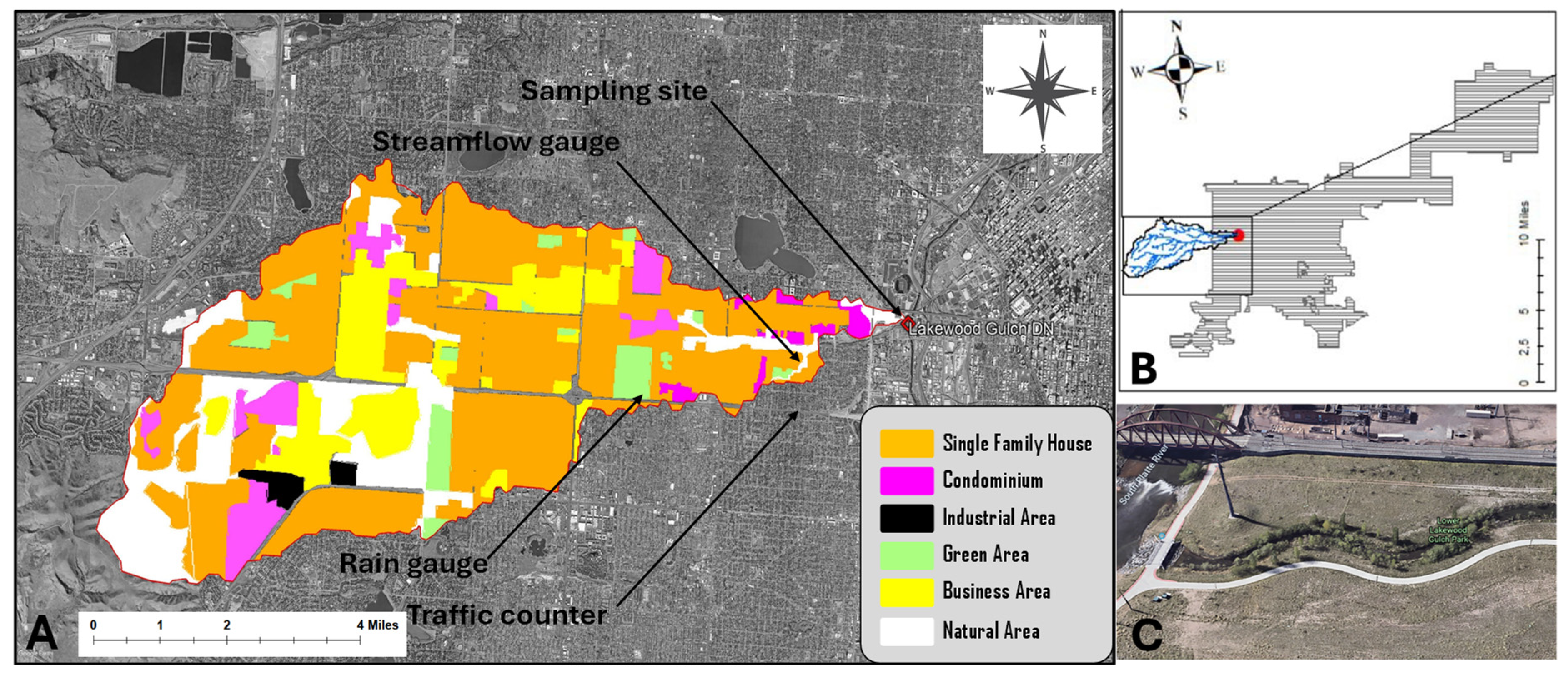
2.1. Study Site and Metal Selection

The South Platte River is the primary river in the Denver metropolitan area and is the city’s primary source of drinking water. For this research, the Lakewood Gulch (LG) watershed was selected because of its high traffic level, urban land use, accessibility, and availability of an upstream flow measurement. The drainage area is 3354 ha, with an average watershed slope of 6.5% [18]. Land uses in LG include roads (11%), industrial (1%), residential (52%), green (4%), business (14%), and natural (18%) areas. The geographical location, precipitation and streamflow gauges, stream network, and stormwater sampling site are shown in Figure 1. Based on data from the nearest meteorological station in Denver (1700, Cherry Creek at Champa by Urban Drainage and Flood Control District’s Nova Star 4.0 base station), the average daily air temperature ranges between −5.5 and 31.7 °C, being rarely below −14.4 °C or above 35.6 °C. Denver’s average annual rainfall and snowfall are 363 and 1370 mm, respectively [34].
The most common pollutants emitted from traffic vehicles (Cu, Fe, Ni, Pb, barium (Ba), Mn, and chromium (Cr)) (e.g., [7,11,14,35,36,37,38]) were considered in this investigation. Additionally, silicon (Si) is more closely related to road dust [39] and is an indicator of sediment loading in the Rocky Mountain region, where most soils are at least partially derived from granitic base rock [40]. This research did not consider other traffic-related pollutants that could not be analyzed using inductively coupled plasma-atomic emission spectrometry (ICP-AES) (see Section 2.2.1 for details).

2.2. Data Collection

2.2.1. Streamflow and Water Quality Data

Stormwater samples were collected from the watershed’s main surface water course, at its lowest level before merging with the South Platte River. For each sampled storm, streamflow information was obtained upstream of the sampling location from a local stream gauge (USGS #06711780) managed by the US Geological Survey (USGS) (see Figure 1A). Surface water samples were collected during each storm event in April–June 2020 (during the enforcement of the COVID-19 restrictions), April–September 2021, and May 2022, at three different stages of the storm hydrograph (first flush (Ff), peak discharge (Pk), and recession stage (R)), using 50 mL falcon tubes. Because of the specific location and constraints set out by the city on leaving infrastructure within or by the stream, this research could not conduct automated sampling. This may have increased the error level, but based on the fact that samples were collected only during storms with enough ADD, we believe that all relevant samples were included in this investigation, so the results should represent trustable data.
Tubes and caps were rinsed several times with stream water and then were filled with stormwater and tightly sealed. After collection, samples were transported to the lab (in a cooler with ice) to quantify metal concentrations using ICP-AES [41]. In addition to metals, other documented water quality parameters included pH and conductivity were recorded using a standard waterproof multifunction digital meter. Sample analysis provided pollutant concentrations (mg/L), but this is not typically the most appropriate metric to investigate the impact of surface-sourced pollution during stormflows because the same mass load of pollutants on a particular surface can result in widely varying concentrations depending on the size and intensity of a storm [42]. Thus, pollutant loading is more accurately represented using mass load rates (mass per unit of time), considering both pollutant concentrations and flow rates. Analysis of stormwater pollutant mass loads has also not been widely applied due to the typical absence of representative streamflow data (e.g., [43]). Hence, the pollutant mass load (Qs, mg/s) for each sampling event was calculated from metal concentrations and streamflow rates using Equation (1) [42].
Q s = 28.32   C   Q 1
where C is the metal concentration (mg/L), Q1 is the measured streamflow rate (ft3/s), and 28.32 is the conversion factor to transform the measured imperial units of flow and concentration into metric units (mg/s).

2.2.2. Traffic Data

Hourly traffic information was obtained from the Colorado Department of Transportation (CDOT) using the vehicular traffic counter accessed via the Online Transportation Information System (OTIS) [44] located near the sampling site station (CDOT 00503), providing 24/7 data, as indicated in Figure 1. This was the only device providing 24/7 continuous data, while being also the closest one to the study site. However, since it was located in a highway (CO Highway 6), it should provide a good representation of how traffic changed during and after the enforcement of the COVID-19 restrictions.
Traffic data were also collected during and after the application of the COVID-19 restrictions in Denver, as previously mentioned. OTIS provides various types of information such as hourly traffic, traffic statistics, highway details, and other traffic data. For this investigation, the chosen observation was “continuous count”, which provides the number of vehicles passing through the counter within each hour of the day. This OTIS station is located on Colfax Boulevard, a north–south federal highway with numerous stop lights, feeder streets, and commercial/industrial parking lots. The station is located 0.48 km from US Highway 6, which runs east–west and has several exits and entrances from feeder streets. Because the station includes major highways that run through LG, it was assumed that it could provide a representative number of vehicles for the entire drainage area.

2.3. Statistical Analysis and Standards for Comparison

The data analysis tool in MS Excel was first used to create correlation matrixes to check for potential correlations related to traffic and metal pollution. Specifically, correlations between vehicular activity and pH, conductivity, antecedent dry days (ADD, representing the number of consecutive days without rainfall), flow rate, metal concentrations, and metal mass loads, were of interest. Those correlation matrixes were used to screen the different factors with the strongest and weakest correlations for the flow stages Ff, Pk, and R, while carefully checking that outliers did not strongly affect the given correlations.
Additionally, the distribution of all metals was visually summarized (minimum, first quartile, median, third quartile, and maximum) using box-and-whisker plots, which highlighted outliers, compared various characteristics, and displayed the concentration and mass load distributions at different quartiles. These box plots also supported the identification of metals exceeding the Environmental Protection Agency’s (EPA) maximum contaminant levels (MCLs) for drinking water, which are tabulated in Table 1 for each metal considered.

3. Results and Discussion

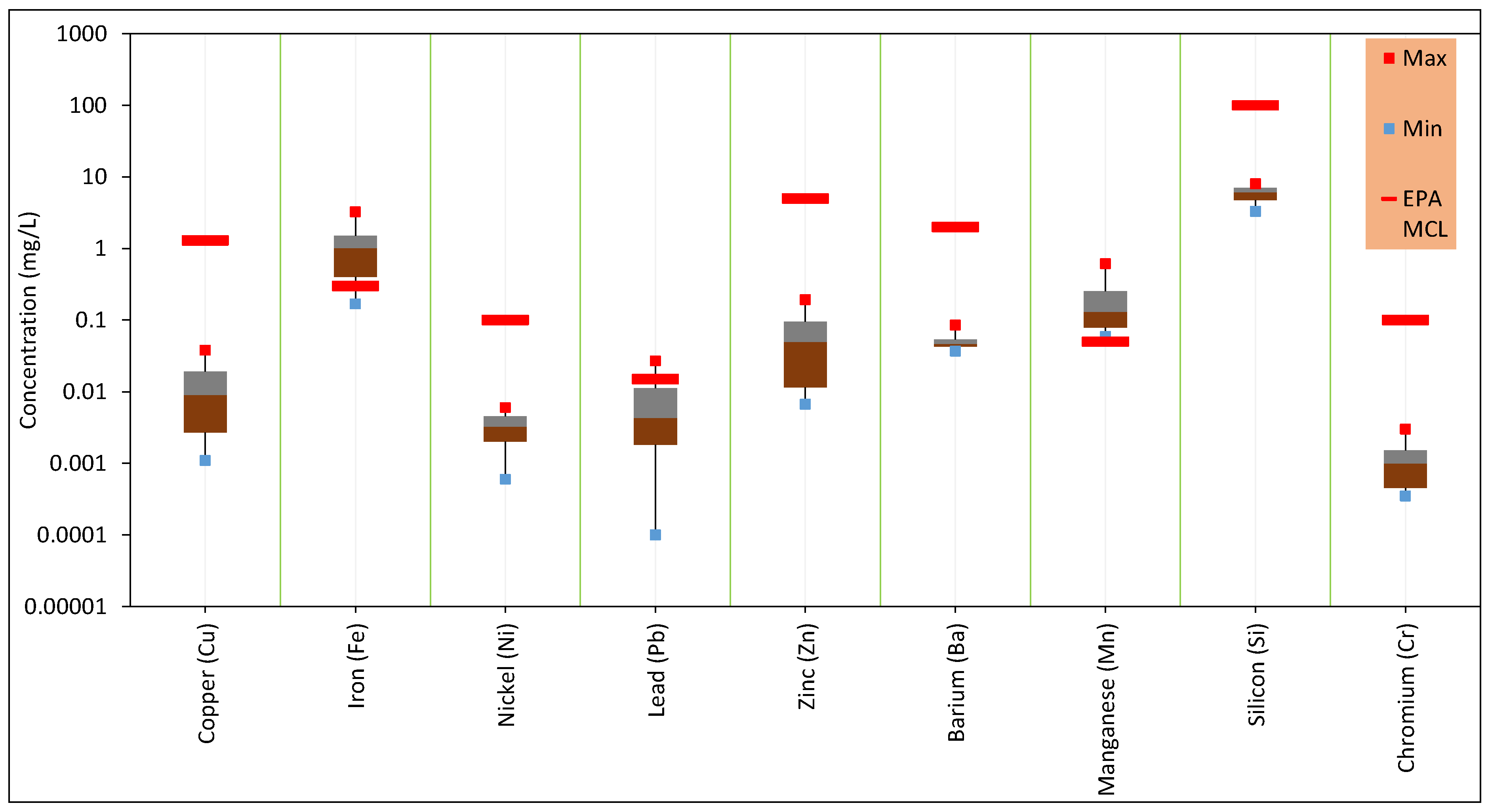
3.1. Water Quality Analysis

A total of eight storm events (i.e., twenty-four (24) water samples were collected, one during each stage) were analyzed, of which 37.5% were taken in 2020 during the imposition of the COVID-19 restrictions, while the rest were collected in 2021 (25%) and 2022 (37.5%). Even though the number of storms was high enough to develop the analyses, the authors recommend including automatic sampling, if possible, to minimize errors.
All water quality parameters (i.e., pH and conductivity), along with streamflow, ADD, and the total number of vehicles, are detailed in Table 2. Stormwater conductivity ranged from 381 to 1266 μmhos, while ADD was documented to be between 1 and 15 days. Moreover, the streamflow’s pH ranged between 4.6 and 8.6, though typical pH values in surface waters (not stormwater) in Denver are generally basic (between 8.5 and 9.2) [47]. However, most pH values in LG fell within the acceptable range (6.5 to 9) for Colorado Surface Water Quality Standards [16]. Nevertheless, April flows showed acidic conditions (pH between 4 and 5), which could either be due to the nitric acid naturally contained in precipitation for a particular storm [48] or possibly traffic-related pollution [49]. Acidic water has a negative effect on aquatic ecosystems, leading to a decrease in the number of plankton and benthic invertebrate species and the reproductive failure of acid-sensitive species of amphibians (e.g., leopard frogs and salamanders) [50], while also altering chemical conditions such that they become toxic to fish and other aquatic animals [51]. Additionally, drinking acidic water might make a person sick, damage certain tissues, and may even result in fatality [52]. Therefore, the regular monitoring of pH is highly recommended for LG and Denver’s urban watersheds with streams. Cement porous pavements (CPP) may be used to increase the pH in stormwater in Denver [53], though other methods could be tested as well; for example, Kazemi and Hill [54] used permeable basalt-based aggregates to increase the pH in stormwater near Athelstone, South Australia.
The MCLs set by the EPA for drinking water are often used as a metric of anthropogenic impacts on natural aquatic systems (e.g., [45]). Based on the literature [8,11,55,56], all selected metals (Fe, Mn, Pb, Zn, Cu, Ba, Ni, Cr) except for Si are traffic-related and thus are relevant for this analysis. However, Table 3 and Figure 2 show that Ni, Cr, and Zn generally have very low concentrations, often approaching the detection limit or perhaps representing background concentrations. Cu and Ba display concentrations well above the detection limit but always an order of magnitude below the MCL. Thus, our analysis of metal pollution will primarily focus on Fe, Mn, and Pb. However, the analysis of Cu, Ba, and Zn can be useful for some analyses (i.e., assessing whether traffic is a primary source of pollution) because they have concentrations that vary substantially between storms and that are well above the analytical detection limit. This approach is supported by Wang et al. [38] and Müller et al. [57], who concluded that metals such as Ba, Cu, Fe, Mn, Pb, and Zn can originate from vehicles. Before analyzing the potential traffic source, however, a traditional water quality analysis is provided.
Fe and Mn exceeded regulated standards in every sampled storm event, showing high variability within the three-year sampling period, with maximum values of 3.2 and 0.6 mg/L, respectively. A Fe concentration of 3.2 mg/L in stormwater is considered highly polluted, because the MCL for this metal is only 0.3 mg/L. Similarly, Pb exceeded legal concentration limits on five occasions (three events), peaking at nearly 0.027 mg/L, which is higher than the regulated limit of 0.015 (see Figure 2). These results agree with the findings by Li et al. [58], who investigated Mn, Pb, and Fe in Beijing (China) and reported that these metals also exceeded local water quality standards.
Previous studies developed in different cities around the world, in contrast to what was obtained in this investigation, are listed in Table 4. The mean Fe, Mn, Pb, and Zn concentrations in Denver are 3.590 mg/L, 0.268 mg/L, 0.056 mg/L, and 0.761 mg/L, respectively. Generally speaking, the mean concentrations determined in this study are greater than the concentrations obtained in Sweden [59] and Japan [60], likely due to a high reliance on private vehicles instead of public transportation or the different regulatory framework governing traffic vehicle emissions between the US and these countries. However, climate might play a crucial role, as Stockholm (Sweden) and Shiga (Japan) receive around 550 [61] and 1590 mm [62] of annual precipitation, respectively, which is higher than semiarid Denver, which receives only around 363 mm/year, and a significant portion of it falls as snow during winter months [34]. Experiencing rainfall more often in a given city means streets being cleaned regularly, resulting in cleaner stormwater.
In contrast, the pollutant concentrations obtained in this study are lower than those reported in Australia [63], United States (Texas [64] and California [65]), China [56], Peru [66], and France [11] (see Table 4). Many factors can explain these differences, but considering the city of Arequipa in Peru as an example, with highly polluted stormwater samples [66], a possible explanation is the difference in climate, as this South American city receives less than 144 mm/year of rainfall [67], meaning more pollutants accumulating on streets and fewer washing events. Similarly, the types of vehicles that circulate in Arequipa are characterized as being old and in poor repair [66], which can lead to greater leakage of contaminants. Finally, the land use characteristics in the Peruvian study site are composed mostly of cement, with a complete absence of green areas, located in a part of the city characterized by heavy traffic flow (downtown Arequipa). In contrast, LG has 363 mm/year of precipitation [34], with relatively newer cars or better maintained cars due to stricter environmental regulations, lower vehicular traffic intensity, and green and natural areas account for 4% and 18% of the area, respectively.
Table 4. Metal concentrations in urban stormwater from the literature (mg/L).
ReferenceCityFeMnPbZn
This studyDenver, CO, USA1.890.290.0150.111
[59]Stockholm, Sweden0.040.020.000140.100
[60]Shiga, Japan1.570.050.0140.502
[56]Chaoyang, China 0.1001.000
[64]Austin, TX, USA3.54 0.0990.237
[63]Nerang, Australia5.500.080.0300.200
[66]Arequipa, Peru9.000.900.0115.000
[11]Paris, France 0.0250.260
[68]Mount Rainier, MD, USA 0.1900.001
[65]Multiple cities in CA, USA 0.0800.203
Average 3.5900.2680.0560.761

3.2. Pollutant Mass Loads: General Analysis

Mass load distributions, using flow and concentration data in Table 2 and Table 3, are illustrated in Figure 3. Fe, Mn, and Pb (the pollutants that were found at levels above the EPA standards) showed a wide range of loading rates, with average loading rates of 2699, 464, and 19 mg/s, respectively. Si is not generally considered a traffic pollutant, as previously mentioned, and its high concentrations are expected based on the typically high concentrations of silica in Denver-area sediments [40].
Moreover, based on our sampled storm events and considering a documented average summer stormflow duration of 126 min for the three years under study (all based on Table 3, excluding the first unusually longer event), and an average of 22 summer storm events (May through August between 2020 and 2022) per year in LG (having a drainage area of 3354 ha), the watershed is estimated to have 0.4489, 0.0772, and 0.0032 MT, or 1.34 × 10⁻⁴, 2.3 × 10⁻⁵, and 1.0 × 10⁻⁶ MT/ha of Fe, Mn, and Pb, respectively, being released directly into the South Platte River from the watershed every year.
Huber and Helmreich [37] estimated the traffic-related emissions in Germany for seven different sources (tire wear, brake lining wear, roadway abrasion, weights for tire balance, guardrails, lampposts/signs, and de-icing salts), and determined a level of 0.003 MT/year-ha for Pb. Their results were much higher than those obtained in this study, most likely because the authors estimated total annual pollution considering all highways nationwide. In Cranston (USA), Hoffman et al. [69] reported levels of 0.28, 0.054, and 0.14 Mg/year-ha for Fe, Mn, and Pb, respectively, demonstrating higher annual pollution levels than those obtained in this study, most likely because the authors sampled stormwater near a busy highway, even though their drainage area was only 44 ha. Moreover, the previously mentioned study by Martínez et al. [66] in Arequipa (Peru) also reported that Fe, Mn, and Pb concentrations (and loads) were above those set out by local environmental regulations, though the authors did not provide enough information to estimate annual pollution loads.

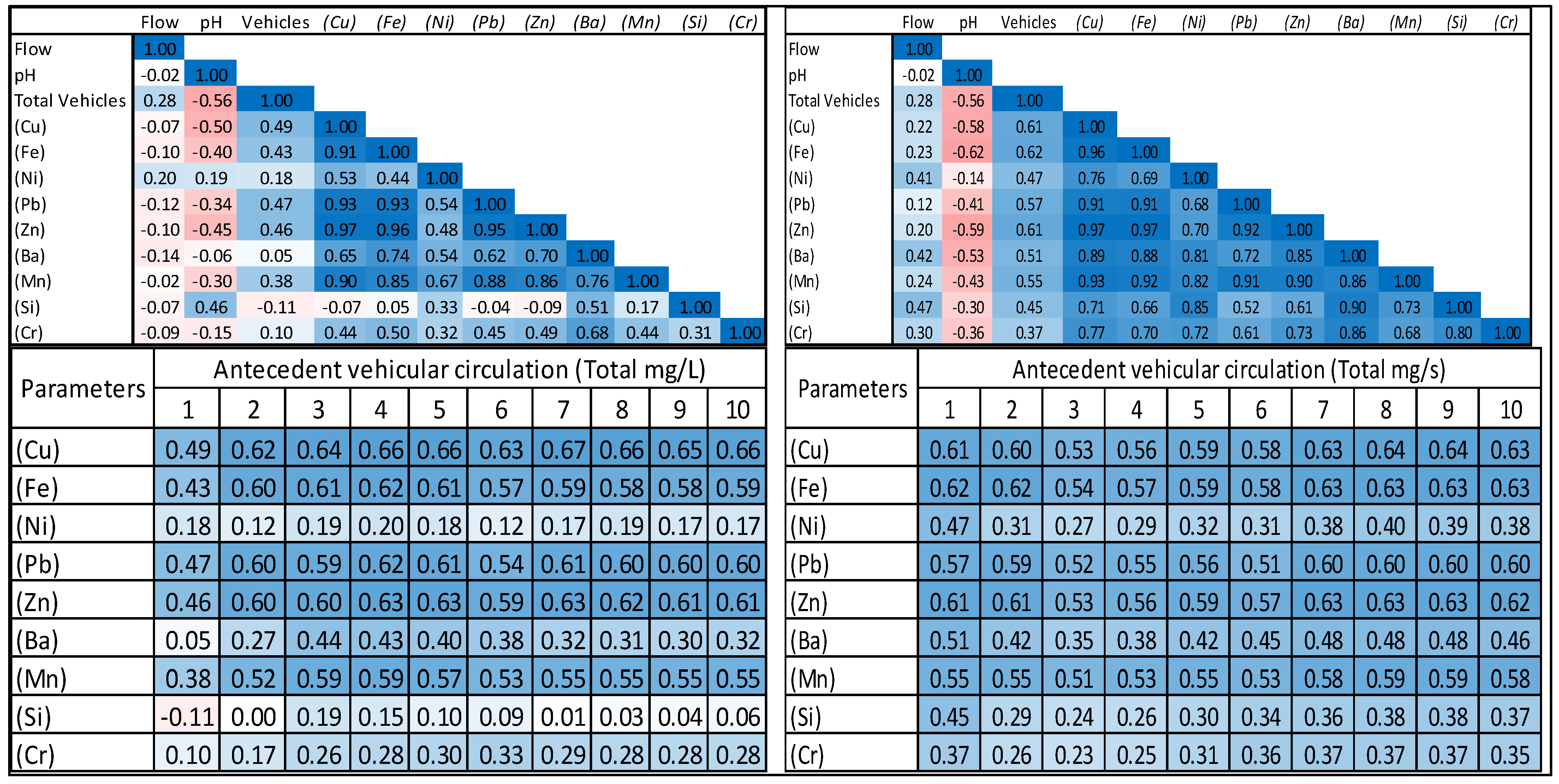
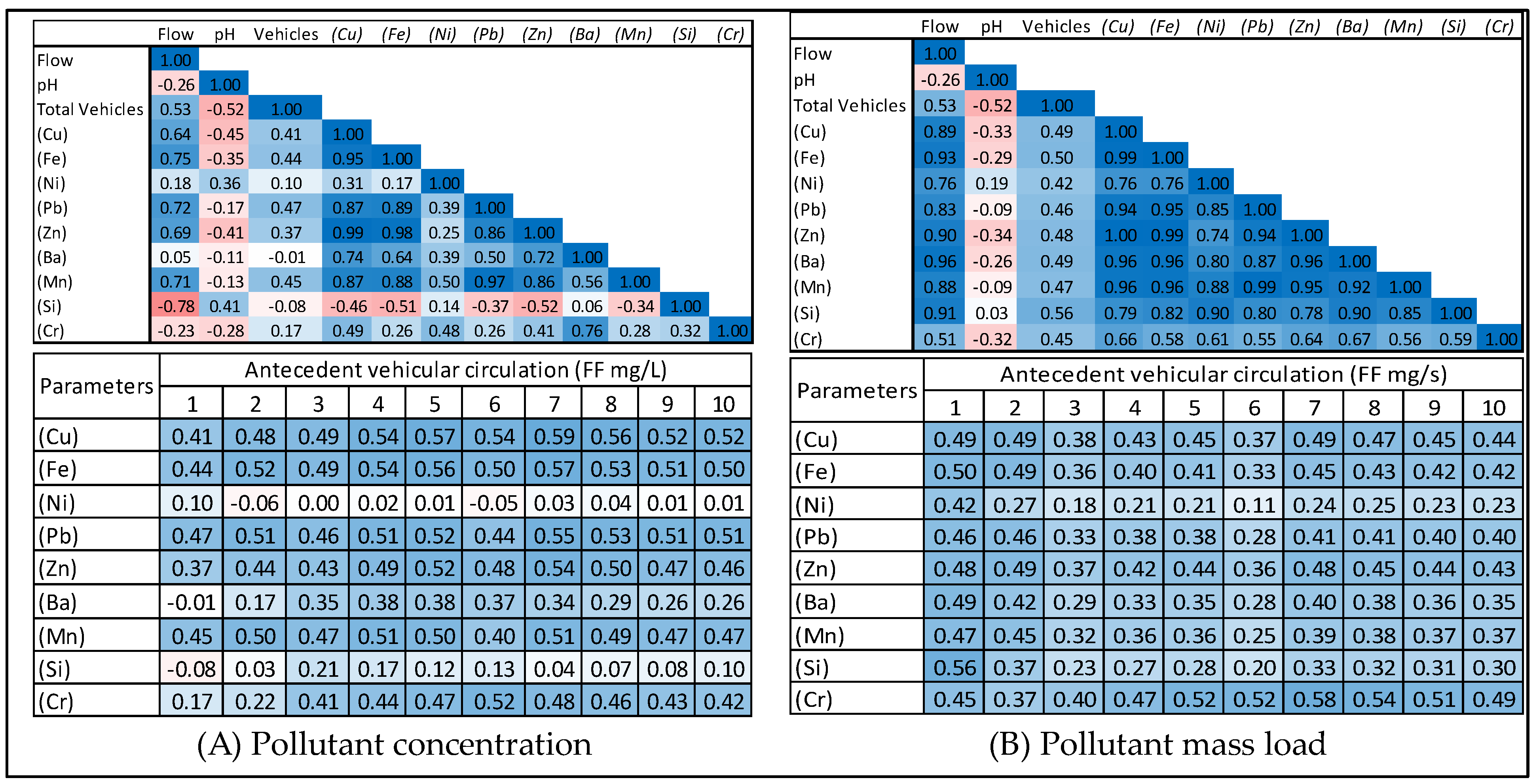
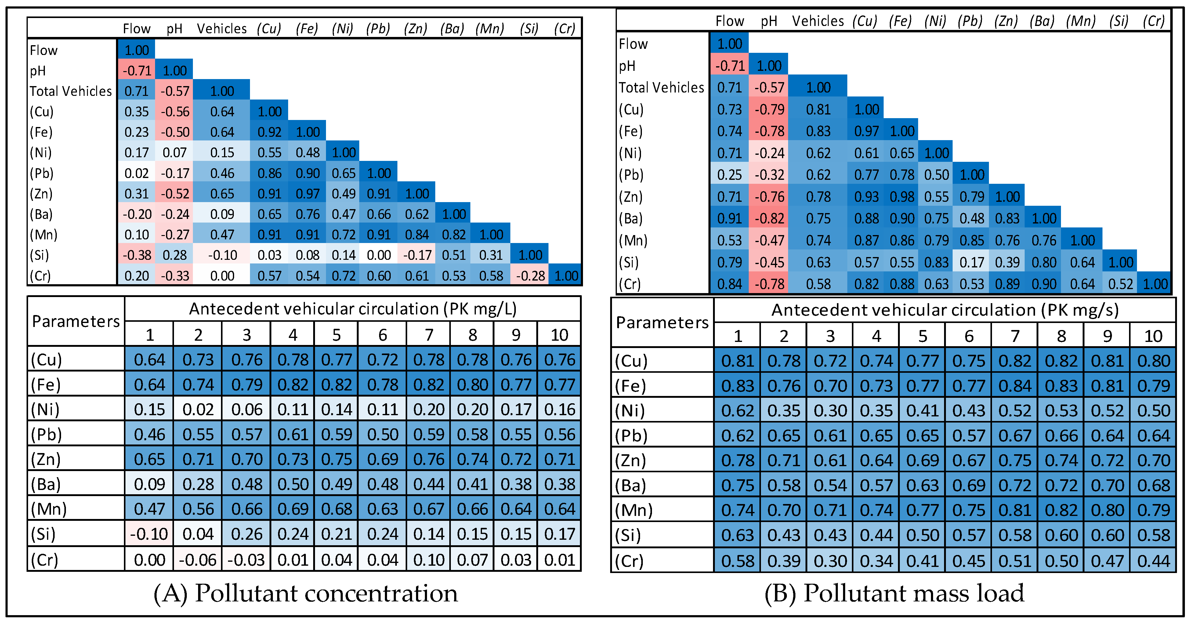
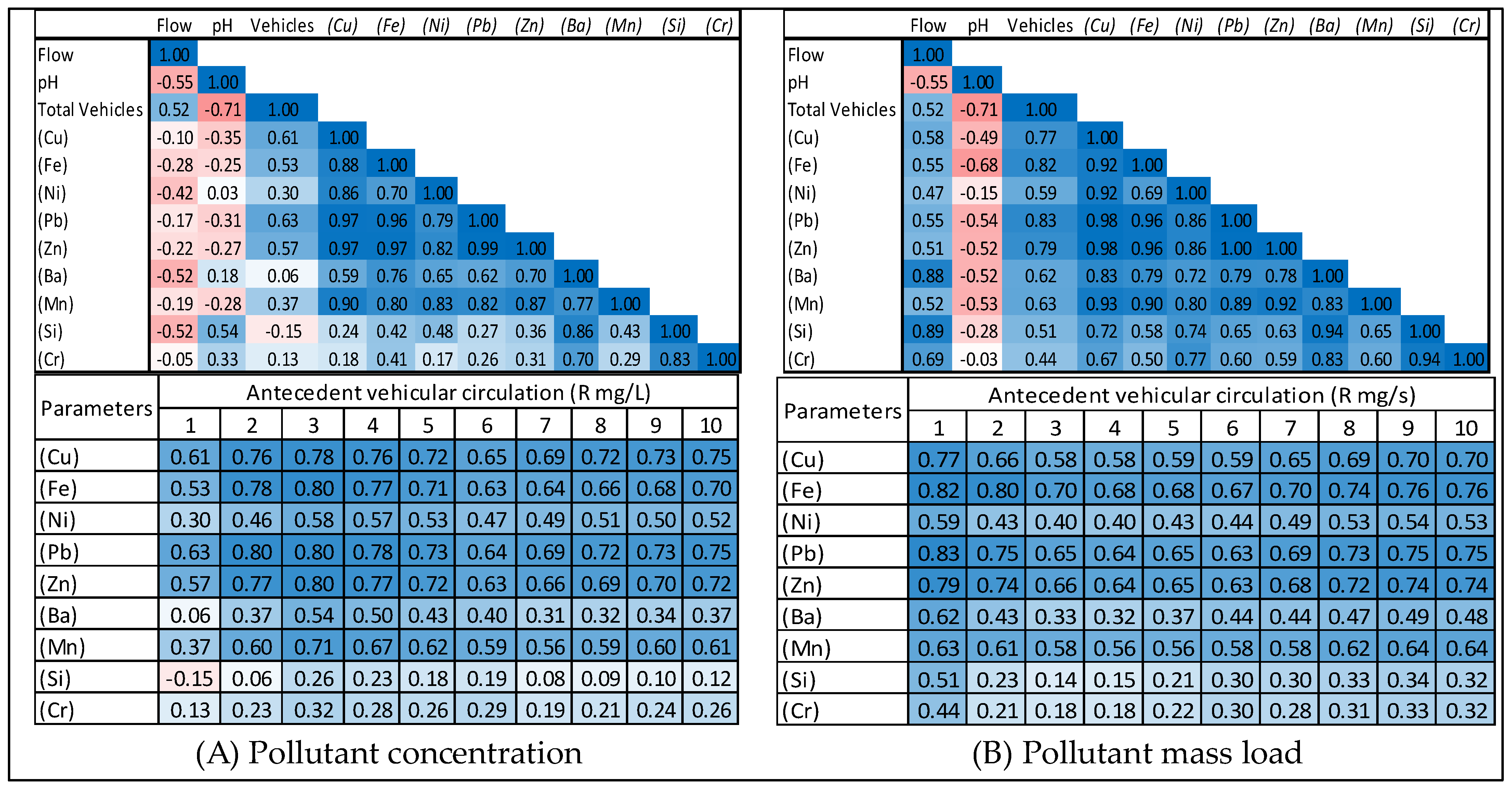
3.3. General Relationships Between Water Quality Variables

Using the data in Table 3, a correlation matrix was created for metal concentrations and metal mass load considering all data (top in Figure 4), and we assessed their correlation with the number of vehicles during each of the first 10 days of antecedent vehicular activity (bottom in Figure 4) to better understand the potential causal relationships. High, positive Pearson correlation coefficients were documented among all pollutants (i.e., the pollutants were all correlated with each other). The significant positive correlations (typically exceeding 0.80) among metal pollutants suggest that they probably originate from the same source of pollution, although this analysis alone cannot identify that source. As stated earlier, Cr and Ni generally displayed exceptionally low concentrations that were similar for all storms, approaching the analytical detection limit, and thus were possibly at background levels. Similarly, Si was more associated with geological sources. As such, any correlations for these pollutants, or lack thereof, are likely not useful for correlating traffic with water pollution.
Metal concentrations are weakly and positively correlated with stormflow rates, which is surprising, given that our traditional conceptual model would suggest that higher flows would dilute a fixed mass of pollutants on impervious surfaces, resulting in lower concentrations (or an inverse correlation). Flow is more strongly and positively correlated with pollutant mass loads, largely because the total flow is used in the calculation to obtain mass loads (Equation (1)). A more detailed discussion of metal concentrations and mass loads at different hydrograph stages is presented in the next section.
Both metal concentrations and mass loads are positively correlated with the total number of vehicles associated with the storm wherein the samples were collected. In addition, the correlations between traffic volume and pollutant mass loads are stronger than between traffic volume and pollutant concentrations, as expected, for the reasons stated earlier. Indeed, Figure 4 (bottom) shows that the correlation between pollutants and antecedent traffic is strong and positive for the first 10 days prior to sampling, as discussed in a forthcoming section. ADDs greater than 10 days were not included in the analysis due to street sweeping schedules. Sweeping removes pollutants from the streets. The city of Denver sweeps regularly in residential streets twice per month, but different neighborhoods within the watershed are swept on different days. The major highways, such as Federal Blvd and US Highway 6, are not swept as often, but the schedule is not regular. Part of the watershed is in the community of Lakewood, which has street sweeping about every 10 days, but the schedule is not regular, and again different neighborhoods have different schedules. Thus, we could not directly account for street sweeping. For these reasons, a 10-day antecedent period was deemed appropriate for this analysis.
Discussions on traffic’s impact on metal concentrations and loads at the different flow stages (Ff, Pk, R), as well as the impact of traffic during and after the imposition of the COVID-19 restrictions, on metal pollution are presented in the forthcoming sections.

3.4. Stormwater Metal Pollution at Different Hydrograph Stages

Numerous studies have been performed on stormwater quality during different hydrograph stages, particularly during the first flush (Ff) stage [70,71,72]. Most studies stated that maximum pollutant concentrations occur either at the Ff or peak (Pk) stages, with the majority of them concluding that the largest loads typically occur during the Ff (e.g., [68,73]). However, the results from these papers regarding pollutant loads for various stages are not conclusive. For example, Flint and Davis [68] evaluated stormwater quality in Mount Rainier (Maryland, USA) and stated that only about 33% of storms exhibited the highest pollutant load during Ff. Shumi et al. [73] analyzed pollutants including Pb and Fe in Chongqing (China), concluding that there was no Ff effect in the study area. Few studies have reported loadings during the recession period. Our research showed that maximum pollutant concentration often occurs during the Pk (39%) and recession (R, 57%) stages, with fewer (4%) storms exhibiting the highest pollutant concentrations or loads during Ff (see Table 3).
The results from Table 3 show an irregular pattern of concentration among all pollutants (and other measured variables) at various stages within storm events. Those pollutant concentration variations within a given storm agree with the findings by Shorshani et al. [11], who studied urban stormwater quality near Paris (France). In our research, for example, on 11 April 2020, similar concentrations were observed during all stages (Ff, R, and Pk) for all metals. However, on 15 May 2020, concentrations during the storm were very different for each stage and for each metal; for this particular storm, Fe concentrations gradually increased as the storm occurred. In short, there was no consistent trend of metals during the different flow stages. For example, Fe (a metal of concern) had peak values during the R stage in six out of eight events, while Mn displayed a peak concentration during R in four out of eight events.
Moreover, the correlation matrix between metal concentrations and related variables during various stages yields interesting results (Figure 5, Figure 6 and Figure 7, upper left). Figure 5 (top left) shows that for correlations during the Ff stage for all storms, metal concentrations are positively correlated with the flow (usually between 0.64 and 0.75), except for Si (−0.78) and Cr (−0.23), which as stated previously are probably not relevant due to not being related to traffic or being near background levels. That is, higher first-flush flows tend to have higher concentrations. Peak flows (Figure 6, upper left) also exhibit moderate positive correlations with metal concentrations, although not as high as during the first flush, at generally between 0.10 and 0.35, except for Ba (−0.20) and Si (−0.38). Conversely, concentrations are weakly and mostly negatively correlated with recession flow (Figure 7, upper left) for all the pollutants.
Interestingly, mass loads are positively correlated with flow at all stages of the hydrograph (Figure 5, Figure 6 and Figure 7, upper right). Flow is used to calculate mass loads (Equation (1)), providing a partial explanation for this correlation, although concentrations are also used in the calculation, so in general we do not necessarily expect a strong positive correlation between mass load and flow. Mass loads also show higher positive correlations with the flow during Ff (0.51 to 0.96, with Si at 0.91) than at the other stages. However, the Ff correlation is only slightly higher than during Pk flow (0.25 to 0.91, with Si at 0.79) or R flow (0.51 to 0.88 with Ni at 0.47, Si at 0.89, Ba at 0.88 although as discussed before, Ni and Ba are likely not relevant). So, Si in all cases is highly correlated with flow, which generally results in higher sediment loads, as Si is typically associated with all sediment particles in the Rocky Mountain region [40].
It is interesting that within each hydrograph stage, metal concentrations are linked to flow, but generally not as high as Si (which is likely sourced from sediment), which suggests that metal loading is not primarily from suspended sediments (and we do not expect this in an urban area). One potential explanation is that, for this small urban watershed, higher flows allow more runoff areas and pathways to be connected. That is, additional areas of the watershed become part of the runoff at higher flows, including additional metal sources and less polluted water infiltrating these previously excluded impervious surfaces. Additionally, a significant portion of the watershed is covered by natural areas, as explained previously. Finally, there could be a link between Si loads and construction activities within this urban watershed, but more research would be necessary to confirm this.
In terms of the impact of traffic on metal concentrations and loads at different hydrograph stages, all stages generally show positive correlations between 0.40 and 0.80, meaning the more vehicles there are circulating, the higher the concentration of most pollutants of concern (i.e., Fe, Mn, and Pb) and others like Zn, with the best correlations occurring during Pk (see Figure 5, Figure 6 and Figure 7, upper left), as discussed later. Correlations were even stronger when considering vehicular circulation and mass loads (see Figure 5, Figure 6 and Figure 7, upper right). The analyses shown in Figure 5, Figure 6 and Figure 7 (upper left and upper right) were performed considering the vehicles that circulated during the day of sampling (until the time of sampling), i.e., during the first antecedent vehicular circulation day. Moreover, there was a strong correlation between metal concentration and mass load and vehicular activity for all ten antecedent circulation days (see Figure 5, Figure 6 and Figure 7, lower right and lower left), suggesting an acute effect of vehicular traffic on metallic pollution. The substantial contribution of vehicular traffic to metal pollution in stormwater, especially in the initial phases of runoff events, is highlighted by the significant correlations observed in this investigation. Typically, correlations weaken with increasing antecedent vehicular circulation days, suggesting a dilution or attenuation effect from other sources over time. The reasons for these high correlations over time are unknown.
In the correlation matrix, the Total Vehicles category exhibits positive correlations with the majority of metal contaminants throughout all hydrograph stages (see Figure 5, Figure 6 and Figure 7). Correlations between total vehicles and pollutant concentrations are generally weak for Ff (0.47) and moderate for R (0.06 to 0.63). The correlations are stronger during Pk conditions (between 0.3 and 0.65), with Cu, Fe, and Pb particularly impacted by vehicle numbers. Stronger correlations for these pollutants are logical, since these metals are associated with traffic. Other studied variables such as flow (except the first flush, described above) and pH show weaker correlations with pollutants at the different stages, indicating a less direct influence compared to vehicle numbers.
We believe that mass loads are a more important metric for urban stream pollution because they are less subject to storm size and dilution, and theoretically more related to the source of pollution. In addition, mass loading is the most common way to regulate stream pollution (i.e., pollutant maximum daily load, TMDLs), even though MCLs are often used to indicate the severity of pollution. Correlations between pollutant mass loads and traffic revealed a similar trend as for pollutant concentrations, but stronger (see Figure 4, Figure 5, Figure 6 and Figure 7). During Ff (Figure 5), the correlations between the number of vehicles and pollutants are generally lower than those during Pk and R (i.e., 0.42 to 0.56), and are remarkably similar for all pollutants, at about 0.40. During the Pk stage (Figure 6), these correlations are stronger (0.58 to 0.81), where correlations for all metals except Si (0.63) are again remarkably similar to each other. During the R stage (Figure 7), correlations are again stronger (i.e., 0.44 to 0.83). Overall, the correlations between mass loading and traffic suggest that traffic is likely a leading cause of metal pollution in our urban watershed during storms.
Increased traffic intensity leads to more pollutants, and the cumulative effect of this pollution may result in elevated contaminant concentrations and loads in stormwater runoff from high-traffic zones [74]. Thus, high-traffic areas experience more frequent and intense abrasion of road surfaces, releasing metal pollutants, as investigated by Shajib et al. [56]. Apeagyei et al. [75] looked at how heavy metals were distributed in road dust in both urban and rural parts of Massachusetts (USA), concluding that road dust is a significant contributor to pollution in stormwater runoff. Wang et al. [38] quantified the metals emitted from vehicles on an urban highway in Toronto (Canada) and found that Fe emissions are up to three times higher at highway sites due to the presence of more vehicles circulating. Similarly, Shorshani et al. [11] simulated the integrated traffic, air, and stormwater quality in Grigny (France), concluding that the contribution of local traffic to stormwater contamination is significant for Pb and Zn, agreeing with our findings. Moreover, the exact impact on Swedish stormwater quality due to metals from traffic (particularly Zn) was described by Müller et al. [57], while Czemiel Berndtsson [30] studied stormflow in Trelleborg (Sweden) and concluded that heavy metal concentrations were directly correlated with the number of traffic vehicles. Additionally, Dang et al. [76] studied pollutant concentration during stormwater runoff events in Nantes (France) and showed that wet weather events occurring during high-traffic hours contribute to elevated levels of stormwater pollutants such as Pb, Ni, Zn, and Cu. All those investigations agree with our findings, i.e., the more vehicles there are circulating, the higher the pollution in stormwater.

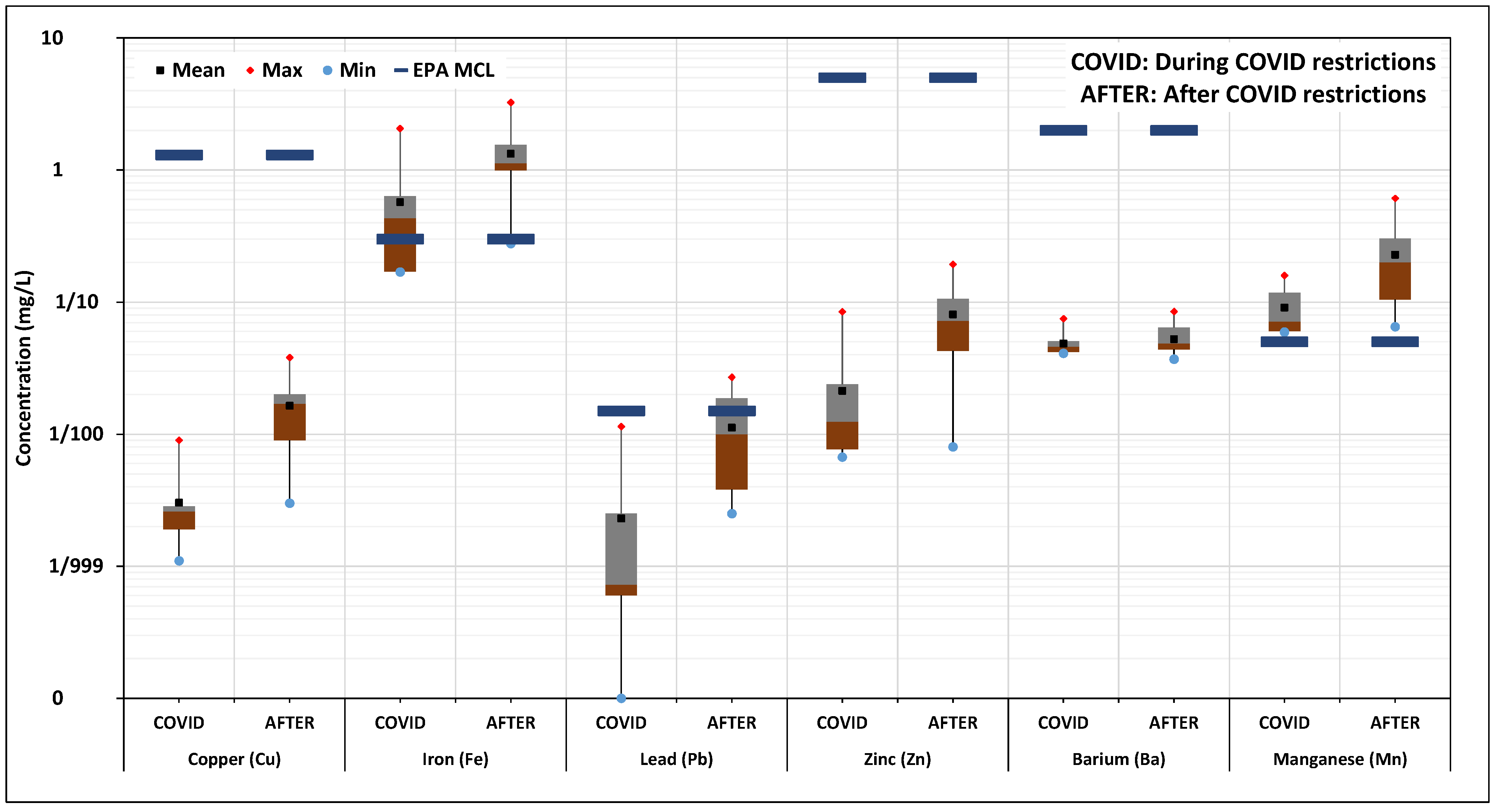
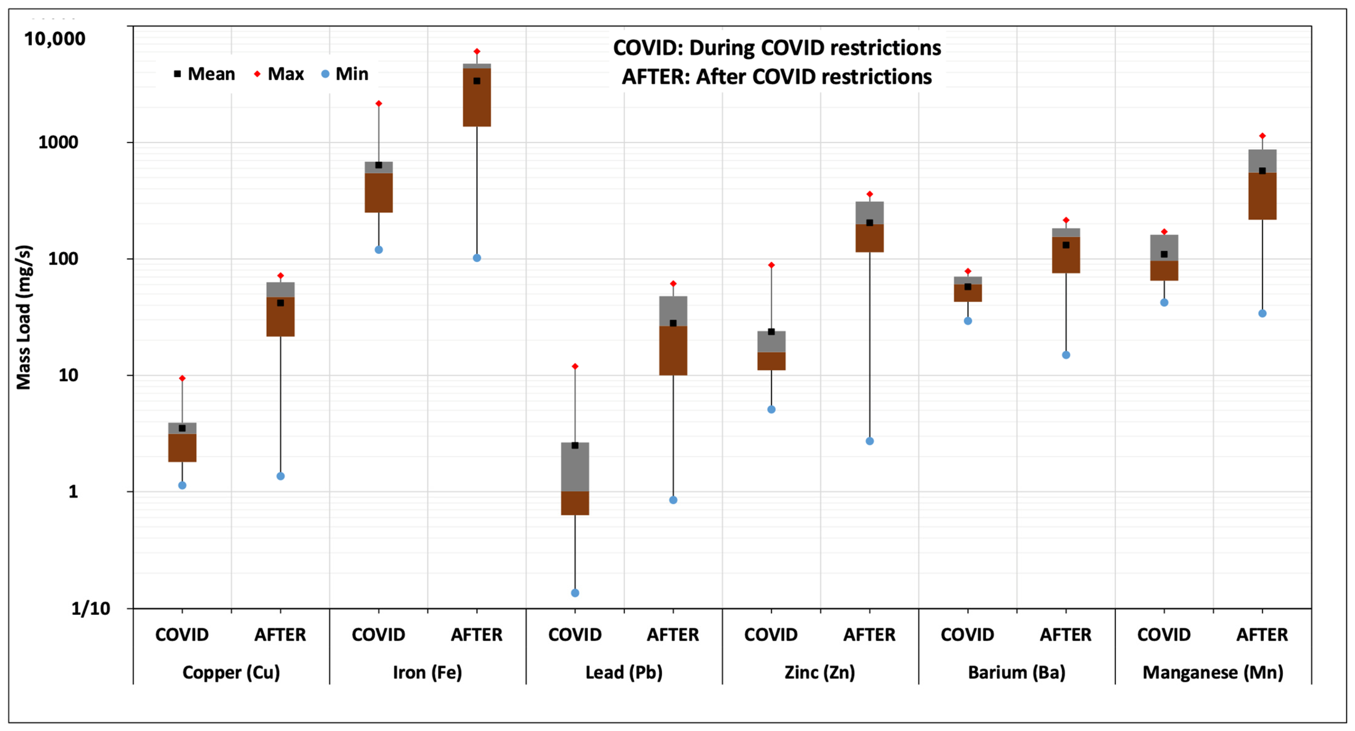
3.5. Effects of COVID-19 Restrictions on Stormwater Pollution

As discussed previously, we believe that mass loads are a better metric to evaluate sources, and these are presented in Figure 3. Figure 8 shows mass loads during the enforcement of the COVID-19 restrictions (labeled “Covid”) and after restrictions were lifted (labeled “After”). As discussed previously, the more useful traffic-related metals to consider are Fe, Pb, Mn, Zn, Cu, and Ba. Ni and Cr had very low, nearly constant concentrations (see Figure A1) near the analytical detection limits, suggesting these may be background concentrations that are likely not related to any transient source, such as traffic. Cu, Ba, and Zn, while exhibiting low concentrations, are included because they are linked to traffic (as described earlier) and have variable concentrations well above background that could be linked to a source.
There was an increase in vehicular activity after the COVID-19 restrictions were lifted (from an average of 10,409 to 63,224 vehicles per day in LG, respectively), calculated based on data from Table 2. Even though a scientific analysis of how the COVID-19 pandemic affected vehicular activity in Colorado has not been performed previously, Harantová et al. [77] estimated the effect of COVID-19 on traffic flow characteristics in Slovakia and reported a 70% decrease in traffic during 2020. Moreover, Haghnazar et al. [78] analyzed Pb and Zn levels in stormwater in the urban Zarjoub River (Iran) and found that during the enforcement of COVID-19 restrictions, stormwater pollution decreased by 30%. Similarly, Chakraborty et al. [79] also examined river water quality behavior in Damodar (India) and found that 100% of water samples were polluted after the COVID-19 restrictions were lifted, while only 9% of the samples collected during the imposition of restrictions were contaminated.
As illustrated in Figure 8, the mass load is significantly lower for most metals during the enforcement of the COVID-19 restrictions compared to after restrictions were lifted. For instance, Fe shows a median load of about 100 mg/s during the restrictions, increasing to approximately 1000 mg/s post-restrictions. These results indicate that higher vehicle counts lead to substantially increased metal pollutant loads in stormwater runoff. More pollutant mass loads were documented when more vehicles were circulating, i.e., after the COVID-19 restrictions were lifted (see Figure 8). In general, the results support previous research that has already been mentioned, suggesting that there is a correlation between increased metal levels in urban runoff in LG and increased traffic intensity in Denver prior to wet weather events.
Interestingly, a more important result might be that fewer vehicles on the road lowered the mass load of metal contaminants in stormwater runoff, suggesting that future sustainable urban development typically intended to reduce traffic should also improve urban water quality. Moreover, public habits that are becoming more common and result in less vehicular transportation (e.g., remote work, remote education, and online shopping) can also have a positive impact on stormwater quality in urban aquatic ecosystems. Similarly, stormwater management practices are needed to reduce the dangers that vehicle pollution poses to people’s health and the environment, especially in heavily populated cities. For example, elevated concentrations of metals in stormwater can be reduced by oxidation ponds and wetlands [80], as well as infiltration-based technologies (e.g., [81,82]) and green infrastructure. For example, Walker and Hurl [83] investigated the efficiency of a wetland in stormwater treatment, concluding that the concentration of metals such as Zn, Pb, and Cu can be decreased by 57%, 71%, and 48%, respectively, through the structure. Similarly, Jacklin et al. [84] were able to remove most detectable metals using green infrastructure approaches. The current research suggests studying the long term trends of stormwater pollution after the COVID-19 pandemic and developing predictive models for simulating the impact of future traffic scenarios providing in-depth insights for both policy makers and urban planners. Following the discussion of findings in this research, it is also very important to acknowledge the limitations of this study, namely the traffic data collection process, in which we could have measured the data more accurately via physical surveys during the period of COVID-19 restrictions, and the results could also have been compared with the data collected from OTIS. Similarly, the water samples could also have been collected for more events at different times during the period of the COVID-19 restrictions, which could have increased the sample size, allowing for a more detailed comprehensive study. Future research should also consider the changes in land use patterns in relation to stormwater quality, which will be beneficial for understanding of urban pollution dynamics.

3.6. Innovative Points and Limitations of This Study

The innovative points of this study include highlighting the impact of traffic vehicles on heavy metal concentration, specifically the significant correlation between vehicular circulation and stormwater pollutants during and after the enforcement of COVID-19 restrictions. Moreover, the results from this investigation provide valuable insights for urban stormwater pollution management, clearly suggesting that (1) even in a drainage area mostly occupied by residential land use (i.e., low traffic) with nearly 25% of the watershed covered by green and natural areas, urban stormwater quality can contain dangerous pollutants in concentrations above environmental standards, representing a risk to aquatic ecosystems, and (2) efforts should be focused not only on stormwater treatment practices but also on finding ways to decrease vehicular circulation, as previously discussed.
However, this investigation also involved some relevant limitations, such as the usage of a smaller dataset and limited observation times, which may not have captured the variability in pollutant concentrations. Therefore, future research should include continuous sampling to provide a better idea of how pollutant concentrations and mass loads change during storms. Even though such an approach is more expensive, it might be an important component in future investigations. Similarly, this study did not consider how land use and other variables such as rainfall intensity, wind speed, and other climatic variables affect stormwater pollution.

4. Conclusions and Recommendations

This study, conducted on the Lakewood Gulch urban watershed in Denver, provides several key insights into the impact of vehicular traffic on stormwater metal pollution. Stormwater consistently exceeded the maximum contaminant levels (MCLs) for Fe and Mn, though Pb was occasionally above the drinking water standards. Using historical local storm intensity and volume data, annual Fe, Mn, and Pb pollution loads were estimated to be 1.34 × 10⁻⁴, 2.3 × 10⁻⁵, and 1.0 × 10⁻⁶ MT/year-ha, respectively, with these values being considered about average when compared to research conducted elsewhere and being explained by the local climate and development level.
While examining metal pollution at different hydrograph stages, it was evident that there was an increase in pollutant concentration and mass loads during peak flow conditions, agreeing with findings from research developed elsewhere. The first flush effect was not as profound as expected, which has also recently been noted by several papers for stormwater pollutants in general.
Importantly, our results suggest that stormwater pollution increased when more vehicles were circulating. Moreover, the COVID-19 pandemic offered a unique opportunity to evaluate the effects of historically low traffic activity in Denver, and when comparing stormwater quality during and after the enforcement of COVID-19 restrictions, it was clear that less pollution occurred during the restrictions. Those results suggest that future sustainable urban development typically intended to reduce traffic would also improve urban water quality, providing additional motivation for reducing traffic during urban development or re-development. Similarly, public habits that are becoming more common and can result in less vehicular transportation (e.g., remote work, remote education, and online shopping) can also have a positive impact on stormwater quality in urban areas. Finally, stormwater management practices are needed to reduce the dangers that vehicle pollution poses to people’s health and the environment, especially in heavily populated cities.

Author Contributions

Conceptualization, K.A.S. and P.G.-C.; methodology, P.G.-C. and J.E.M.; formal analysis, K.A.S. and P.G.-C.; investigation, J.E.M.; writing—original draft preparation, K.A.S. and P.G.-C.; writing—review and editing, K.A.S. and J.E.M.; supervision, J.E.M. and P.G.-C. All authors have read and agreed to the published version of the manuscript.

Funding

This work was partially supported by NSF RAPID, through the NSF Hydrology Program, (NSF 2031614), and was also partially supported by the National Science Foundation-funded Engineering Research Center (ERC) for Reinventing the Nation’s Urban Water Infrastructure (ReNUWIt) (NSF EEC-1028968).

Data Availability Statement

Data is available upon request.

Acknowledgments

The authors express their gratitude for the support from the National Science Foundation. Additionally, the authors thank the Colorado School of Mines graduate and undergraduate students that helped with sample collection during storms at the study site.

Conflicts of Interest

The authors declare no conflicts of interest.

Appendix A

Figure A1. Statistical distribution of pollutant concentrations during and after the imposition of COVID-19 restrictions (blue lines indicate the MCL).
Urbansci 09 00081 g0a1

References

  1. Haque, S.E. Urban Water Pollution by Heavy Metals, Microplastics, and Organic Contaminants, 1st ed.; Elsevier Inc.: Philadelphia, PA, USA, 2022; Volume 6, ISBN 9780323918381. [Google Scholar]
  2. Song, Y.; Song, X.; Shao, G. Response of Water Quality to Landscape Patterns in an Urbanized Watershed in Hangzhou, China. Sustainability 2020, 12, 5500. [Google Scholar] [CrossRef]
  3. Sun, Y.; Guo, Q.; Liu, J.; Wang, R. Scale Effects on Spatially Varying Relationships between Urban Landscape Patterns and Water Quality. Environ. Manag. 2014, 54, 272–287. [Google Scholar] [CrossRef] [PubMed]
  4. Chowdhury, A.; Egodawatta, P.; McGree, J. Pattern-Based Assessment of the Influence of Catchment Characteristics on Urban Stormwater Quality. Water Sci. Technol. 2024, 90, 2441–2455. [Google Scholar] [CrossRef]
  5. Khatri, N.; Tyagi, S. Influences of Natural and Anthropogenic Factors on Surface and Groundwater Quality in Rural and Urban Areas. Front. Life Sci. 2015, 8, 23–39. [Google Scholar] [CrossRef]
  6. Rathi, B.S.; Kumar, P.S.; Vo, D.V.N. Critical Review on Hazardous Pollutants in Water Environment: Occurrence, Monitoring, Fate, Removal Technologies and Risk Assessment. Sci. Total Environ. 2021, 797, 149134. [Google Scholar] [CrossRef]
  7. Gabr, M.E.; El Shorbagy, A.M.; Faheem, H.B. Assessment of Stormwater Quality in the Context of Traffic Congestion: A Case Study in Egypt. Sustainability 2023, 15, 13927. [Google Scholar] [CrossRef]
  8. Liu, A.; Ma, Y.; Gunawardena, J.M.A.; Egodawatta, P.; Ayoko, G.A.; Goonetilleke, A. Heavy Metals Transport Pathways: The Importance of Atmospheric Pollution Contributing to Stormwater Pollution. Ecotoxicol. Environ. Saf. 2018, 164, 696–703. [Google Scholar] [CrossRef]
  9. Müller, A.; Österlund, H.; Marsalek, J.; Viklander, M. The Pollution Conveyed by Urban Runoff: A Review of Sources. Sci. Total Environ. 2020, 709, 136125. [Google Scholar] [CrossRef]
  10. Markiewicz, A.; Björklund, K.; Eriksson, E.; Kalmykova, Y.; Strömvall, A.M.; Siopi, A. Emissions of Organic Pollutants from Traffic and Roads: Priority Pollutants Selection and Substance Flow Analysis. Sci. Total Environ. 2017, 580, 1162–1174. [Google Scholar] [CrossRef]
  11. Fallah Shorshani, M.; Bonhomme, C.; Petrucci, G.; André, M.; Seigneur, C. Road Traffic Impact on Urban Water Quality: A Step towards Integrated Traffic, Air and Stormwater Modelling. Environ. Sci. Pollut. Res. 2014, 21, 5297–5310. [Google Scholar] [CrossRef]
  12. Teixidó, M.; Schmidlin, D.; Xu, J.; Scheiber, L.; Chesa, M.J.; Vázquez-Suñé, E. Contaminants in Urban Stormwater: Barcelona Case Study. Adv. Geosci. 2023, 59, 69–76. [Google Scholar] [CrossRef]
  13. Järlskog, I.; Strömvall, A.M.; Magnusson, K.; Galfi, H.; Björklund, K.; Polukarova, M.; Garção, R.; Markiewicz, A.; Aronsson, M.; Gustafsson, M.; et al. Traffic-Related Microplastic Particles, Metals, and Organic Pollutants in an Urban Area under Reconstruction. Sci. Total Environ. 2021, 774, 145503. [Google Scholar] [CrossRef] [PubMed]
  14. Hwang, H.M.; Fiala, M.J.; Park, D.; Wade, T.L. Review of Pollutants in Urban Road Dust and Stormwater Runoff: Part 1. Heavy Metals Released from Vehicles. Int. J. Urban Sci. 2016, 20, 334–360. [Google Scholar] [CrossRef]
  15. Liu, A.; Mummullage, S.; Ma, Y.; Egodawatta, P.; Ayoko, G.A.; Goonetilleke, A. Linking Source Characterisation and Human Health Risk Assessment of Metals to Rainfall Characteristics. Environ. Pollut. 2018, 238, 866–873. [Google Scholar] [CrossRef]
  16. DDPHE Regulation NO. 38—Classifications and Numeric Standards for South Platte River Basin, Laramie River Basin, Republican River Basin, Smoky Hill River Basin. 2021; Volume 2021. Available online: https://19january2021snapshot.epa.gov/sites/static/files/2014-12/documents/cowqs-no38-2006.pdf (accessed on 1 October 2024).
  17. Gustafson, K.R.; Garcia-Chevesich, P.A.; Slinski, K.M.; Sharp, J.O.; McCray, J.E. Quantifying the Effects of Residential Infill Redevelopment on Urban Stormwater Quality in Denver, Colorado. Water 2021, 13, 988. [Google Scholar] [CrossRef]
  18. Pilone, F.G.; Garcia-Chevesich, P.A.; McCray, J.E. Urban Drool Water Quality in Denver, Colorado: Pollutant Occurrences and Sources in Dry-Weather Flows. Water 2021, 13, 3436. [Google Scholar] [CrossRef]
  19. Ali, H.; Khan, E.; Ilahi, I. Environmental Chemistry and Ecotoxicology of Hazardous Heavy Metals: Environmental Persistence, Toxicity, and Bioaccumulation. J. Chem. 2019, 2019, 6730305. [Google Scholar] [CrossRef]
  20. Ma, Y.; Liu, A.; Egodawatta, P.; McGree, J.; Goonetilleke, A. Assessment and Management of Human Health Risk from Toxic Metals and Polycyclic Aromatic Hydrocarbons in Urban Stormwater Arising from Anthropogenic Activities and Traffic Congestion. Sci. Total Environ. 2017, 579, 202–211. [Google Scholar] [CrossRef]
  21. Ghazy, M.M.E.D.; Habashy, M.M.; Nassif, M.G. The Acute Toxic Impact of Iron (Fe) and Lead (Pb) Individually and Their Mixture on Daphnia Magna (Straus, 1820). Egypt. J. Aquat. Biol. Fish. 2024, 28, 675–683. [Google Scholar] [CrossRef]
  22. Baden, S.P.; Eriksson, S.P. Role, Routes and Effects of Manganese in Crustaceans. Oceanogr. Mar. Biol. 2006, 44, 61–83. [Google Scholar] [CrossRef]
  23. Wang, X.; Liu, B.L.; Gao, X.Q.; Fang, Y.Y.; Zhang, X.H.; Cao, S.Q.; Zhao, K.F.; Wang, F. Effect of Long-Term Manganese Exposure on Oxidative Stress, Liver Damage and Apoptosis in Grouper Epinephelus moara ♀ × Epinephelus lanceolatus ♂. Front. Mar. Sci. 2022, 9, 1000282. [Google Scholar] [CrossRef]
  24. Iyare, P.U. The Effects of Manganese Exposure from Drinking Water on School-Age Children: A Systematic Review. Neurotoxicology 2019, 73, 1–7. [Google Scholar] [CrossRef] [PubMed]
  25. Ashar, Y.K.; Wulandari Panjaitan, N.; Iqbal, M.; Imron, H. Iron (Fe) Content in Community Well Water around Mabar Hilir Industrial Area Market 3 Bantenan Medan City in the Perspective of Health and Islamic. Contag. Sci. Period. J. Public Heal. Coast. Health 2023, 5, 294–301. [Google Scholar] [CrossRef]
  26. Lidman, J.; Jonsson, M.; Berglund, Å.M.M. The Effect of Lead (Pb) and Zinc (Zn) Contamination on Aquatic Insect Community Composition and Metamorphosis. Sci. Total Environ. 2020, 734, 139406. [Google Scholar] [CrossRef]
  27. Lee, J.W.; Choi, H.; Hwang, U.K.; Kang, J.C.; Kang, Y.J.; Kim, K.I.; Kim, J.H. Toxic Effects of Lead Exposure on Bioaccumulation, Oxidative Stress, Neurotoxicity, and Immune Responses in Fish: A Review. Environ. Toxicol. Pharmacol. 2019, 68, 101–108. [Google Scholar] [CrossRef]
  28. Fakhri, Y.; Saha, N.; Ghanbari, S.; Rasouli, M.; Miri, A.; Avazpour, M.; Rahimizadeh, A.; Riahi, S.M.; Ghaderpoori, M.; Keramati, H.; et al. Carcinogenic and Non-Carcinogenic Health Risks of Metal(Oid)s in Tap Water from Ilam City, Iran. Food Chem. Toxicol. 2018, 118, 204–211. [Google Scholar] [CrossRef]
  29. Gunawardena, J.; Ziyath, A.M.; Egodawatta, P.; Ayoko, G.A.; Goonetilleke, A. Mathematical Relationships for Metal Build-up on Urban Road Surfaces Based on Traffic and Land Use Characteristics. Chemosphere 2014, 99, 267–271. [Google Scholar] [CrossRef]
  30. Czemiel Berndtsson, J. Storm Water Quality of First Flush Urban Runoff in Relation to Different Traffic Characteristics. Urban Water J. 2014, 11, 284–296. [Google Scholar] [CrossRef]
  31. Clements, N.; Hannigan, M.P.; Miller, S.L.; Peel, J.L.; Milford, J.B. Comparisons of Urban and Rural PM10-2.5 and PM2.5 Mass Concentrations and Semi-Volatile Fractions in Northeastern Colorado. Atmos. Chem. Phys. 2016, 16, 7469–7484. [Google Scholar] [CrossRef]
  32. Ransom, M.R.; Kelemen, T. The Impact of Light Rail on Congestion in Denver: A Reappraisal. J. Transp. Geogr. 2016, 54, 214–217. [Google Scholar] [CrossRef]
  33. Husch Blackwell. State-By-State COVID Guidance: Colorado. Available online: https://www.huschblackwell.com/colorado-state-by-state-covid-19-guidance (accessed on 16 April 2023).
  34. NOAA. Denver’s 2019 Climate Year in Review. Available online: https://www.weather.gov/bou/Denver_2019_climate_summary (accessed on 23 September 2023).
  35. Alexandrino, K.; Viteri, F.; Rybarczyk, Y.; Guevara Andino, J.E.; Zalakeviciute, R. Biomonitoring of Metal Levels in Urban Areas with Different Vehicular Traffic Intensity by Using Araucaria Heterophylla Needles. Ecol. Indic. 2020, 117, 106701. [Google Scholar] [CrossRef]
  36. Galvez, M.C.; Vallar, E.; Castilla, R.; Mandia, P.; Branzuela, R.; Rempillo, O.; Orbecido, A.; Beltran, A.; Ledesma, N.; Deocaris, C.; et al. Principal Component Analysis of Heavy Metals in Atmos-Pheric Aerosols from Meycauayan, Bulacan, Philippines. Preprints 2022. [Google Scholar] [CrossRef]
  37. Huber, M.; Helmreich, B. Stormwater Management: Calculation of Traffic Area Runoff Loads and Traffic Related Emissions. Water 2016, 8, 294. [Google Scholar] [CrossRef]
  38. Wang, J.M.; Jeong, C.H.; Hilker, N.; Healy, R.M.; Sofowote, U.; Debosz, J.; Su, Y.; Munoz, A.; Evans, G.J. Quantifying Metal Emissions from Vehicular Traffic Using Real World Emission Factors. Environ. Pollut. 2020, 268, 115805. [Google Scholar] [CrossRef]
  39. Jia, Y.; Peng, L.; Mu, L. The Chemical Composition and Sources of PM 10 in Urban Road Dust. Appl. Mech. Mater. 2011, 71–78, 2749–2752. [Google Scholar] [CrossRef]
  40. Cornelis, J.T.; Delvaux, B. Soil Processes Drive the Biological Silicon Feedback Loop. Funct. Ecol. 2016, 30, 1298–1310. [Google Scholar] [CrossRef]
  41. Cornelis, R.; Nordberg, M. General Chemistry, Sampling, Analytical Methods, and Speciation. In Handbook of the Toxicology of Metals, 3rd ed.; Academic Press: London, UK, 2007; pp. 11–38. [Google Scholar] [CrossRef]
  42. EPA. National Management Measures for the Control of Nonpoint Pollution from Agriculture: Load Estimation Techniques; US Environmental Protection Agency, Office of Water: Washington, DC, USA, 2003.
  43. Gao, Z.; Zhang, Q.; Li, J.; Wang, Y.; Dzakpasu, M.; Wang, X.C. First Flush Stormwater Pollution in Urban Catchments: A Review of Its Characterization and Quantification towards Optimization of Control Measures. J. Environ. Manag. 2023, 340, 117976. [Google Scholar] [CrossRef]
  44. Tomtom Traffic Data & Traffic Stats|TomTom. Available online: https://www.tomtom.com/products/traffic-stats/ (accessed on 16 April 2023).
  45. USEPA. National Primary Drinking Water Regulations. Available online: https://www.epa.gov/ground-water-and-drinking-water/national-primary-drinking-water-regulations (accessed on 6 December 2024).
  46. USEPA. Secondary Drinking Water Standards: Guidance for Nuisance Chemicals. Available online: https://www.epa.gov/sdwa/secondary-drinking-water-standards-guidance-nuisance-chemicals (accessed on 6 December 2024).
  47. Denverwater. Managing Water Chemistry. Available online: https://www.denverwater.org/your-water/water-quality/lead/ph#:~:text=Sincemid-2020%2Caspart,withatargetof8.8 (accessed on 26 September 2024).
  48. Lewis, W.M.; Grant, M.C. Acid Precipitation in the Western United States. Science 1980, 207, 176–177. [Google Scholar] [CrossRef]
  49. Schroder, L.J.; Hedley, A.G. Variation in Precipitation Quality during a 40-hour Snowstorm in an Urban Environment—Denver, Colorado. Int. J. Environ. Stud. 1986, 28, 131–138. [Google Scholar] [CrossRef]
  50. Baker, J.P.; Bernard, D.P.; Christensen, S.W.; Sale, M.J.; Freda, J.; Heltcher, K.; Marmorek, D.; Rowe, L.; Scanlon, P.; Suter, G.; et al. Biological Effects of Changes in Surface Water Acid-Base Chemistry; Oak Ridge National Lab.: Oak Ridge, TN, USA, 1990. [Google Scholar]
  51. Driscoll, C.T.; Lawrence, G.B.; Bulger, A.J.; Butler, T.J.; Cronan, C.S.; Eagar, C.; Lambert, K.F.; Likens, G.E.; Stoddard, J.L.; Weathers, K.C. Acidic Deposition in the Northeastern United States: Sources and Inputs, Ecosystem Effects, and Management Strategies. Bioscience 2001, 51, 180–198. [Google Scholar] [CrossRef]
  52. Arhin, E.; Osei, J.D.; Anima, P.A.; Afari, P.D.; Yevugah, L.L. The PH of Drinking Water and Its Human Health Implications: A Case of Surrounding Communities in the Dormaa Central Municipality of Ghana. J. Healthc. Treat. Dev. 2023, 4, 15–26. [Google Scholar] [CrossRef]
  53. Kuang, X.; Sansalone, J. Cementitious Porous Pavement in Stormwater Quality Control: PH and Alkalinity Elevation. Water Sci. Technol. 2011, 63, 2992–2998. [Google Scholar] [CrossRef] [PubMed]
  54. Kazemi, F.; Hill, K. Effect of Permeable Pavement Basecourse Aggregates on Stormwater Quality for Irrigation Reuse. Ecol. Eng. 2015, 77, 189–195. [Google Scholar] [CrossRef]
  55. Bernardino, C.A.R.; Mahler, C.F.; Santelli, R.E.; Freire, A.S.; Braz, B.F.; Novo, L.A.B. Metal Accumulation in Roadside Soils of Rio de Janeiro, Brazil: Impact of Traffic Volume, Road Age, and Urbanization Level. Environ. Monit. Assess. 2019, 191, 156. [Google Scholar] [CrossRef] [PubMed]
  56. Shajib, M.T.I.; Hansen, H.C.B.; Liang, T.; Holm, P.E. Metals in Surface Specific Urban Runoff in Beijing. Environ. Pollut. 2019, 248, 584–598. [Google Scholar] [CrossRef]
  57. Müller, A.; Österlund, H.; Marsalek, J.; Viklander, M. Exploiting Urban Roadside Snowbanks as Passive Samplers of Organic Micropollutants and Metals Generated by Traffic. Environ. Pollut. 2022, 308, 119723. [Google Scholar] [CrossRef]
  58. Li, W.; Shen, Z.; Tian, T.; Liu, R.; Qiu, J. Temporal Variation of Heavy Metal Pollution in Urban Stormwater Runoff. Front. Environ. Sci. Eng. China 2012, 6, 692–700. [Google Scholar] [CrossRef]
  59. Hallberg, M.; Renman, G.; Lundbom, T. Seasonal Variations of Ten Metals in Highway Runoff and Their Partition between Dissolved and Particulate Matter. Water. Air. Soil Pollut. 2007, 181, 183–191. [Google Scholar] [CrossRef]
  60. Lee, B.-C.; Matsui, S.; Shimizu, Y.; Matsuda, T. Characterizations of the First Flush in Storm Water Runoff from an Urban Roadway. Environ. Technol. 2005, 26, 773–782. [Google Scholar] [CrossRef]
  61. Quraishi, A.G.M. Domestic Water Use in Sweden. J. AWWA 1963, 55, 451–455. [Google Scholar] [CrossRef]
  62. Mizukami, Y.; Kawashima, M. Chemical Study of Precipitation by Lake Biwa at Otsu, Shiga, Japan. Bull. Fac. Educ. Shiga Univ. 2017, 66, 119–133. [Google Scholar]
  63. Ma, Y.; Egodawatta, P.; McGree, J.; Liu, A.; Goonetilleke, A. Human Health Risk Assessment of Heavy Metals in Urban Stormwater. Sci. Total Environ. 2016, 557–558, 764–772. [Google Scholar] [CrossRef] [PubMed]
  64. Barrett, M.E.; Irish, L.B.; Malina, J.F.; Charbeneau, R.J. Characterization of Highway Runoff in Austin, Texas, Area. J. Environ. Eng. 1998, 124, 131–137. [Google Scholar] [CrossRef]
  65. Kayhanian, M.; Singh, A.; Suverkropp, C.; Borroum, S. Impact of Annual Average Daily Traffic on Highway Runoff Pollutant Concentrations. J. Environ. Eng. 2003, 129, 975–990. [Google Scholar] [CrossRef]
  66. Martínez, G.; García-Chevesich, P.A.; Guillen, M.; Tejada-Purizcana, T.; Martinez, K.; Ticona, S.; Novoa, H.M.; Crespo, J.; Holley, E.A.; McCray, J.E. Urban Stormwater Quality in Arequipa, Southern Peru: An Initial Assessment. Water 2024, 16, 108. [Google Scholar] [CrossRef]
  67. Corseuil, C.W.; Giehl, M.R.; Pimentel, L.O.; Back, Á.J. Analysis of Rainfall Erosivity in South America: Análise Da Erosividade Da Chuva Na América Do Sul. Concilium 2023, 23, 330–354. [Google Scholar] [CrossRef]
  68. Flint, K.R.; Davis, A.P. Pollutant Mass Flushing Characterization of Highway Stormwater Runoff from an Ultra-Urban Area. J. Environ. Eng. 2007, 133, 616–626. [Google Scholar] [CrossRef]
  69. Hoffman, E.J.; James, L.S.; Hunt, C.D.; Mills, G.L.; Quinn, J.G. Stormwater Runoff from Highways. Water Air Soil Pollut. 1985, 25, 349–364. [Google Scholar] [CrossRef]
  70. Maniquiz-Redillas, M.; Robles, M.E.; Cruz, G.; Reyes, N.J.; Kim, L.H. First Flush Stormwater Runoff in Urban Catchments: A Bibliometric and Comprehensive Review. Hydrology 2022, 9, 63. [Google Scholar] [CrossRef]
  71. Mastouri, R.; Pourfallah Koushali, H.; Khaledian, M.R. The First Flush Analysis of Stormwater Runoff in a Humid Climate. J. Environ. Eng. Landsc. Manag. 2023, 31, 82–91. [Google Scholar] [CrossRef]
  72. Sansalone, J.J.; Buchberger, S.G. Partitioning and First Flush of Metals in Urban Roadway Storm Water. J. Environ. Eng. 1997, 123, 134–143. [Google Scholar] [CrossRef]
  73. Shumi, W.; Shugang, G.; Qiang, H.; Wentao, Y.; Li, S. Water Quality Characteristics of Stormwater Runoff and the First Flush Effect in Urban Regions. Res. Environ. Sci. 2015, 28, 532–539. [Google Scholar]
  74. Bućko, M.S.; Magiera, T.; Johanson, B.; Petrovský, E.; Pesonen, L.J. Identification of Magnetic Particulates in Road Dust Accumulated on Roadside Snow Using Magnetic, Geochemical and Micro-Morphological Analyses. Environ. Pollut. 2011, 159, 1266–1276. [Google Scholar] [CrossRef] [PubMed]
  75. Apeagyei, E.; Bank, M.S.; Spengler, J.D. Distribution of Heavy Metals in Road Dust along an Urban-Rural Gradient in Massachusetts. Atmos. Environ. 2011, 45, 2310–2323. [Google Scholar] [CrossRef]
  76. Dang, D.P.T.; Jean-Soro, L.; Béchet, B. Pollutant Characteristics and Size Distribution of Trace Elements during Stormwater Runoff Events. Environ. Chall. 2023, 11, 100682. [Google Scholar] [CrossRef]
  77. Harantová, V.; Hájnik, A.; Kalašová, A.; Figlus, T. The Effect of the COVID-19 Pandemic on Traffic Flow Characteristics, Emissions Production and Fuel Consumption at a Selected Intersection in Slovakia. Energies 2022, 15, 2020. [Google Scholar] [CrossRef]
  78. Haghnazar, H.; Cunningham, J.A.; Kumar, V.; Aghayani, E.; Mehraein, M. COVID-19 and Urban Rivers: Effects of Lockdown Period on Surface Water Pollution and Quality—A Case Study of the Zarjoub River, North of Iran. Environ. Sci. Pollut. Res. 2022, 29, 27382–27398. [Google Scholar] [CrossRef]
  79. Chakraborty, B.; Roy, S.; Bera, A.; Adhikary, P.P.; Bera, B.; Sengupta, D.; Bhunia, G.S.; Shit, P.K. Cleaning the River Damodar (India): Impact of COVID-19 Lockdown on Water Quality and Future Rejuvenation Strategies. Environ. Dev. Sustain. 2021, 23, 11975–11989. [Google Scholar] [CrossRef]
  80. Lesley, B.; Daniel, H.; Paul, Y. Iron and Manganese Removal in Wetland Treatment Systems: Rates, Processes and Implications for Management. Sci. Total Environ. 2008, 394, 1–8. [Google Scholar] [CrossRef]
  81. Hatt, B.E.; Fletcher, T.D.; Deletic, A. Pollutant Removal Performance of Field-Scale Stormwater Biofiltration Systems. Water Sci. Technol. 2009, 59, 1567–1576. [Google Scholar] [CrossRef]
  82. Grebel, J.E.; Mohanty, S.K.; Torkelson, A.A.; Boehm, A.B.; Higgins, C.P.; Maxwell, R.M.; Nelson, K.L.; Sedlak, D.L. Engineered Infiltration Systems for Urban Stormwater Reclamation. Environ. Eng. Sci. 2013, 30, 437–454. [Google Scholar] [CrossRef]
  83. Walker, D.J.; Hurl, S. The Reduction of Heavy Metals in a Stormwater Wetland. Ecol. Eng. 2002, 18, 407–414. [Google Scholar] [CrossRef]
  84. Jacklin, D.M.; Brink, I.C.; Jacobs, S.M. Urban Stormwater Nutrient and Metal Removal in Small-Scale Green Infrastructure: Exploring Engineered Plant Biofilter Media Optimisation. Water Sci. Technol. 2021, 84, 1715–1731. [Google Scholar] [CrossRef] [PubMed]
Figure 1. (A) Boundaries of the LG watershed, with land use distribution and the location of the rain sampling site and other relevant points. (B) Geographical location of the Lakewood Gulch watershed within the Denver metropolitan area (dark zone). Note: Part of the studied watershed falls within Denver limits, but the area outside of Denver is also urban and belongs to the City of Lakewood. (C) Arial view of the sampling site at Lakewood gulch, next to the South Platte River (lowest part of the LG watershed).
Urbansci 09 00081 g001
Figure 2. Statistical distribution of traffic-related metal concentrations, along with the EPA’s drinking water standards.
Urbansci 09 00081 g002
Figure 3. Statistical distribution of metal mass loads in stormwater using box plots.
Urbansci 09 00081 g003
Figure 4. Top: Correlation matrix for pollutant concentrations (mg/L, left) and pollutant mass loads (mg/s, right), considering all data. Bottom: Correlation coefficients between antecedent vehicular activity and metal concentrations (mg/L, left) and mass loads (mg/s, right). Blue colors indicate positive correlations while negative colors indicate negative correlations.
Urbansci 09 00081 g004
Figure 5. Top: Correlation matrix for vehicular activity and water quality parameters considered in this study during the first flush stage. Bottom: Correlation coefficients between antecedent vehicular circulation and metal concentrations (mg/L, left) and mass loads (mg/s, right) during the first flush stage. Blue colors indicate positive correlations while negative colors indicate negative correlations.
Urbansci 09 00081 g005
Figure 6. Top: Correlation matrix for vehicular activity and water quality parameters considered in this study during the peak stage. Bottom: Correlation coefficients between vehicular activity during different ADDs and metal concentration (mg/L, left) and mass loads (mg/s, right) during the peak stage. Blue colors indicate positive correlations while negative colors indicate negative correlations.
Urbansci 09 00081 g006
Figure 7. Top: Correlation matrix for vehicular activity and water quality parameters considered in this study during the recession stage. Bottom: Correlation coefficients between vehicular activity during different ADDs and metal concentration (mg/L, left) and mass loads (mg/s, right) during the recession stage. Blue colors indicate positive correlations while negative colors indicate negative correlations.
Urbansci 09 00081 g007
Figure 8. Statistical distribution of pollutant mass load during and after the imposition of COVID-19 restrictions.
Urbansci 09 00081 g008
Table 1. Primary (P) [45] and secondary (S) [46] maximum contaminant levels (MCLs) set out by the Environmental Protection Agency for drinking water for each traffic-related metal considered in this study (mg/L).
CuFeNiPbZnBaMnSiCr
EPA’s MCL1.0 S0.3 S0.1 S0.015 P5.0 S2.0 P0.05 S100 S0.1 P
P The EPA’s primary contaminant level is enforced to protect public health. S The EPA’s secondary contaminant level related to substances that are non-lethal but included in the guidelines to help public water systems manage drinking water for better taste and other reasons.
Table 2. ADD, streamflow, and physiochemical characteristics of collected stormwater samples at different hydrograph stages, along with the total number of vehicles.
DateTimeHydrograph StageADDFlow (cfs)pHCond.
(μmhos)
Traffic During ADD
11-Apr-2012:30Ff8258.39693679,294
19:05Pk8568.39442713,375
21:35R8488.39439719,330
15-May-2020:30FF12498.6611121,400,726
20:49PK123838.487501,402,221
21:05R121988.545681,403,715
6-Jun-2015:55Ff12268.407421,567,421
16:07Pk12398.004161,568,231
16:20R12377.997141,570,545
6-Apr-2115:20Ff6744.681266928,483
15:55Pk61694.68933937,824
16:30R61444.47860947,007
29-Sep-2116:15Ff81027.304961,287,110
16:30Pk81107.303811,297,355
17:45R8606.234881,306,539
20-May-229:24Ff15126.2312552,310,692
11:40Pk151086.2110192,333,968
14:10R15666.116802,350,595
29-May-2214:40Ff5386.71855832,823
16:32Pk5906.29948841,029
17:11R5326.75977848,776
31-May-2215:58Ff1417.00950226,636
17:27Pk11806.85856235,547
18:22R11696.75695243,541
Table 3. Laboratory results for traffic-related metal concentrations (mg/L) at different hydrograph stages (bold numbers show metal concentrations that exceed the EPA’s maximum contaminant level for drinking water).
DateStageCuFeNiPbZnBaMnSiCr
11-Apr-20Ff0.0020.1690.0030.0010.0070.0410.0605.0700.000
Pk0.0030.1700.0040.0020.0080.0420.0615.0710.001
R0.0010.1890.0020.0000.0070.0410.0595.0690.000
15-May-20FF0.0020.3940.0040.0010.0110.0440.1026.1260.000
PK0.0020.4330.0040.0010.0120.0480.1126.7380.000
R0.0030.4760.0050.0010.0140.0530.1247.4120.001
6-Jun-20Ff0.0030.6280.0010.0030.0220.0460.0706.8120.000
Pk0.0030.6380.0010.0030.0260.0470.0716.6450.000
R0.0092.0670.0020.0110.0850.0750.1598.0320.003
6-Apr-21Ff0.0121.0310.0010.0040.0710.0440.1033.3130.000
Pk0.0131.0320.0020.0050.0720.0450.1043.3140.001
R0.0081.0620.0010.0070.0430.0380.1363.5060.000
29-Sep-21Ff0.0191.5510.0040.0190.1060.0490.3024.3080.001
Pk0.0201.5520.0050.0200.1070.0500.3034.3090.002
R0.0282.5510.0050.0240.1480.0490.2344.6730.001
20-May-22Ff0.0040.3000.0020.0030.0080.0440.1007.3190.001
Pk0.0191.1230.0030.0090.0570.0540.2597.0890.001
R0.0383.2460.0060.0270.1930.0850.6117.0410.002
29-May-22Ff0.0201.2710.0040.0100.1060.0700.2006.1110.002
Pk0.0201.7270.0050.0160.0980.0720.3697.0470.002
R0.0171.4240.0050.0110.0830.0640.3056.8560.001
31-May-22Ff0.0030.2770.0030.0030.0110.0370.0656.2400.001
Pk0.0090.7390.0040.0030.0390.0420.1496.1320.001
R0.0150.9930.0030.0100.0650.0450.1765.8050.002
Disclaimer/Publisher’s Note: The statements, opinions and data contained in all publications are solely those of the individual author(s) and contributor(s) and not of MDPI and/or the editor(s). MDPI and/or the editor(s) disclaim responsibility for any injury to people or property resulting from any ideas, methods, instructions or products referred to in the content.

