Article

Humans, Climate Change, or Both Causing Land-Use Change? An Assessment with NASA’s SEDAC Datasets, GIS, and Remote Sensing Techniques

1
Department of Pipeline Data, Material Records, Kinder Morgan, Houston, TX 77002, USA
2
Department of Biology, Baylor University, Waco, TX 76798, USA
*
Author to whom correspondence should be addressed.
Urban Sci. 2025, 9(3), 76; https://doi.org/10.3390/urbansci9030076
Submission received: 24 December 2024 / Revised: 15 February 2025 / Accepted: 28 February 2025 / Published: 7 March 2025

Abstract

Land-Cover and Land-Use Change (LCLUC) is a dynamic process affected by the combination and mutual interaction of climatic and socioeconomic drivers. Field studies and surveys, which are typically time- and resource-consuming, have been employed by researchers to better understand LCLUC drivers. However, remotely sensed data may provide the same trustworthy outcomes with less time and expense. This study aimed to assess the relationship between LCLUC and changes in socioeconomic and climatic factors in the Dallas-Fort Worth (DFW) metropolitan area, Texas, USA, between 2000 and 2020. The LCLU, socioeconomic, and climatic data were obtained from the National Land Cover Database of Multi-Resolution Land Characteristics Consortium, NASA’s Socioeconomic Data and Applications Center (SEDAC), and the global climate and weather data website (WorldClim), respectively. Change detection calculated from these data was used to analyze spatial and statistical relationships between LCLUC and changes in socioeconomic and climatic factors. Results showed that LCLUC was significantly predicted by population change, housing and transportation, household and disability change, socioeconomic status change, monthly average minimum temperature change, and monthly mean precipitation change. While socioeconomic factors played a predominant role in driving LCLUC in this study, the influence of climatic factors should not be overlooked, particularly in regions where climate sensitivity is more pronounced, such as arid or transitional zones. These findings highlight the importance of considering regional variability when assessing LCLUC drivers.

1. Introduction

Land-Cover and Land-Use Change (LCLUC) is a global phenomenon that presents serious challenges to the sustainability of natural ecosystems and their services [1,2,3], particularly in coupled human–environment systems [4,5,6]. Because LCLUC affects the structure, diversity, and function of ecosystems by altering nutrient cycling [7], habitat fragmentation [8], loss of native biodiversity [9], and changing hydrologic regimes [10], understanding the drivers of LCLUC is critical for developing and implementing strategies that can improve and manage the ecological consequences of LCLUC [3,11,12]. Although there is a wide range of mechanisms influencing LCLUC, the majority of LCLUC occurring around the world is the result of human activity, climate change, or a combination of both [2,12]. Early theoretical studies from the 18th and 19th centuries on population pressure and human-induced land degradation laid the groundwork for understanding the socioeconomic and environmental drivers of LCLUC [13,14,15].

1.1. Socioeconomic and Climatic Drivers of LCLUC

Previous studies [2,12] have shown that LCLUC is related to complex interactions between socioeconomic (e.g., population density) and climatic (e.g., temperature, precipitation) factors. However, Refs. [16,17,18] revealed that the socioeconomic drivers of LCLUC were found to not be consistent over time. According to Ref. [19], initial socioeconomic factors (such as population growth) influenced land cover changes, which in turn resulted in altered structural and functional landscape characteristics. Historical research, such as the work of Refs. [20,21] in the mid-20th century, emphasized the role of human activities in transforming landscapes long before quantitative assessments were possible. All these studies also confirm that the most significant socioeconomic factors are connected to socioeconomic status, population, housing, and transportation. Regarding climate, Ref. [22] found that specific combinations of climatic and socioeconomic factors were related to LCLUC, specifically those related to monthly or annual mean temperature and precipitation.
The combination of socioeconomic and climatic drivers makes effective and sustainable management of LCLUC difficult because socioeconomic factors behave differently than climatic factors at different temporal and spatial scales [2,12,23]. Not all climate-related changes are easily detectable and manageable [24]. Typically, LCLUC attributed to climatic factors (e.g., temperature, precipitation) is slower and more subtle [25], whereas LCLUC caused by socioeconomic factors (e.g., population growth) is frequently rapid [12]. As a result, it is critical to investigate the relationship between LCLUC and its driving factors to quickly expose the impact of human activities on the environment [3]. Early environmental determinists such as Ref. [26] also explored the influence of climate on land-use patterns, setting the stage for modern empirical studies.

1.2. Time Series of Remote Sensing Datasets

A rich legacy of spatial information from remote sensing (RS) and geographic information system (GIS) data is available at an appropriate spatial and temporal resolution to investigate socioeconomic and climatic covariates of LCLUC [19,27,28,29,30]. Previous research has extensively utilized long-term datasets, such as Landsat imagery dating back to the 1970s, to assess the relationship between LCLUC and its driving factors. These studies have provided valuable insights into the persistence of changes over time. However, there remains a need for analyses that fully understand the temporal dynamics of LCLUC [2,31].
One of the most widely used datasets for LCLUC analysis in the United States of America (USA) is the National Land Cover Database (NLCD). The NLCD is the result of over 20 years of development and integration of time series of national land cover data by the Multi-Resolution Land Characteristics (MRLC) Consortium in the United States (U.S.). The MRLC Consortium is a bottom-up e-government initiative that provides digital land cover and ancillary data for the U.S. Since 2001, the MRLC has been providing Landsat-based, digitally produced, continental-scale data suitable for examining trends for a variety of land cover themes such as forest, urban, and impervious cover [32,33,34,35]. Many researchers have investigated and verified the NLCD’s quality for LCLUC studies [31,34,35] or as an important input to socioeconomic studies [36]. The overall thematic accuracy of NLCD is found to be high [32]. Although such a time series of land cover datasets is valuable and can help monitor LCLUC, the lack of similar datasets for LCLUC drivers, especially some socioeconomic drivers, has always been challenging [19]. In recent years, the Socioeconomic Data and Applications Center (SEDAC) has developed and made publicly available time series of remote sensing (RS) datasets with high spatial resolution for socioeconomic variables.
The SEDAC, a Data Center in NASA’s Earth Observing System Data and Information System (EOSDIS), hosted by the Center for International Earth Science Information Network (CIESIN) at Columbia University, has developed gridded socioeconomic datasets (e.g., socioeconomic status, housing type, transportation, social vulnerability) that can be used for mapping and spatial modeling, especially in comparative studies with other land cover datasets. Several researchers have used the SEDAC grids to study the dynamics of multi-decade socioecological change [37] or the spatial distribution of racial diversity [36]. Socioeconomic data with high spatial resolution are a valuable resource for addressing a wide range of critical issues, including measuring human pressure on the environment [27] or environmental impact on the population [38,39]. Despite the fine spatial and temporal resolution of local and regional-scale socioeconomic data, only recently have these data become publicly accessible due to their high processing costs [36,
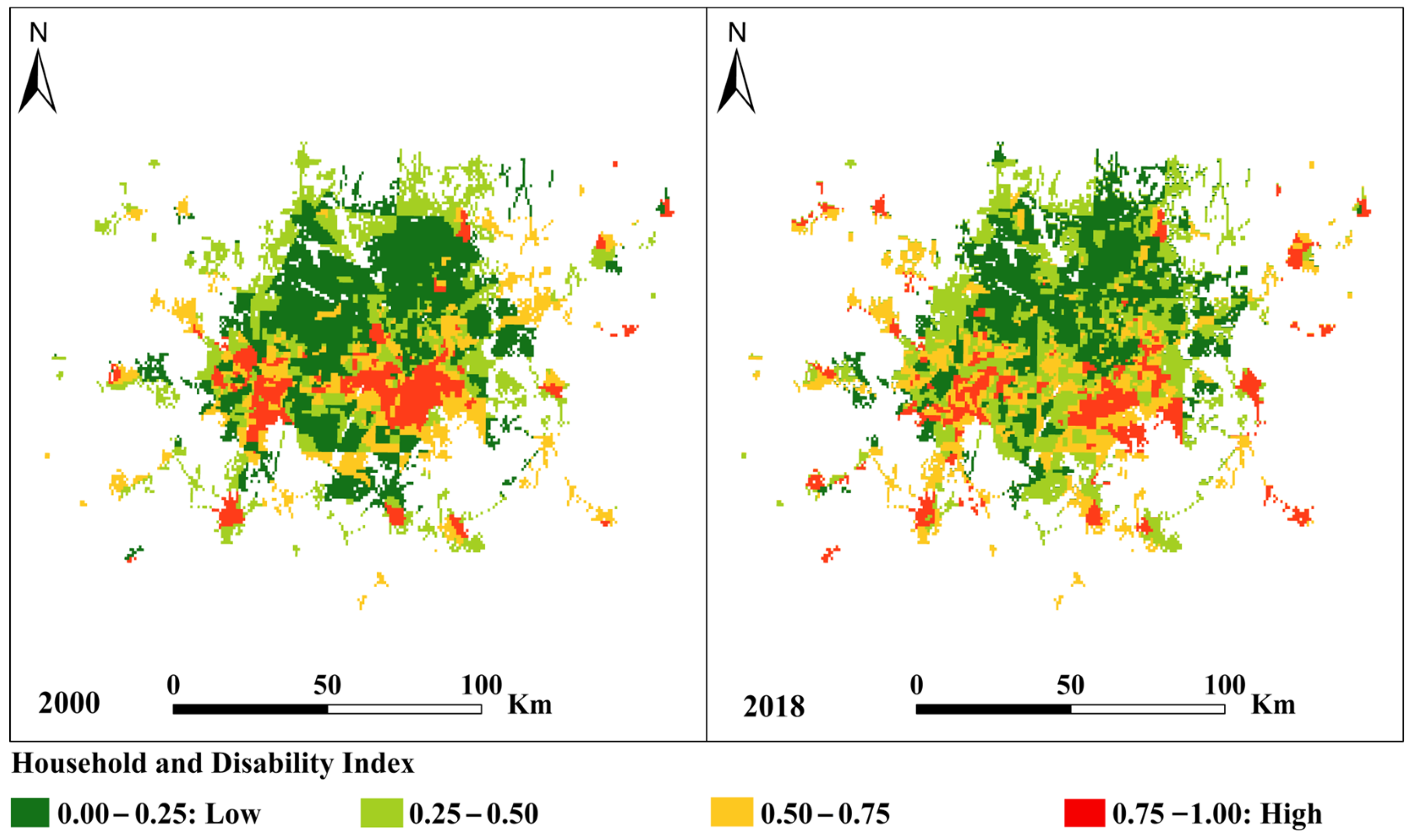
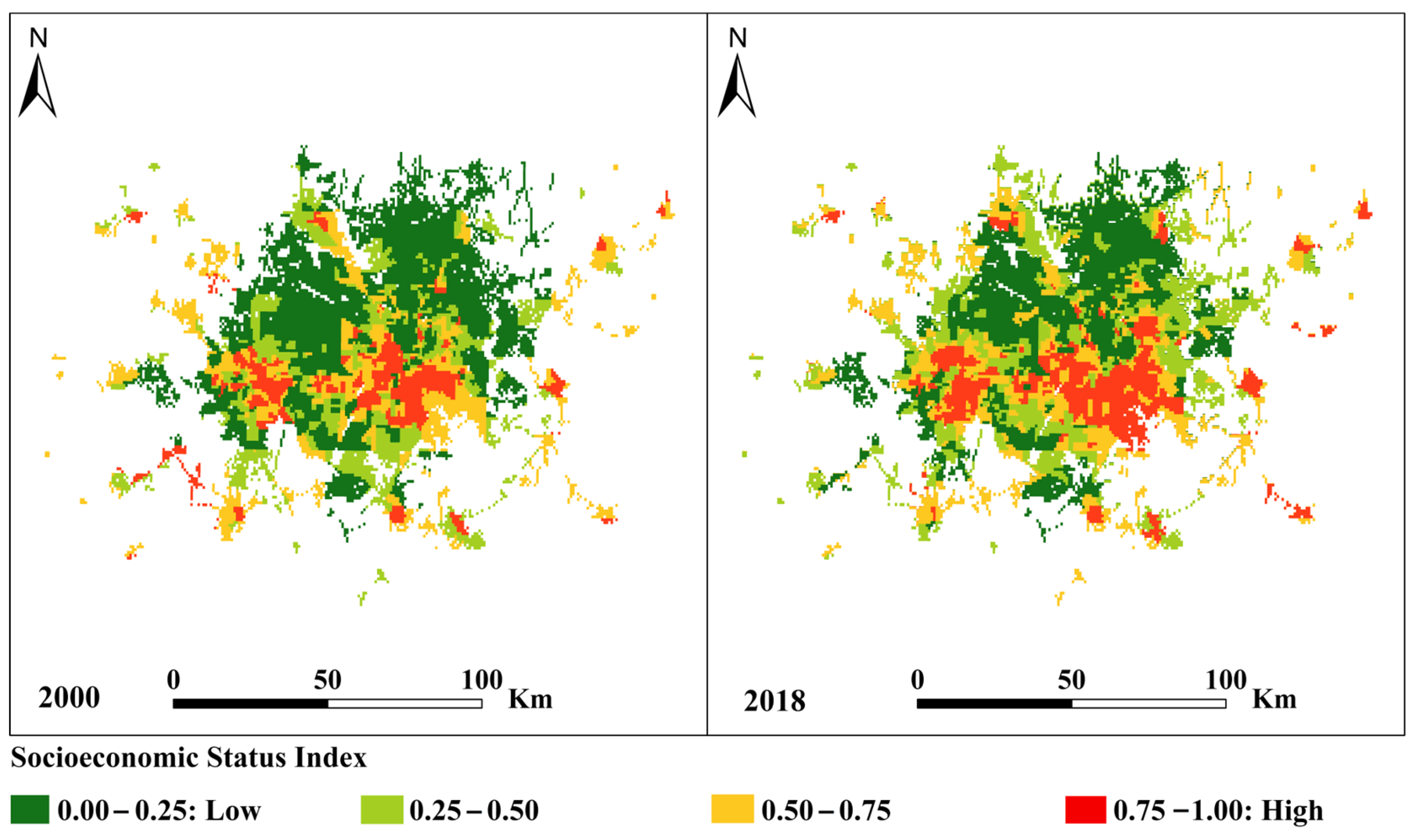
37]. Gridded SEDAC data include information about housing and transportation, household and disability, socioeconomic status, and overall social vulnerability, which is defined as the degree to which a household or community suffers or may suffer from one or more socioeconomic issues such as poverty, unemployment, educational attainment, linguistic isolation, or the percentage of income spent on housing [40,41] at the household level [37,42].
Finally, high spatial resolution gridded global climate data, WorldClim, has been developed from downscaled Climatic Research Unit (CRU) Time-Series (TS) version 4.03 [43] by the CRU, University of East Anglia, and corrected for bias with WorldClim 2.1 [44]. The Worldclim 1.4 climate dataset is based on the interpolation of point observations from meteorological stations, which regionalizes monthly observational data of precipitation and temperature using a thin plate smoothing interpolation algorithm and latitude, longitude, and elevation as statistical predictor variables [45]. Previous studies [46,47] have noted that the WorldClim remotely sensed temperature and precipitation data improve species distribution modeling and are suitable for ecological modeling studies, though the assessment of freely available WorldClim datasets, their computation methods, coherent limitations, and potential inaccuracies remain largely out of focus [48].

1.3. Objectives

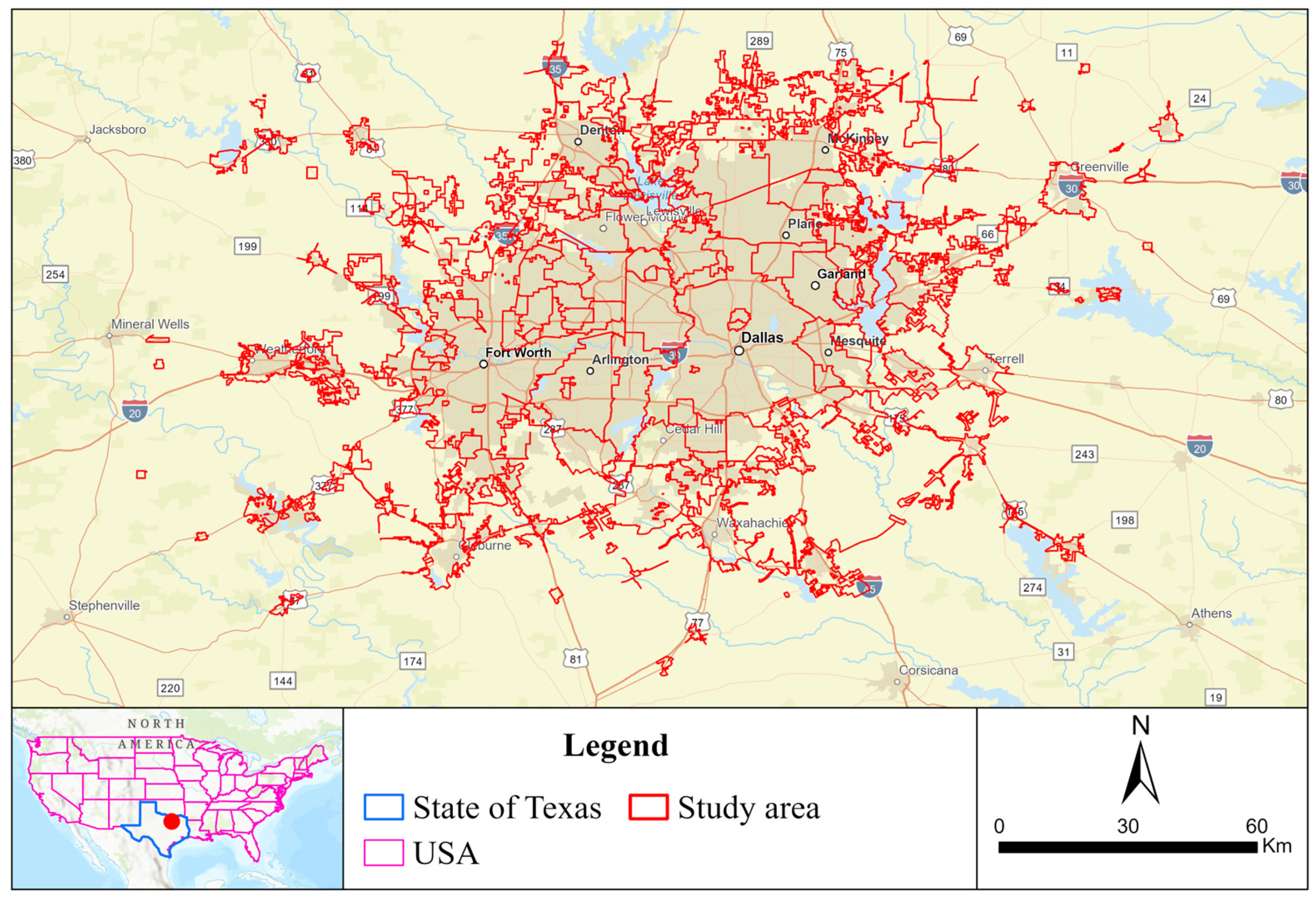
Despite the existence of these freely available remotely sensed LCLU, socioeconomic, and climate data, no studies have investigated the relationships between LCLUC and their drivers, particularly in large urban areas. This study aimed to assess the relationship of LCLUC with socioeconomic and climatic drivers based on correlation and multiple regression models to demonstrate that RS-derived datasets of LCLUC correspond to changes in socioeconomic and climatic factors in a rapidly urbanizing area.

2. Materials and Methods

2.1. Study Area

This study covers 201 cities in the Dallas-Fort Worth (DFW) metropolitan area in the state of Texas, USA (Figure 1). DFW, known for its sweeping suburban growth, is the largest (24,050.63 km2 across 12 counties), fourth-most-populated (7.8 million), and one of the fastest-growing urban regions in the U.S. Major cities in terms of population and area in the DEW include Dallas, Fort Worth, Arlington, Plano, and Irving. The DFW metropolitan area has a humid subtropical climate with hot and humid summers, although low humidity more characteristic of a desert climate can occur at any time of the year. High temperatures occur during July and August, with an average daily maximum of 35 °C and an average low of 24 °C. Winters in the DFW area are cool and mild, with occasional cold spells. January is typically the coldest month, with an average daytime high of 14 °C and a nighttime low of 2 °C, and the average annual precipitation in the DFW area is 993 mm [49,50,51].

2.2. Land Cover–Land Use Data

The NLCD of the study area was obtained from the MRLC Consortium (https://www.mrlc.gov/, accessed on 15 August 2022). The data for LCLUC analyses consisted of the NLCD for the period of 2001–2019. These data include NLCD 2001, NLCD 2006, NLCD 2011, NLCD 2016, and NLCD 2019 at 30 m spatial resolution. The NLCD 2001 and NLCD 2019 datasets were used to calculate LCLU classes and changes in the study area from 2001 to 2019, as described in Section 2.5.

2.3. Socioeconomic Data

The socioeconomic data of the study area was obtained from the SEDAC (https://doi.org/10.7927/6s2a-9r49, accessed on 15 August 2022). Socioeconomic factors included housing and transportation, household and disability, socioeconomic status, and overall social vulnerability index (SVI). The SVI, a composite measure assessing the resilience of communities when confronted with external stresses on human health, such as natural or human-caused disasters, used in this study was obtained from the CDC’s SVI, which relies on publicly available U.S. Census data to assess the social vulnerability of each census tract. The SVI ranks tracts based on 15 social factors, such as poverty, lack of vehicle access, and crowded housing, and groups them into four categories: socioeconomic status, household composition/disability, minority status/language, and housing type/transportation. The CDC provides the SVI for the entire U.S. as well as for each state, with census tracts ranked against others within the state. The SVI is calculated by summing scores for each factor and converting them into a percentile rank between 0 and 1, with higher scores indicating greater vulnerability [52].
The U.S. socioeconomic datasets (e.g., socioeconomic status) in SEDAC contain gridded layers for the overall Centers for Disease Control and Prevention (CDC) for the years 2000, 2010, 2014, 2016, and 2018. The gridded layers’ values range between 0 and 1 depending on their percentile position among all census tracts in the U.S., with 0 representing the lowest value/vulnerability census tracts and 1 representing the highest value/vulnerability census tracts. SEDAC has gridded these vector inputs to create 1 km spatial resolution raster surfaces, allowing users to obtain socioeconomic metrics for any user-defined area within the U.S. Utilizing inputs from CIESIN’s Gridded Population of the World (GPW), Version 4, Revision 11 (GPWv4.11), a mask is applied for water and, optionally, for no population. The data are provided in two different projection formats: NAD83 as a U.S.-specific standard and WGS84 as a global standard [53]. The 2000 and 2018 datasets, the closest years to the NLCD 2001 and NLCD 2019 datasets, were used to calculate socioeconomic variables and their changes in the study area from 2000 to 2018.
The population data of the study area was obtained from CIESIN’s GPW (https://doi.org/10.7927/H4JW8BX5, accessed on 10 February 2023). For developing GPW, population input data are acquired using the most spatially explicit resolution accessible from the outcomes of the 2010 round of population and housing censuses, which were conducted between 2005 and 2014. The input data are extrapolated to obtain population projections for the years 2000, 2005, 2010, 2015, and 2020. A set of projections, including historical and future population projections, was adjusted to the national level, from the United Nations World Population Prospects [46]. GPW are available in a variety of formats (ASCII, GeoTIFF, and NetCDF) and resolutions (2.5 arc-minute, 15 arc-minute, 30 arc-minute, and 1 degree). We utilized the latest version of GPW (GPWv4) in ASCII format, with a spatial resolution of 30 arc-seconds (approximately 1 km at the equator), to obtain population data for 2000 and 2020—the closest available years to the NLCD datasets of 2001 and 2019.

2.4. Climatic Data

The climatic data of the study area for the years 2000 and 2018, the closest years to the NLCD datasets of 2001 and 2019, were obtained from WorldClim (https://www.worldclim.org/data/worldclim21.html, accessed on 15 August 2022). The variables used for this study are monthly minimum temperature (°C), monthly maximum temperature (°C), and monthly total precipitation (mm). The spatial resolution is 2.5 min (~21 km2). Each download is a “zip” file containing 120 GeoTiff (.tif) files for each month of the year (January is 1; December is 12), for a 10-year period. Since the climatic data for each month of a year were separate rasters, we combined monthly gridded data from all 12 months of a year to compute the monthly averages for minimum temperature, maximum temperature, and precipitation for that year. These new variables were named monthly average minimum temperature, monthly average maximum temperature, and monthly mean precipitation. The averaged raster datasets were utilized in the change detection analysis.

2.5. Image and Spatial Analyses

To identify changes in LCLU, socioeconomic, and climatic data, image and spatial analyses were used. To achieve this, the raster layers of NLCD, socioeconomic, and climatic data were first clipped and spatially joined to the study area. The layers were then re-projected and resampled to retrieve accurate area information. Because of differences in spatial resolution among the different datasets, the data were averaged for each municipality (city) within the DFW metroplex. The categorical change detection techniques were next used to detect the type of change (positive/gain or negative/loss) that occurred between two raster layers from 2000–2020. Categorical change detection techniques identify differences between two categorical or thematic rasters, with the output highlighting every class transition that occurred. For instance, a class labeled “Forest > Developed” signifies a change from “Forest” in Raster 1 to “Developed” in Raster 2 over the specified period.
The gridded datasets composed of calculated change values between each date were converted to points using the Raster to Point tool to extract the mean digital number (DN) values of each pixel for the polygon of each city, which was obtained from the Texas Department of Transportation (https://gis-txdot.opendata.arcgis.com/datasets/09cd5b6811c54857bd3856b5549e34f0_0/explore?location=31.060571%2C-100.168292%2C7.39, accessed on 20 September 2022). The mean DN value of the raster layers for each city polygon was finally computed. Thus, the resulting attribute table for the polygon of each city included newly added DN values of the raster layers of NLCD, socioeconomic, and climatic data. These image and spatial analyses were all carried out using the extract toolset (clip analysis), image analyst tools (change detection analysis), spatial analyst tools (reclassification), and overlay toolset (spatial join analysis) in ArcGIS Pro 3.0.1 [54].

2.6. Statistical Analyses

We used 74 cities out of a total of 201 located within the metroplex boundary for statistical analysis due to DN values of socioeconomic and climatic variables having zero or null values. For these 74 remaining municipalities, we first used Pearson’s correlation coefficient analysis to examine the relationships between LCLUC from 2001–2019 and changes in each socioeconomic and climatic variable from 2000–2018 (except population, which was from 2000–2020), separately. We then used a multiple regression analysis to evaluate how LCLUC may affect socioeconomic (population, housing and transportation, household and disability, socioeconomic status, and SVI) and climatic (monthly average minimum temperature, monthly average maximum temperature, and monthly mean precipitation) variables. Prior to these statistical analyses, all variables were checked for the assumptions of normality and linearity. Since some of the variables did not meet the assumptions of normality and linearity, they were normalized using appropriate transformation techniques (e.g., logarithm). Variance Inflation Factors (VIFs) were employed to detect multicollinearity in the multiple regression model, quantifying the extent to which the variance of a regression coefficient was inflated due to linear relationships among predictors. Our analysis indicated that all VIFs were well below the commonly accepted threshold of 5, suggesting that multicollinearity did not significantly impact our model’s estimates. All statistical analyses were conducted using R 4.2.1 [55].

3. Results

3.1. Land Cover—Land Use: Status and Changes

3.1.1. Land Cover—Land Use Status for 2001 and 2019

The LCLU classes from 2001 and 2019 are shown in Table 1. In 2001, the extent of human-dominated, non-vegetated, and vegetated areas was similar in the DFW metroplex, with areas of 3896.29 and 3898.01 km2, respectively. However, in 2019, the extent of human LULC increased to 4306.55 km2, which coincided with a decrease in vegetation cover to 3387.08 km2. Mapped NLCD LULC data show that the human-dominated classes expanded from the core of the DFW outward, mostly replacing herbaceous and shrub/scrub vegetation toward the edge of the study area (Figure 2). The natural non-vegetation areas (e.g., Barren Land, Open Water), changed from 339.56 to 372.32 km2 from 2001 to 2019, primarily associated with increased open water in the study area. Changes in open water are likely associated with differences in reservoir storage that were lower in 2001 than in 2019.

3.1.2. Land Cover—Land Use Change from 2001 to 2019

The NLCD LCLUC gains and losses are shown in Table 2, calculated for the period of 2001–2019. These results showed that 15.56% (1265.76 km2) of the study area has seen changes (gains and losses), while 84.44% (6868.08 km2) of the study area has experienced “no change in LCLU”. Areas classified as human non-vegetation expanded their area with a net change of 848.15 km2. Within the human classes, the Developed—Medium intensity increased the most from 2001 to 2019 (487.47 km2). This was followed by Developed—High and Developed—Low Intensity, with increased areas of 238.20 and 116.70 km2, respectively. These human land cover conversions were offset by a loss in vegetation cover (999.75 km2). Of the vegetated classes, most of the decrease was for the Herbaceous class (636.82 km2 loss), followed by Deciduous Forest (108.19 km2 loss), and Cultivated Crops, with a loss of 59.79 km2.
In Figure 3, mapped pixels showing the spatial distribution of NLCD LCLUC gains, or pixels that changed from one class to another, are illustrated. This supports the overall increase in human-dominated LULC and illustrates an expansion of these land uses towards the outer areas of the study area. Likewise, the mapped overall losses are shown in Figure 4. These confirm that much of the gain in human-dominated classes was associated with the loss of vegetation. Lastly, much of the center of the DFW metroplex has experienced no change, remaining urbanized in LCLU from 2001–2019.

3.2. Socioeconomic and Climatic Variables: Status and Changes

3.2.1. Population

In Figure 5, the mapped population count (number of persons per km2) is shown for the study area for 2000 and 2020. In 2000, the most populated areas (>1000 persons per km2) accounted for 95.45% of the DFW metroplex. This includes the largest cities comprising the metroplex (e.g., Dallas, Fort Worth, Arlington), while 4.55% of the study area had low to moderate intensity (1 to 250 people persons per km2), which includes smaller municipalities (e.g., Prosper, Neylandville, Corral).
When assessing the change in population between 2000 and 2020, we found that 79.70% of the area remained relatively unchanged between the two years of analysis (Table 3). For example, those parts of the metroplex that had a moderate population count (25 to 250 persons per km2) remained almost the same from 2000 to 2020. Moreover, 20.30% of population changes that occurred were associated with the conversion of low-populated areas (<1 to 5 persons per km2) to moderately populated areas (>1000 persons per km2). However, significant spatial shifts in population density were observed, particularly in suburban and peri-urban areas. Specifically, 20.30% of the population changes were associated with the conversion of low-populated areas (<1 to 5 persons per km2) to moderately populated areas (>1000 persons per km2). This suggests that suburban expansion and increased housing development have played a key role in reshaping population distribution over time. The observed increase in population density in previously low-population regions may be driven by factors such as urban sprawl, infrastructure development, and economic growth, leading to the transformation of rural or undeveloped lands into residential and commercial zones.

3.2.2. Housing and Transportation

The mapped distribution of housing and transportation density is shown in Figure 6 and Table 4. for the DFW metroplex from 2000 to 2018. In 2000, 38.05% of the study area had a low index (<0.25) in terms of housing and transportation, while 17.47% of the study area had a high index (>0.75). However, most of the study area (44.48%) had an intermediate housing and transportation index (0.50–0.75). In other words, most of the research areas had a moderate index of housing and transportation structures. In 2018, the apportionment was relatively similar, though with a decrease in the low index of housing and transportation (35.59%), accompanied by a slight increase in the moderate index of housing and transportation (47.07%). The area of high-index structure for 2018 was like that of 2000, accounting for 17.37% of the study area. These results indicate that there was a visible shift in the spatial distribution of housing and transportation density, particularly in the northwestern part of the study area, where a decline from high to low index values was observed. This change may be attributed to factors such as suburban expansion, economic shifts, or zoning policies that influenced land-use patterns. It is possible that some high-density residential or transportation zones transitioned to lower-density areas due to redevelopment, shifts in infrastructure investment, or changes in housing demand. Additionally, this region might have experienced a decline in transit accessibility or an increase in vacant or underutilized land, leading to a decrease in the housing and transportation index.

3.2.3. Household and Disability

In Figure 7, the household and disability indexes derived from NASA SEDAC data are shown for 2000 and 2018. In 2000, 40.83% of the study area had low levels (<0.25) of household and disability, 11.88% of the study area had high index values (0.75 to 1.0), and the remaining portion of the metroplex (47.28%) had moderate values. In 2018, fewer areas had either low (32.74%) or high (13.31%) household and disability index values, associated with a greater area with moderate values (53.96%). Regarding changes in the household and disability status over time, approximately 45.44% (3695.80 km2) of the study area maintained a consistent status with “no change” from 2000 to 2018 (Table 5). Among the different intensity classes, class 2, characterized by a 0.25–0.50 intensity in household and disability, observed the most significant positive change with a gain of 355.94 km2. This suggests an overall shift toward moderate index values, possibly due to improved access to social services, demographic shifts, or changes in housing patterns that influenced household composition and disability prevalence. On the other hand, class 1, representing a 0–0.25 intensity in household and disability, experienced the highest negative change, with a loss of 630.84 km2 (Table 5). This decline in low-intensity areas may indicate that regions previously characterized by lower household and disability index values have undergone socioeconomic transformations, potentially due to urban development, increased housing density, or changes in population health dynamics. The shift away from the lowest index category further highlights a redistribution of household and disability characteristics across the metroplex.

3.2.4. Socioeconomic

Mapped index values of socioeconomic status in the study area for 2000 and 2018 are shown in Figure 8. These data illustrate that the study area was dominated by low socioeconomic index values in 2000, accounting for 46.52% of the DFW metroplex. Of the remaining area, 10.98% had high values (0.75–1.0), with the remaining portions (42.50%) mapped with moderate socioeconomic status. In 2018, the distribution of socioeconomic status values significantly changed across the entire study area, with areas of low values decreasing to 34.99% of the area; 48.65% had moderate values, and 16.36% of the area had high values. These changes represented an 11.53% decrease in low socioeconomic index values from 2000–2018 in contrast to a 5.38% and 6.15% increase for moderate and high values, respectively (Table 6). This shift in socioeconomic status suggests a gradual improvement in overall economic conditions, likely driven by urban development, infrastructure investments, and demographic changes. The decline in low socioeconomic index values may indicate economic growth, job creation, and gentrification in certain areas, pushing previously low-status regions into the moderate or high index categories.

3.2.5. Overall Social Vulnerability

The indices for social vulnerability across study areas for 2000 and 2018 are mapped and shown in Figure 9. In 2000, 39.43% of the study area had low overall SVI values, with 13.25% of the study area having high values. The remaining 47.33% of the metroplex had a moderate overall social vulnerability status. In 2018, the distribution of overall social vulnerability indices somewhat changed across the entire study area, with low overall SVI values observed in 33.92% of the study area (5.51% decrease), 45.67% with moderate values (1.66% increase), and 20.41% of the area with the highest social vulnerability value (7.16% increase). Regarding overall social vulnerability, over 55.07% (4478.99 km2) of the study area had “no change” in terms of overall social vulnerability (Table 7). This stability in a significant portion of the study area suggests that while changes have occurred, large sections of the metroplex have retained their social vulnerability status, potentially due to persistent structural inequalities or stable economic conditions in those areas.

3.2.6. Monthly Mean Precipitation

Mapped monthly means precipitation (mm/month) for the study area from 2001 and 2018 is shown in Figure 10. These data show that precipitation generally increases from west to east across the DFW metroplex. In 2001, precipitation ranged from 67.21 to 112.34 mm. Most of the study areas (49.76%) exhibited a mean precipitation value of 80 mm. In contrast, only 1.29% of the area, situated in the northeastern section, recorded a monthly mean precipitation exceeding 100 mm. For 2018, increased precipitation was found across the metroplex, with areas with high monthly mean precipitation increasing from 1.29% to 6.80%. The areas with moderate monthly mean precipitation, particularly those with 80–90 mm of monthly mean precipitation, increased significantly from 10.14% in 2001 to 27.36% in 2018 (Table 8).

3.2.7. Monthly Average Maximum Temperature

Mapped monthly average maximum temperatures (°C) for 2001 and 2018 are shown in Figure 11. These show that in 2001, the average maximum temperature ranged from 23.20 to 25.20 °C, with 76.01% of the study area having values of 24.5 °C. Only 0.48% of the study area experienced monthly average maximum temperatures of >25 °C. In 2018, more areas had higher monthly average maximum temperatures. The proportion of the metroplex with monthly average maximum temperatures over 25 °C increased from 0.48% to 68.92% (Table 9) in 2018, while average maximum temperatures of 24.5 °C decreased from 76.01% to 5.96%. This pattern suggests a shift toward generally higher maximum temperatures across the study area, likely influenced by urbanization, land surface changes, and increased heat absorption from impervious surfaces. The spatial distribution of these changes appears to resemble a heat island effect, particularly in urbanized areas with high population density and extensive infrastructure development. The concentration of high maximum temperatures in specific zones may also be attributed to localized land cover transformations, such as reduced vegetation and increased built-up areas, which enhance heat retention.

3.2.8. Monthly Average Minimum Temperature

The monthly average minimum temperature (°C) for 2001 and 2018 is mapped and shown in Figure 12. The data show that minimum temperatures ranged from 11.40 °C to 13.77 °C. In 2001, 22.38% of the study area had monthly average minimum temperatures below 12 °C, 20.93% of the study area had temperatures above 13 °C, and 56.68% of the area ranged between 12 and 13 °C. In 2018, areas with monthly average minimum temperatures of >13 °C increased from 20.93% in 2001 to 35.10%, while areas below 12 °C decreased from 22.38% in 2001 to 14.49% in 2018 (Table 3). Areas with moderate monthly average minimum temperatures, between 12 and 13 °C, showed a minor shift, with a 6.28% decrease from 56.68% in 2001 to 50.40% in 2018 (Table 10). Unlike the maximum temperature distribution, the minimum temperature changes exhibit a distinct southwest-to-northeast gradient. This pattern may be influenced by prevailing wind directions, elevation differences, or proximity to water bodies, which can create localized cooling effects. Additionally, rural-to-urban thermal contrasts may contribute to the observed distribution, as areas with more vegetation cover and open spaces tend to experience lower minimum temperatures compared to densely developed urban zones. The differences in the spatial patterns of minimum and maximum temperature changes highlight the role of both large-scale climatic influences and localized urban effects in shaping temperature dynamics across the region.

3.3. Relationships Between LCLUC with Socioeconomic and Climatic Variables

Table 11 presents the results of the correlation analysis for LCLUC and changes in socioeconomic variables. Results showed that LCLUC had weak but significant relationships with changes in all socioeconomic and climatic variables, except for the overall social vulnerability change and the monthly average maximum temperature change (Table 11). Results further confirmed that LCLUC was negatively related to population change, monthly average minimum temperature change, and monthly mean precipitation (Table 11), whereas it was positively related to housing and transportation change, household and disability change, and socioeconomic status change (Table 11). There was no significant relationship between LCLUC, overall social vulnerability change, and monthly average maximum temperature change.

3.4. Multiple Linear Regression Modeling of Land-Cover and Land-Use Change

The relationship between LCLUC and its socioeconomic and climatic drivers, using a multivariate regression model approach, showed a significant but weakly predictive association (R2 = 0.36). Results showed that LCLUC was best explained by population change, housing and transportation change, household and disability change, socioeconomic status change, monthly minimum temperature change, and monthly mean precipitation change (Table 12). Of these variables, changes in housing and transportation were the most significant based on the p-value calculated from the regression model.

4. Discussion

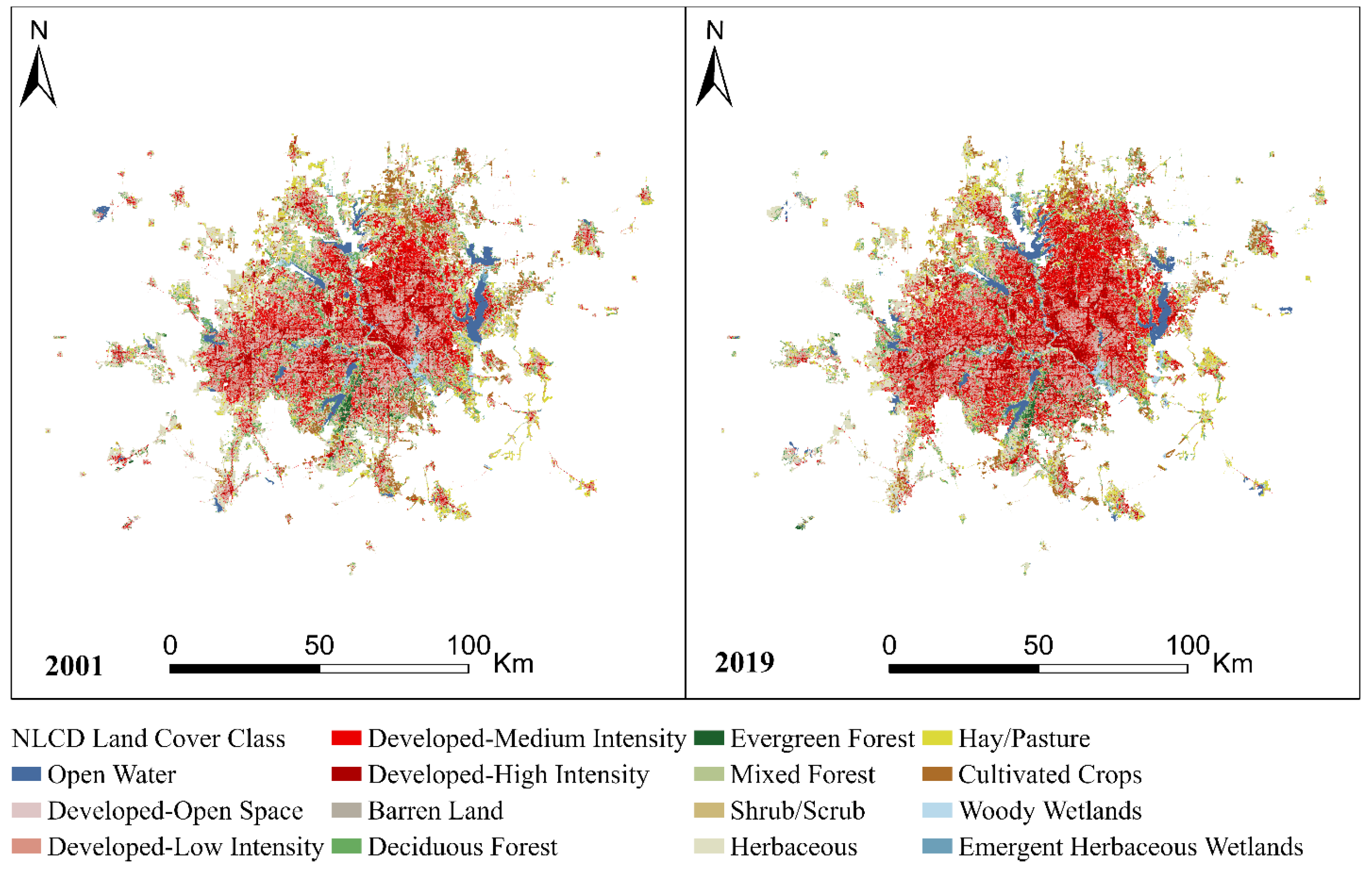
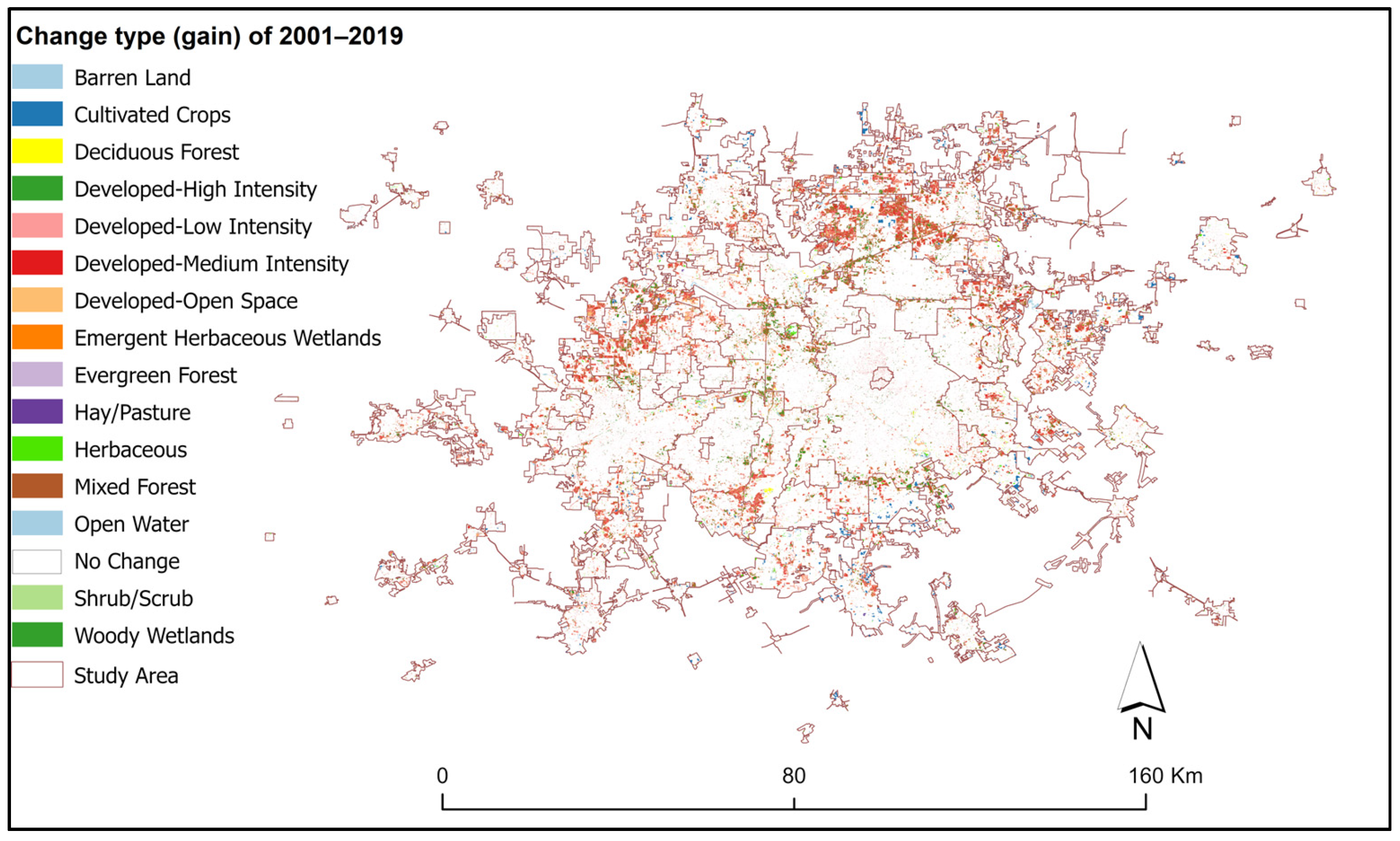
This study sought to identify LCLUC and changes in the context of socioeconomic and climatic drivers by utilizing a publicly available time series of RS datasets in one of the largest and most populated metropolitan areas (DFW) in the U.S. We found that growing socioeconomic pressures in this urbanized area coupled with on-going climate change have affected LCLUC, much to the diminishment of vegetated area, resulting in rapid global environmental change [13]. Addressing these threats will support sustainable land management, which will significantly enhance the achievement of sustainable development goals. The spatial analysis of LCLUC highlights key patterns across the study area. Specifically, our results indicate that LCLUCs are not evenly distributed but rather exhibit distinct spatial patterns driven by underlying socioeconomic and climatic factors. For example, areas experiencing high urbanization and economic activity show greater LCLUCs, while regions with lower development pressures exhibit relatively stable land cover trends. The spatial patterns of temperature changes also suggest the presence of urban heat island effects, particularly in highly developed areas. These spatial insights provide a deeper understanding of the complex interactions between LCLUC, socioeconomic factors, and climate.
Our findings that LCLUC, socioeconomic, and climatic variables are correlated in line with recent studies examining these correlations on various regional to global scales [2,3,12,56,57,58]. This is consistent with the findings of Ref. [58], which found that 60% of all LCLUC is caused by direct human-related factors and 40% by indirect causes such as climate change. Similarly, Ref. [2] confirmed that socioeconomic factors are closely associated with changes in LCLU status. As a result, areas experiencing high intensity in terms of socioeconomic factors, such as high demands for housing and transportation or a higher rate of household or socioeconomic status, are at a high risk of LCLUC. Our spatial analysis further reveals that the most significant LCLUC transformations have occurred in the peripheral urban areas, particularly in zones with rapid residential and commercial expansion. This suggests that spatially targeted policies may be necessary to manage land development sustainably. However, the low regression coefficients observed in our study may be justifiable given the relatively short analysis period, the variability in LCLU during this time, and the limited sample size. In addition, other socioeconomic (e.g., GDP) and climatic (e.g., annual temperature) factors may also be important or more directly associated with LCLUC, for which we lacked gridded observations to include in our study. Given the importance of gridded observations in analyzing LCLUC, future studies should integrate historical gridded LCLU datasets, which are now widely available through various international sources. Incorporating these datasets will enhance the precision of LCLUC assessments and strengthen predictive modeling in this field.
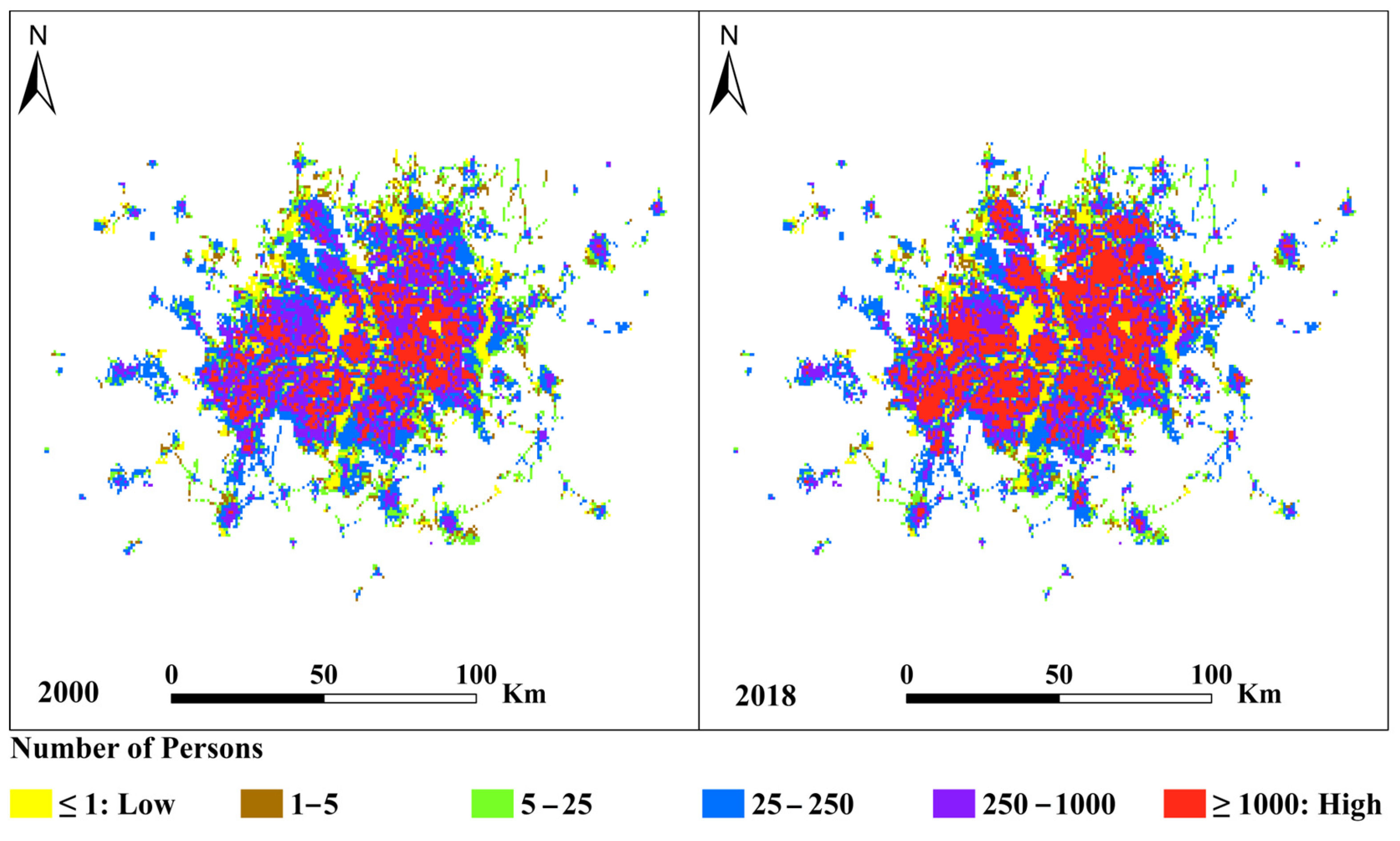
Our study found that, of all studied socioeconomic factors, population change had a negative relationship with LCLUC. This opposes the common perception that population change and LCLUC should be positively correlated, as well as the findings of previous studies [2,59]. Although overall population numbers are often positively related to LCLUC, some research indicates that this overall relationship depends on a variety of factors (e.g., land settlement policies, and market forces). In other words, the effects of population change on LCLUC must be understood in the context of other drivers of LCLUC, indicating that population changes can affect LCLUC differently in different regions [60]. This negative relationship between LCLUC and population changes in our study may be due to the heterogeneous effects of human activities on LCLUC, as previously demonstrated by Ref. [12]. A heterogeneous and opposing direction of change pattern between LCLU and population was observed in the study area, indicating that a high changing rate of population occurred in areas close to the center of DFW and places far away from the central areas. However, more areas had LCLUCs far away from the central parts of DFW. Previous studies have revealed that most human activities take place close to metropolitan centers because of the convenience of access to markets and agricultural inputs [61,62]. Our spatial analysis suggests that this negative relationship may be influenced by differential land use dynamics within the study area. For example, areas with high population growth near the DFW metropolitan center may not exhibit large-scale LCLUC because of pre-existing urban infrastructure, whereas more extensive LCLUCs are observed in suburban and exurban areas undergoing rapid development. This highlights the importance of spatially contextualizing the relationship between population change and LCLUC.
We also found no correlation between LCLUC and SVI change. While previous studies [63,64] have indicated that socioeconomic vulnerability change and land cover indicators could be related to one another in natural ecosystems (e.g., rangelands), it seems that no such relationship exists between them in our study area. Our study’s results differ from their findings, possibly because the scale, complexity of the socioeconomic setting, and land use type of an area, whether it is a natural ecosystem or built-up land, can determine the relationship between LCLUC and its driving forces [16]. In addition, the SEDAC’s social vulnerability is calculated using only a few variables, possibly missing important socioeconomic elements. According to Ref. [63], social vulnerability alone has little to no direct connection with LCLUC. Social and economic vulnerability, when examined as socioeconomic vulnerability, can have a stronger correlation with LCLUC than either social or economic vulnerability alone. Socioeconomic vulnerability can act as a catalyst for LCLUC rather than its primary cause. According to Refs. [65,66], LCLUC tends to increase along with the increase in socioeconomic vulnerability if there is a high level of socioeconomic activity in an area. High socioeconomic activity levels are indicators of how dependent a community is on natural resources [16,67]. However, our spatial analysis further showed that areas with higher social vulnerability did not necessarily exhibit corresponding LCLUC trends. This suggests that other localized factors, such as zoning policies or economic diversification, may mitigate the expected impact of social vulnerability on land use change. This could explain why this study’s results differ from those of previous studies. Currently, the only major natural resources affecting direct economic activity in DFW are water and petroleum extraction from hydraulic fracturing [68], both of which are unlikely to affect appreciable areas of land cover and use.
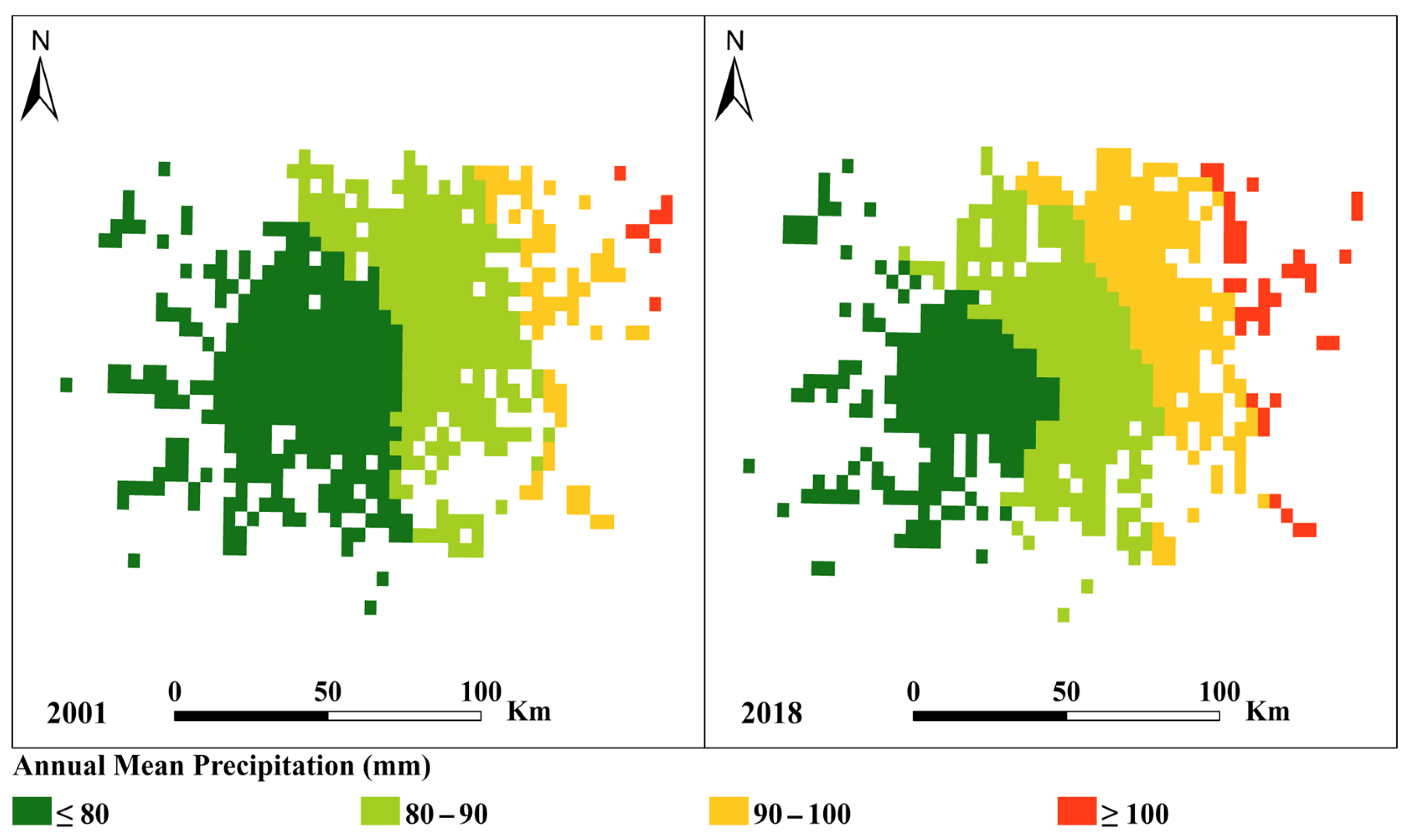
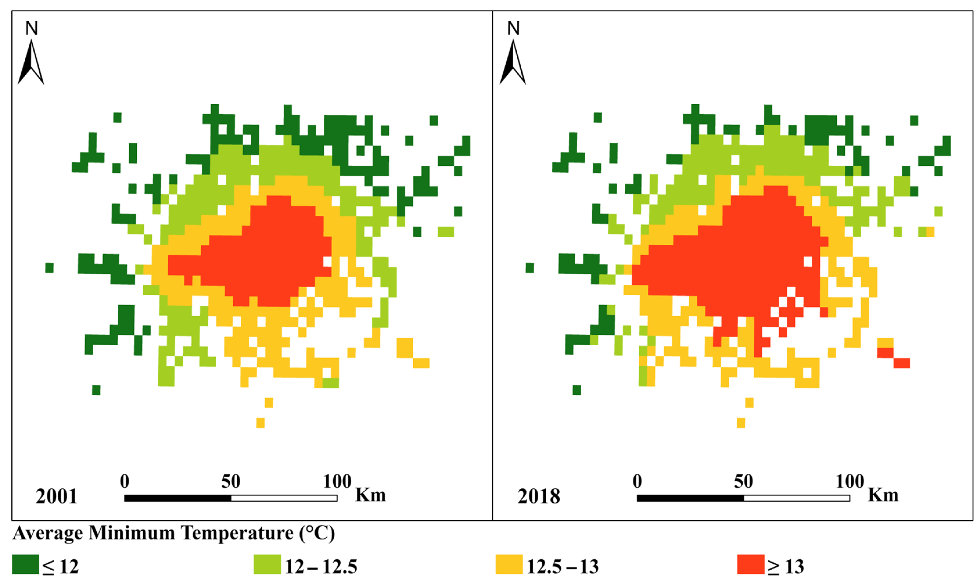
Of the climate variables, such as monthly average minimum temperature and mean precipitation change, these were found to be negatively correlated with LCLUC. This is consistent with previous research [2,16,61]. This could be because most land use systems need certain temperature and precipitation conditions. High temperatures and low precipitation, for example, might well relate to drier conditions that are inappropriate for some land use types, including inhabited areas [68,69]. However, this study only considered the monthly precipitation and temperature values for two discrete years, 2001 and 2018. However, based on historical temperature values from DFW dating to 1899, average annual temperatures have been increasing by 0.1 °C per decade (https://www.weather.gov/fwd/dmotemp) (accessed on 15 August 2023).
Finally, this study demonstrated that the remote sensing datasets from NASA, the MRLC Consortium, and WorldClim with high spatial resolution, which were used in this study, are essential for studying trends and causes of LCLUC. However, LCLUC drivers have been widely perceived using data obtained through social surveys or field studies [70,71]. Social surveys and field studies are simple to conduct but time- and money-consuming, and they are unlikely to be derived directly from remote sensing. Future studies should continue to use such datasets in assessing LCLUC, incorporating more detailed socioeconomic data, such as those from federal census information, and an expanded set and temporal sampling of climatic information. Additionally, future research should further integrate spatial analysis techniques to better understand the geographic variations of LCLUC and its drivers at finer scales.

5. Conclusions

To the best of our knowledge, this is the first study to assess the relationship between LCLUC and its socioeconomic and climatic drivers using a time series of RS-gridded datasets of agencies such as NASA in an important metropolitan area such as DFW. We concluded that, firstly, LCLUC is driven by a combination of both socioeconomic and climatic drivers. Secondly, LCLUC was negatively affected by changes in population, monthly average minimum temperature, and precipitation, whereas it was positively affected by changes in housing and transportation, household and disability status, and socioeconomic status. Finally, we concluded that the remote sensing-gridded products from NASA, the MRLC Consortium, and WorldClim could offer significant and spatially specific information in addressing socioeconomic and climatic factors affecting LCLUC. These freely available datasets may be used to save time and money when dealing with the LCLUC phenomenon around the world. The methodology used in this study is transferable to other regions, particularly other regions of the conterminous United States because gridded datasets for most of the socioeconomic and climatic factors with a spatial and temporal resolution are available from the agencies mentioned in this study (e.g., NASA’s SEDAC, WorldClim) that can be used in conjunction with national or global LCLUC datasets to study potential relationships between them. Additionally, several international studies, including those conducted by Chinese scholars, have applied various spatial and statistical models (e.g., random forest, regression tree, logistic regression model) to analyze LCLUC patterns. Incorporating findings from these studies can help improve the robustness of LCLUC assessments and provide broader insights into how different modeling approaches perform across various geographic regions. Future research should integrate such methodologies to strengthen comparative analyses and enhance predictive modeling of LCLUC at regional, national, and global scales before generalizing this study’s findings.

Author Contributions

Conceptualization, A.R. and J.D.W.; methodology, A.R. and J.D.W.; software, A.R.; validation, A.R. and J.D.W.; formal analysis, A.R.; investigation, A.R.; resources, A.R.; data curation, A.R.; writing—original draft preparation, A.R.; writing—review and editing, J.D.W.; visualization, A.R.; supervision, A.R.; project administration, A.R. All authors have read and agreed to the published version of the manuscript.

Funding

This research received no external funding.

Data Availability Statement

All the data used in this study are publicly available and can be downloaded from the following links: (1) LCLUC data: https://www.mrlc.gov/, accessed on 15 August 2022. (2) Socioeconomic data: https://doi.org/10.7927/6s2a-9r49, accessed on 15 August 2022. (3) Population data: https://sedac.ciesin.columbia.edu/data/collection/gpw-v4, accessed on 10 February 2023. (4) Climatic data: https://www.worldclim.org/data/worldclim21.html, accessed on 15 August 2022.

Conflicts of Interest

The authors declare no conflicts of interest.

References

  1. Foley, J.A.; DeFries, R.; Asner, G.P.; Barford, C.; Bonan, G.; Carpenter, S.R.; Chapin, F.S.; Coe, M.T.; Daily, G.C.; Gibbs, H.K.; et al. Global consequences of land use. Science 2005, 309, 570–574. [Google Scholar] [CrossRef] [PubMed]
  2. Hellwig, N.; Walz, A.; Markovic, D. Climatic and socioeconomic effects on land cover changes across Europe: Does protected area designation matter? PLoS ONE 2019, 14, e0219374. [Google Scholar] [CrossRef] [PubMed]
  3. Wang, S.W.; Munkhnasan, L.; Lee, W.K. Land use and land cover change detection and prediction in Bhutan’s high-altitude city of Thimphu, using cellular automata and Markov chain. Environ. Chall. 2021, 2, 100017. [Google Scholar] [CrossRef]
  4. Hussain, S.; Mubeen, M.; Karuppannan, S. Land use and land cover change analysis using TM, ETM+ and OLI Landsat images in district of Okara, Punjab, Pakistan. Phys. Chem. Earth Parts a/b/c 2022, 126, 103117. [Google Scholar] [CrossRef]
  5. Winkler, K.; Fuchs, R.; Rounsevell, M.; Herold, M. Spatiotemporal patterns of global land use change: Understanding processes and drivers. In EGU General Assembly Conference Abstracts; EGU: Munich, Germany, 2021; p. EGU21-14471. [Google Scholar]
  6. Opacka, B.; Müller, J.F.; Stavrakou, T.; Bauwens, M.; Sindelarova, K.; Markova, J.; Guenther, A.B. Global and regional impacts of land cover changes on isoprene emissions derived from spaceborne data and the MEGAN model. Atmos. Chem. Phys. 2021, 21, 8413–8436. [Google Scholar] [CrossRef]
  7. Bicking, S.; Burkhard, B.; Kruse, M.; Müller, F. Bayesian Belief Network-based assessment of nutrient regulating ecosystem services in Northern Germany. PLoS ONE 2019, 14, e0216053. [Google Scholar] [CrossRef]
  8. Adhikari, A.; Hansen, A.J. Land use change and habitat fragmentation of wildland ecosystems of the North Central United States. Landsc. Urban Plan. 2018, 177, 196–216. [Google Scholar] [CrossRef]
  9. Shiferaw, H.; Alamirew, T.; Kassawmar, T.; Zeleke, G. Evaluating ecosystems services values due to land use transformation in the Gojeb watershed, Southwest Ethiopia. Environ. Syst. Res. 2021, 10, 22. [Google Scholar] [CrossRef]
  10. Rimba, A.B.; Mohan, G.; Chapagain, S.K.; Arumansawang, A.; Payus, C.; Fukushi, K.; Avtar, R. Impact of population growth and land use and land cover (LULC) changes on water quality in tourism-dependent economies using a geographically weighted regression approach. Environ. Sci. Pollut. Res. 2021, 28, 25920–25938. [Google Scholar] [CrossRef]
  11. Kouassi, J.L.; Gyau, A.; Diby, L.; Bene, Y.; Kouamé, C. Assessing land use and land cover change and farmers’ perceptions of deforestation and land degradation in South-West Côte d’Ivoire, West Africa. Land 2021, 10, 429. [Google Scholar] [CrossRef]
  12. Li, Y.; Sun, Y.; Li, J. Heterogeneous effects of climate change and human activities on annual landscape change in coastal cities of mainland China. Ecol. Indic. 2021, 125, 107561. [Google Scholar] [CrossRef]
  13. Meyer, W.B.; Turner, B.L. Human population growth and global land-use/cover change. Annu. Rev. Ecol. Syst. 1992, 23, 39–61. [Google Scholar] [CrossRef]
  14. Bilsborrow, R.E.; Okoth-Ogendo, H.W.O. Population-driven changes in land use in developing countries. Ambio 1992, 21, 37–45. [Google Scholar]
  15. Jolly, C.L. Population change, land use and the environment. Reprod. Health Matters 1993, 1, 13–25. [Google Scholar] [CrossRef]
  16. Kavhu, B.; Mashimbye, Z.E.; Luvuno, L. Characterising social-ecological drivers of landuse/cover change in a complex transboundary basin using singular or ensemble machine learning. Remote Sens. Appl. Soc. Environ. 2022, 27, 100773. [Google Scholar] [CrossRef]
  17. Tian, L.; Chen, J.; Yu, S.X. Coupled dynamics of urban landscape pattern and socioeconomic drivers in Shenzhen, China. Landsc. Ecol. 2014, 29, 715–727. [Google Scholar] [CrossRef]
  18. Su, S.; Wang, Y.; Luo, F.; Mai, G.; Pu, J. Peri-urban vegetated landscape pattern changes in relation to socioeconomic development. Ecol. Indic. 2014, 46, 477–486. [Google Scholar] [CrossRef]
  19. Parcerisas, L.; Marull, J.; Pino, J.; Tello, E.; Coll, F.; Basnou, C. Land use changes, landscape ecology and their socioeconomic driving forces in the Spanish Mediterranean coast (El Maresme County, 1850–2005). Environ. Sci. Policy 2012, 23, 120–132. [Google Scholar] [CrossRef]
  20. Marsh, G.P. Man and Nature: Or Physical Geography as Modified by Human Action; Sampson Low, Son and Marston: New York, NY, USA, 1864. [Google Scholar]
  21. Sauer, C.O. Grassland, Climax, Fire, and Man. J. Range Manag. 1950, 3, 16–21. [Google Scholar] [CrossRef]
  22. Kefalas, G.; Kalogirou, S.; Poirazidis, K.; Lorilla, R.S. Landscape transition in Mediterranean islands: The case of Ionian islands, Greece 1985–2015. Landsc. Urban Plan. 2019, 191, 103641. [Google Scholar] [CrossRef]
  23. Hansen, A.J.; Piekielek, N.; Davis, C.; Haas, J.; Theobald, D.M.; Gross, J.E.; Running, S.W. Exposure of US National Parks to land use and climate change 1900–2100. Ecol. Appl. 2014, 24, 484–502. [Google Scholar] [CrossRef]
  24. Ellis, E.C.; Kaplan, J.O.; Fuller, D.Q.; Vavrus, S.; Klein Goldewijk, K.; Verburg, P.H. Used planet: A global history. Proc. Natl. Acad. Sci. USA 2013, 110, 7978–7985. [Google Scholar] [CrossRef]
  25. Tasser, E.; Leitinger, G.; Tappeiner, U. Climate change versus land-use change—What affects the mountain landscapes more? Land. Use Policy 2017, 60, 60–72. [Google Scholar] [CrossRef]
  26. Huntington, E.; Visher, S.S. Climatic Changes: Their Nature and Causes; Yale University Press: New Haven, CT, USA, 1922. [Google Scholar]
  27. Feranec, J.; Jaffrain, G.; Soukup, T.; Hazeu, G. Determining changes and flows in European landscapes 1990–2000 using CORINE land cover data. Appl. Geogr. 2010, 30, 19–35. [Google Scholar] [CrossRef]
  28. Chughtai, A.H.; Abbasi, H.; Karas, I.R. A review on change detection method and accuracy assessment for land use land cover. Remote Sens. Appl. Soc. Environ. 2021, 22, 100482. [Google Scholar] [CrossRef]
  29. Fan, M.; Chen, L. Spatial characteristics of land uses and ecological compensations based on payment for ecosystem services model from 2000 to 2015 in Sichuan Province, China. Ecol. Inform. 2019, 50, 162–183. [Google Scholar] [CrossRef]
  30. Haque, M.I.; Basak, R. Land cover change detection using GIS and remote sensing techniques: A spatio-temporal study on Tanguar Haor, Sunamganj, Bangladesh. Egypt. J. Remote Sens. Space Sci. 2017, 20, 251–263. [Google Scholar] [CrossRef]
  31. Zhan, X.; Defries, R.; Townshend, J.R.G.; Dimiceli, C.; Hansen, M.; Huang, C.; Sohlberg, R. The 250 m global land cover change product from the Moderate Resolution Imaging Spectroradiometer of NASA’s Earth Observing System. Int. J. Remote Sens. 2000, 21, 1433–1460. [Google Scholar] [CrossRef]
  32. Homer, C.; Dewitz, J.; Jin, S.; Xian, G.; Costello, C.; Danielson, P.; Riitters, K. Conterminous United States land cover change patterns 2001–2016 from the 2016 national land cover database. ISPRS J. Photogramm. Remote Sens. 2020, 162, 184–199. [Google Scholar] [CrossRef] [PubMed]
  33. Wickham, J.; Homer, C.; Vogelmann, J.; McKerrow, A.; Mueller, R.; Herold, N.; Coulston, J. The multi-resolution land characteristics (MRLC) consortium—20 years of development and integration of USA national land cover data. Remote Sens. 2014, 6, 7424–7441. [Google Scholar] [CrossRef]
  34. Wickham, J.; Stehman, S.V.; Neale, A.C.; Mehaffey, M. Accuracy assessment of NLCD 2011 percent impervious cover for selected USA metropolitan areas. Int. J. Appl. Earth Obs. Geoinf. 2020, 84, 101955. [Google Scholar] [CrossRef] [PubMed]
  35. Wickham, J.; Stehman, S.V.; Sorenson, D.G.; Gass, L.; Dewitz, J.A. Thematic accuracy assessment of the NLCD 2016 land cover for the conterminous United States. Remote Sens. Environ. 2021, 257, 112357. [Google Scholar] [CrossRef] [PubMed]
  36. Dmowska, A.; Stepinski, T.F. High resolution dasymetric model of US demographics with application to spatial distribution of racial diversity. Appl. Geogr. 2014, 53, 417–426. [Google Scholar] [CrossRef]
  37. Van Berkel, D.B.; Rayfield, B.; Martinuzzi, S.; Lechowicz, M.J.; White, E.; Bell, K.P.; McGill, B.J. Recognizing the ‘sparsely settled forest’: Multi-decade socioecological change dynamics and community exemplars. Landsc. Urban Plan. 2018, 170, 177–186. [Google Scholar] [CrossRef]
  38. Weber, N.; Christophersen, T. The influence of non-governmental organisations on the creation of Natura 2000 during the European Policy process. For. Policy Econ. 2002, 4, 1–12. [Google Scholar] [CrossRef]
  39. Vinkx, K.; Visee, T. Usefulness of population files for estimation of noise hindrance effects. In Proceedings of the ICAO Committee on Aviation Environmental Protection. CAEP/8 Modelling and Database Task Force (MODTF). 4th Meeting, Sunnyvale, CA, USA, 20–22 February 2008. [Google Scholar]
  40. De Silva, M.M.G.T.; Kawasaki, A. Socioeconomic vulnerability to disaster risk: A case study of flood and drought impact in a rural Sri Lankan community. Ecol. Econ. 2018, 152, 131–140. [Google Scholar] [CrossRef]
  41. Lópezrodríguez, C.E.; Lópezordoñez, D.A. Financial Education in Colombia: Challenges from the Perception of its Population with Socioeconomic Vulnerability. Econ. Sociol. 2022, 15, 193–204. [Google Scholar] [CrossRef]
  42. Center for International Earth Science Information Network-CIESIN-Columbia University. U.S. Social Vulnerability Index Grids; NASA Socioeconomic Data and Applications Center (SEDAC): Palisades, NY, USA, 2021. [Google Scholar] [CrossRef]
  43. Harris, I.P.D.J.; Jones, P.D.; Osborn, T.J.; Lister, D.H. Updated high-resolution grids of monthly climatic observations–the CRU TS3. 10 Dataset. Int. J. Climatol. 2014, 34, 623–642. [Google Scholar] [CrossRef]
  44. Fick, S.E.; Hijmans, R.J. WorldClim 2: New 1-km spatial resolution climate surfaces for global land areas. Int. J. Climatol. 2017, 37, 4302–4315. [Google Scholar] [CrossRef]
  45. Karger, D.N.; Conrad, O.; Böhner, J.; Kawohl, T.; Kreft, H.; Soria-Auza, R.W.; Kessler, M. Climatologies at high resolution for the earth’s land surface areas. Sci. Data 2017, 4, 1–20. [Google Scholar] [CrossRef]
  46. Deblauwe, V.; Droissart, V.; Bose, R.; Sonké, B.; Blach-Overgaard, A.; Svenning, J.C.; Couvreur, T.L.P. Remotely sensed temperature and precipitation data improve species distribution modelling in the tropics. Glob. Ecol. Biogeogr. 2016, 25, 443–454. [Google Scholar] [CrossRef]
  47. Osejo, B.B.; Vargas, T.B.; Martinez, J.A. Spatial distribution of precipitation and evapotranspiration estimates from WorldClim and Chelsa datasets: Improving long-term water balance at the watershed-scale in the Urabá region of Colombia. Int. J. Sustain. Dev. Plan. 2019, 14, 105–117. [Google Scholar] [CrossRef]
  48. Bobrowski, M.; Weidinger, J.; Schickhoff, U. Is new always better? Front. Glob. Clim. Change 2021, 5, 543. [Google Scholar]
  49. Fischer, L.A.; Fry, M. Typologies of Integration: An Analysis of Municipal Landscaping and Water Management Practices in the Dallas-Fort Worth Metroplex; Lincoln Institute of Land Policy: Cambridge, MA, USA, 2022. [Google Scholar]
  50. Lee, R.J. Vacant land, flood exposure, and urbanization: Examining land cover change in the Dallas-Fort Worth metro area. Landsc. Urban. Plan. 2021, 209, 104047. [Google Scholar] [CrossRef]
  51. Zubair, O.A. Investigating urban growth and the dynamics of urban land cover change using remote sensing data and landscape metrics. Pap. Appl. Geogr. 2021, 7, 67–81. [Google Scholar] [CrossRef]
  52. Tortolero, G.A.; Otto, M.D.O.; Ramphul, R.; Yamal, J.M.; Rector, A.; Brown, M.; Peskin, M.F.; Mofleh, D.; Boerwinkle, E. Examining social vulnerability and the association with COVID-19 incidence in Harris County, Texas. Front. Public Health 2022, 9, 798085. [Google Scholar] [CrossRef]
  53. Center for International Earth Science Information Network-CIESIN-Columbia University. Gridded Population of the World, Version 4 (GPWv4): Population Count, Revision 11; NASA Socioeconomic Data and Applications Center (SEDAC): Palisades, NY, USA, 2018. [Google Scholar] [CrossRef]
  54. ESRI. ArcGIS Pro: Release 3.0.1; ESRI: Redlands, CA, USA, 2022. [Google Scholar]
  55. R Development Core Team. R Version 4.2.1; R Foundation Statistical Computing: Vienna, Austria, 2022. [Google Scholar]
  56. Heino, M.; Kummu, M.; Makkonen, M.; Mulligan, M.; Verburg, P.H.; Jalava, M.; Räsänen, T.A. Forest loss in protected areas and intact forest landscapes: A global analysis. PLoS ONE 2015, 10, e0138918. [Google Scholar] [CrossRef]
  57. Levers, C.; Schneider, M.; Prishchepov, A.V.; Estel, S.; Kuemmerle, T. Spatial variation in determinants of agricultural land abandonment in Europe. Sci. Total Environ. 2018, 644, 95–111. [Google Scholar] [CrossRef]
  58. Song, X.P.; Hansen, M.C.; Stehman, S.V.; Potapov, P.V.; Tyukavina, A.; Vermote, E.F.; Townshend, J.R. Global land change from 1982 to 2016. Nature 2018, 560, 639–643. [Google Scholar] [CrossRef]
  59. Zhang, B.; Li, W.; Zhang, C. Analyzing land use and land cover change patterns and population dynamics of fast-growing US cities: Evidence from Collin County, Texas. Remote Sens. Appl. Soc. Environ. 2022, 27, 100804. [Google Scholar] [CrossRef]
  60. Geist, H.J.; Lambin, E.F. Proximate Causes and Underlying Driving Forces of Tropical Deforestation. Bioscience 2002, 52, 143–150. [Google Scholar] [CrossRef]
  61. Schubert, H.; Caballero Calvo, A.; Rauchecker, M.; Rojas-Zamora, O.; Brokamp, G.; Schütt, B. Assessment of Land Cover Changes in the Hinterland of Barranquilla (Colombia) Using Landsat Imagery and Logistic Regression. Land 2018, 7, 152. [Google Scholar] [CrossRef]
  62. Siddiqui, A.; Siddiqui, A.; Maithani, S.; Jha, A.K.; Kumar, P.; Srivastav, S.K. Urban growth dynamics of an Indian metropolitan using CA Markov and Logistic Regression. Egypt. J. Remote Sens. Space Sci. 2018, 21, 229–236. [Google Scholar] [CrossRef]
  63. Raufirad, V.; Heidari, Q.; Ghorbani, J. Comparing socioeconomic vulnerability index and land cover indices: Application of fuzzy TOPSIS model and geographic information system. Ecol. Inform. 2022, 72, 101917. [Google Scholar] [CrossRef]
  64. Raufirad, V.; Heidari, Q.; Hunter, R.; Ghorbani, J. Relationship between socioeconomic vulnerability and ecological sustainability: The case of Aran-V-Bidgol’s rangelands, Iran. Ecol. Indic. 2018, 85, 613–623. [Google Scholar] [CrossRef]
  65. Boori, M.S.; Voženílek, V. Land Use/Cover, Vulnerability Index and Exposer Intensity. J. Environ. 2014, 1, 1–7. [Google Scholar]
  66. Boori, M.S.; Vozenilek, V.; Choudhary, K. Exposer intensity, vulnerability index and landscape change assessment in Olomouc, Czech Republic. Int. Arch. Photogramm. Remote Sens. Spat. Inf. Sci. 2015, 7, W3. [Google Scholar] [CrossRef]
  67. Kalimeris, P.; Bithas, K.; Richardson, C.; Nijkamp, P. Hidden linkages between resources and economy: A “Beyond-GDP” approach using alternative welfare indicators. Ecol. Econ. 2020, 169, 106508. [Google Scholar] [CrossRef]
  68. Burk, R.A.; Kallberg, J. Rule of capture and urban sprawl: A potential federal financial risk in groundwater-dependent areas. Int. J. Water Resour. Dev. 2012, 28, 659–673. [Google Scholar] [CrossRef]
  69. Verburg, P.H.; Schot, P.P.; Dijst, M.J.; Veldkamp, A. Land use change modelling: Current practice and research priorities. GeoJournal 2004, 61, 309–324. [Google Scholar] [CrossRef]
  70. Simwanda, M.; Murayama, Y.; Ranagalage, M. Modeling the drivers of urban land use changes in Lusaka, Zambia using multi-criteria evaluation: An analytic network process approach. Land Use Policy 2020, 92, 104441. [Google Scholar] [CrossRef]
  71. Gondwe, M.F.K. Influence of Miombo Woodlands Management, Drivers on Land Use/Cover and Forest Change, Woody Composition/Diversity, Population Structure in Malawi. Ph.D. Thesis, University of Pretoria, Pretoria, South Africa, 2020. [Google Scholar]
Figure 1. Location of the study area.
Urbansci 09 00076 g001
Figure 2. Maps of NLCD LCLU classes for the DFW metroplex in 2001 and 2019.
Urbansci 09 00076 g002
Figure 3. Mapped distribution of NLCD LCLUC (gain) by LULC class within the DFW metroplex study area from 2001 to 2019.
Urbansci 09 00076 g003
Figure 4. Mapped distribution of NLCD LCLUC (loss) by LULC class within the DFW metroplex study area from 2001 to 2019.
Urbansci 09 00076 g004
Figure 5. Population count (number of persons per km2) for the DFW metroplex study area in 2000 (left) and 2020 (right) derived from SEDAC datasets.
Urbansci 09 00076 g005
Figure 6. Housing and transportation index values for the DFW metroplex study area in 2000 (left) and 2018 (right), derived from SEDAC datasets.
Urbansci 09 00076 g006
Figure 7. Mapped household and disability index values for the DFW metroplex study area in 2000 (left) and 2018 (right) derived from SEDAC datasets.
Urbansci 09 00076 g007
Figure 8. Mapped socioeconomic status index values for the DFW metroplex study area in 2000 (left) and 2018 (right) derived from SEDAC datasets.
Urbansci 09 00076 g008
Figure 9. Mapped overall SVI values for the DFW metroplex study area in 2000 (left) and 2018 (right) derived from SEDAC datasets.
Urbansci 09 00076 g009
Figure 10. Mapped monthly mean precipitation (mm) values for the DFW metroplex study area in 2001 (left) and 2018 (right) derived from WorldClim datasets.
Urbansci 09 00076 g010
Figure 11. Mapped monthly average maximum temperature (°C) values for the DFW metroplex study area in 2001 (left) and 2018 (right) derived from WorldClim datasets.
Urbansci 09 00076 g011
Figure 12. Mapped monthly average minimum temperature (°C) values for the DFW metroplex study area in 2001 (left) and 2018 (right) derived from WorldClim datasets.
Urbansci 09 00076 g012
Table 1. LCLU extent and change (km2) by class across the study area from 2001 to 2019.
GroupNLCD Class20012019
Human non-vegetationDeveloped—High Intensity625.09801.57
Developed—Low Intensity1221.381221.57
Developed—Medium Intensity1205.181570.24
Developed—Open Space844.64779.48
Total3896.294372.86
Natural non-vegetationBarren Land16.5117.05
Open Water323.05355.27
Total339.56372.32
VegetationCultivated Crops442.66395.93
Deciduous Forest698.58623.42
Emergent Herbaceous Wetlands47.4047.79
Evergreen Forest68.1960.45
Hay/Pasture493.97504.28
Herbaceous2011.741604.49
Mixed Forest17.9417.86
Shrub/Scrub33.0345.73
Woody Wetlands84.5087.13
Total3898.013387.08
Table 2. Shown are the gains and losses (in km2 and as a percentage) for the NLCD LCLUC from 2001 to 2019 in the DFW metroplex study area.
GroupNLCD ClassGain (km2)Gain (%)Loss (km2)Loss (%)Net Change (km2)
Human non-vegetationDeveloped—High Intensity238.372.930.180.00238.20
Developed—Low Intensity204.512.5187.811.08116.70
Developed—Medium Intensity494.646.087.160.09487.47
Developed—Open Space152.521.87146.741.805.78
Total1090.0413.40241.892.97848.15
Natural non-vegetationBarren Land10.530.137.630.092.90
Open Water21.550.2616.490.205.05
Total32.080.3924.130.307.95
VegetationCultivated Crops58.340.72118.131.45−59.79
Deciduous Forest17.030.21125.221.54−108.19
Emergent Herbaceous Wetlands9.450.1211.490.14−2.04
Evergreen Forest0.590.0110.390.13−9.80
Hay/Pasture5.190.0653.330.66−48.14
Herbaceous30.340.37667.168.20−636.82
Mixed Forest1.990.021.100.010.88
Shrub/Scrub19.710.2410.920.138.78
Woody Wetlands1.030.012.020.02−0.99
Total143.651.77999.7512.29−856.10
Total 1265.7615.561265.7615.56
Table 3. Changes (loss and gain) in population status during the period studied.
VariableValueGain (km2)Gain (%)Loss (km2)Loss (%)Net Change (km2)
Population (people per km2)<10.000.00672.398.27−672.39
1–5650.928.0040.860.50610.06
5–2557.480.714.150.0553.33
25–2509.000.111.380.027.62
250–10001.380.02932.7611.47−931.38
>1000932.7611.470.000.00932.76
No change6482.3179.706482.3179.700.00
Total8133.84100.008133.84100.000.00
Table 4. Changes (loss and gain) in housing and transportation index values during the studied period.
VariableValueGain (km2)Gain (%)Loss (km2)Loss (%)Net Change (km2)
Housing and Transportation Index0.00–0.25965.3011.871156.4214.22−191.12
0.25–0.501418.8717.441371.0916.8647.78
0.50–0.751043.5512.83887.0510.91156.50
0.75–1.00723.638.90736.799.06−13.16
No change3982.4948.963982.4948.960.00
Total8133.84100.008133.84100.000.00
Table 5. Changes (loss and gain) in household and disability index values during the period studied.
VariableValueGain (km2)Gain (%)Loss (km2)Loss (%)Net Change (km2)
Household and Disability Index0.00–0.25855.8910.521486.7318.28−630.84
0.25–0.501763.0421.681407.1017.30355.94
0.50–0.751206.2814.831040.0912.79166.19
0.75–1.00612.837.53504.126.20108.71
No change3695.8045.443695.8045.440.00
Total8133.84100.008133.84100.000.00
Table 6. Changes (loss and gain) in socioeconomic status index values during the studied period.
VariableValueGain (km2)Gain (%)Loss (km2)Loss (%)Net Change (km2)
Socioeconomic Index0.00–0.25493.736.071424.4117.51−930.68
0.25–0.501476.3418.151103.8013.57372.54
0.50–0.751071.9513.18952.1411.71119.81
0.75–1.00738.869.08300.533.69438.33
No change4352.9653.524352.9653.520.00
Total8133.84100.008133.84100.000.00
Table 7. Changes (loss and gain) in overall SVI values during the studied period.
VariableValueGain (km2)Gain (%)Loss (km2)Loss (%)Net Change (km2)
Overall SVI0.00–0.25657.158.081098.2513.50−441.10
0.25–0.501112.1113.671477.0418.16−364.93
0.50–0.751128.0313.87902.2911.09225.74
0.75–1.00757.569.31177.272.18580.29
No change4478.9955.074478.9955.070.00
Total8133.84100.008133.84100.000.00
Table 8. Changes (loss and gain) in monthly mean precipitation (mm) values during the studied period.
VariableValueGain (km2)Gain (%)Loss (km2)Loss (%)Net Change (km2)
Monthly Mean Precipitation (mm)<800.000.001807.4522.22−1807.45
80–901807.4522.222080.2725.58−272.82
90–1002080.2725.58323.983.981756.29
>100323.983.980.000.00323.98
No change3922.1448.223922.1448.220.00
Total8133.84100.008133.84100.000.00
Table 9. Changes (loss and gain) in monthly average maximum temperature (°C) values during the studied period.
VariableValueGain (km2)Gain (%)Loss (km2)Loss (%)Net Change (km2)
Monthly Average Maximum Temperature <24.50.000.005217.3764.14−5217.37
24.5–25.02460.0230.242489.5130.61−29.49
>25.05246.8664.510.000.005246.86
No change426.965.25426.965.250.00
Total8133.84100.008133.84100.000.00
Table 10. Changes (loss and gain) in monthly average minimum temperature (°C) values during the studied period.
VariableValueGain (km2)Gain (%)Loss (km2)Loss (%)Net Change (km2)
Monthly Average Minimum Temperature<120.000.00835.5210.27−835.52
12–12.5835.5210.271159.5014.26−323.98
12.5–13.01159.5014.261500.5318.45−341.03
>13.01500.5318.450.000.001500.53
No change4638.2957.024638.2957.020.00
Total8133.84100.008133.84100.000.00
Table 11. Pearson’s correlation coefficients between LCLUC and changes in socioeconomic and climatic variables in the study area. Bold numbers indicate significant correlations.
Socioeconomic VariablesLCLUC
rp
Population change−0.420.001 **
Housing and transportation change0.390.007 **
Household and disability change0.380.006 **
Socioeconomic status change0.330.004 **
Overall SVI change0.170.099
Climate variables
Monthly mean precipitation change−0.270.006 **
Monthly average maximum temperature change−0.190.053
Monthly average minimum temperature change−0.290.003 **
* Significance level of 0.05. ** Significance level of 0.01.
Table 12. Overall results of multiple regression analyses predict the effects of climatic and socioeconomic variables on LCLUC. The standard error (Std. Error), t-value (t), and p-value (p) of the variables are given. The coefficient of determination (R2) and p-value of the model are also given.
PredictorStd. Errortp
Population change4.28−3.100.024 *
Housing and transportation change1.371.240.001 **
Household and disability change1.151.240.003 **
Socioeconomic status change1.482.290.027 *
Overall SVI change1.881.140.099
Monthly mean precipitation0.24−0.840.004 **
Monthly average maximum temperature change0.71−1.490.0535
Monthly average minimum temperature change2.74−1.480.003 **
Model statistics
p-value0.001 **
Adjusted R20.36
* Significance level of 0.05. ** Significance level of 0.01.
Disclaimer/Publisher’s Note: The statements, opinions and data contained in all publications are solely those of the individual author(s) and contributor(s) and not of MDPI and/or the editor(s). MDPI and/or the editor(s) disclaim responsibility for any injury to people or property resulting from any ideas, methods, instructions or products referred to in the content.

