Article

Urban Sound Classification for IoT Devices in Smart City Infrastructures

by
Simona Domazetovska Markovska
*,
Viktor Gavriloski
,
Damjan Pecioski
,
Maja Anachkova
,
Dejan Shishkovski
and
Anastasija Angjusheva Ignjatovska
Faculty of Mechanical Engineering, Ss. Cyril and Methodius University in Skopje, 1000 Skopje, North Macedonia
*
Author to whom correspondence should be addressed.
Urban Sci. 2025, 9(12), 517; https://doi.org/10.3390/urbansci9120517
Submission received: 4 October 2025 / Revised: 13 November 2025 / Accepted: 21 November 2025 / Published: 5 December 2025

Abstract

Urban noise is a major environmental concern that affects public health and quality of life, demanding new approaches beyond conventional noise level monitoring. This study investigates the development of an AI-driven Acoustic Event Detection and Classification (AED/C) system designed for urban sound recognition and its integration into smart city application. Using the UrbanSound8K dataset, five acoustic parameters—Mel Frequency Cepstral Coefficients (MFCC), Mel Spectrogram (MS), Spectral Contrast (SC), Tonal Centroid (TC), and Chromagram (Ch)—were mathematically modeled and applied to feature extraction. Their combinations were tested with three classical machine learning algorithms: Support Vector Machines (SVM), Random Forest (RF), Naive Bayes (NB) and a deep learning approach, i.e., Convolutional Neural Networks (CNN). A total of 52 models with the three ML algorithms were analyzed along with 4 models with CNN. The MFCC-based CNN models showed the highest accuracy, achieving up to 92.68% on test data. This achieved accuracy represents approximately +2% improvement compared to prior CNN-based approaches reported in similar studies. Additionally, the number of trained models, 56 in total, exceeds those presented in comparable research, ensuring more robust performance validation and statistical reliability. Real-time validation confirmed the applicability for IoT devices, and a low-cost wireless sensor unit (WSU) was developed with fog and cloud computing for scalable data processing. The constructed WSU demonstrates a cost reduction of at least four times compared to previously developed units, while maintaining good performance, enabling broader deployment potential in smart city applications. The findings demonstrate the potential of AI-based AED/C systems for continuous, source-specific noise classification, supporting sustainable urban planning and improved environmental management in smart cities.

1. Introduction

Noise in modern society is a significant public health problem that negatively affects the quality of life due to the dynamic development of urban environments. According to the European Commission [1], noise from traffic, industry and recreational activities is one of the main environmental problems in Europe, and causes increased anxiety and complaints from the population. According to the World Health Organization [2], it is among the three most influential environmental factors that have a harmful effect on health. An analysis of the European Union conducted in 32 countries shows that prolonged noise exposure results in hypertension, cardiovascular diseases and increased anxiety [3], and at least 25% of the population in Europe has a reduced quality of life, while 5–15% suffer from serious sleep disorders [4]. According to the 2024 WHO report, governments are encouraged to evaluate noise exposure through standard and modern methods in order to implement sustainable policies for preventing noise pollution [5].
The first step in solving the challenges of noise pollution is its identification through a standard method—monitoring with first class analyzers and noise mapping techniques [6,7,8], along with short-term measurements, which are in accordance with the European Directive and national regulations [9,10,11]. However, these methods often only detect the equivalent noise level Leq, but do not provide sufficient accuracy in detecting noise sources, which requires the need for new approaches. Identifying the dominant noise source is crucial since it has a strong subjective impact on people (and how they perceive sound). Hence, addressing the noise problem requires not only determining the overall noise level but also recognizing the specific sound.
The advanced methods that have been used recently are based on systems for the recognition and classification of sound events using artificial intelligence [12]. They find application in traffic noise monitoring [13,14], as well as in the concept of smart cities and the “Internet of Things” [15]. Recent research focuses on the concept of smart cities through the development of an acoustic event detection and classification (AED/C) systems for urban sound classification that automatically detects and classifies sounds [16,17,18]. These technologies can be used for smart city development in the field of noise pollution by creating a wireless acoustic sensor network (WASN) with low-budget sensors designed to classify disturbing sound classes. Most of the WASN-based environmental noise monitoring systems are designed to continuously measure the sound levels in a previously defined location, not on defining their class. In [19], the researchers worked on a project based on a low-cost, intelligent sensing platform capable of continuous, real-time, accurate, source-specific noise monitoring. This platform also provides an urban sound taxonomy, annotated datasets, and various cutting-edge methods for urban sound-source identification. Another application of sound classification in urban areas using low-budget units is shown in [20,21,22], where the researchers developed systems that can measure urban noise and recognize its class, with high performance in real-life scenarios. While considerable progress has been achieved in applying AI to AED/C systems, current research still presents notable limitations. Most existing systems emphasize the measurement of equivalent noise levels without adequately addressing source-specific identification, rely on a restricted set of acoustic features, or employ computationally demanding models that are unsuitable for real-time deployment on low-cost (IoT) devices. Furthermore, comparative analyses involving multiple machine learning and deep learning algorithms remain limited, and the mathematical characterization of individual acoustic parameters and their influence on model performance is often insufficiently explored. To overcome these shortcomings, this study proposes and evaluates a set of supervised AI models that integrate five mathematically modelled acoustic parameters, aiming to achieve high recognition accuracy and real-time applicability within a cost-efficient IoT framework for smart city implementation.
A recent systematic literature review identified key challenges in sound classification with small datasets, highlighting issues such as insufficient and noisy data, and emphasizing the role of data augmentation techniques in improving deep learning model performance [23]. To address the complexity of environmental sounds, a temporal-frequency convolutional neural network (TFCNN) was proposed, demonstrating improved performance by leveraging attention mechanisms that emphasize key frequency bands and time frames in Log-Mel spectrograms [24]. To reduce the manual effort involved in environmental noise analysis, recent research has focused on developing machine learning tools capable of automatically identifying and removing spurious acoustic events, by learning semantic features that distinguish unwanted sounds across diverse environmental scenarios [25]. The researchers in [26] have increasingly focused on environmental sound classification, highlighting advancements in preprocessing, feature extraction, and deep learning-based classification techniques, which have shown superior performance over traditional methods. A CNN-based model using MFCCs achieved 91% accuracy in 10 classes of urban sound events using UrbanSound8K [27]. To address the challenges of urban noise monitoring, a low-cost IoT-based platform was developed, utilizing embedded hardware and edge/cloud processing to classify and transmit environmental sounds, demonstrating promising results in terms of accuracy, power consumption, and latency [28]. To enable efficient edge deployment for environmental sound classification, a hardware-aware neural architecture search method (ESC-NAS) was proposed, achieving competitive accuracy with 81.25% of the UrbanSound8k dataset among multiple datasets while optimizing computational resource constraints [29]. Recent studies have demonstrated that transformer-based models, particularly when enhanced with audio-domain transfer learning and advanced optimization techniques, outperform traditional CNNs and baselines in urban sound classification tasks [30]. To enhance pedestrian safety in increasingly noisy urban environments, recent research has employed CNN-based models for real-time classification of urban sounds—such as sirens and vehicle noise—indicating strong performance on the UrbanSound8K dataset and highlighting the potential of audio-based hazard detection in smart city applications [31]. According to this research, UrbanSound8K is an appropriate dataset that can be used while designing AED/C systems.
Sound detection can be performed by detecting events in a continuous or limited time period [32,33,34]. Recent studies have explored various machine learning approaches for urban and environmental sound classification, demonstrating the effectiveness of aggregated acoustic features [35] and comparing classical techniques on embedded systems [36]. Techniques such as Support Vector Machines, K Nearest Neighbor and Random Forest have shown promising results for IoT-based noise identification [37], while neural networks and hybrid models have been applied for urban sound classification [38]. Additionally, efforts have been made toward automatic environmental noise monitoring [39], highlighting the practical importance of sound classification systems. Research shows that the accuracy of classification depends on the choice of parameters and machine learning algorithms [40]. Deep learning models that integrate spatial and temporal components, such as GCNs, significantly improve the accuracy of urban noise level predictions [41].
The most commonly used features are the Mel frequency cepstral coefficients and the Mel spectrogram [42,43], while the most common algorithms are support vector machines [44], hidden Markov models [45] and deep neural networks [46,47]. Based on this, a comparison between classic machine learning algorithms and deep learning algorithms has been made, in order to analyze their performance in terms of accuracy. Additionally, several audio parameters have been used to optimize the algorithm and to find out which set of parameters achieves high recognition of urban sounds.
Within the concept of smart cities, recognition systems are increasingly implemented, with low-cost sensor units for real-time monitoring [48,49,50,51] or for classifying urban sound events. Research confirms successful implementation in urban environments, such as New York [52,53,54,55], with the ability to detect specific noise sources, such as emergency vehicles. In addition, the systems allow the creation of dynamic noise maps and updating of existing strategic maps through automatic identification of sources and the noise level they cause [56,57]. Related to this, after constructing the AED/C system, the most successful set of features and algorithms will be further used for creating low-cost wireless sensors within the concept of smart cities.
Previous studies by the team involved in this work concentrated on the evaluation of audio parameters using three machine learning algorithms [58], the creation of a framework for potential integration into the concept of smart cities through the application of AI technologies and fog and cloud infrastructures [59], and the enhancement of existing low-cost sensor units for noise level monitoring. Furthermore, an effort was made to advance these systems with the capability to automatically detect and categorize dominant sound sources [60], which led to further research for developing systems with higher accuracy and real-world applicability.
The novelty of this research lies in the integration of mathematically modeled acoustic features with practical, low-cost hardware deployment for urban sound classification. While mathematical modelling of audio parameters is well-established, this study advances previous work by optimizing their parameterization (e.g., number of coefficients, frequency bands, and frame size) and systematically analyzing their combined influence on classification accuracy across multiple algorithms. A key contribution is the mathematical treatment of five acoustic parameters, as well as AI algorithms, which are typically used as black-box inputs but here are analyzed in terms of their structure and influence on classification performance. While several supervised AI models were evaluated—including Support Vector Machines, Random Forest, Naive Bayes, and a Convolutional Neural Network (CNN)—only the CNN was implemented within the embedded hardware platform to demonstrate real-time feasibility. Moreover, these models were embedded and validated on a real-time edge device, demonstrating the feasibility of deploying computationally efficient AI models for acoustic event detection within smart city environments. Additionally, the number of trained models—56 in total—exceeds those presented in comparable studies, enabling more robust performance validation and statistical reliability. The best AED/C system using CNN and MFCC was validated through both controlled and real-time experiments, confirming its ability to classify sound events accurately under realistic urban conditions. The proposed fog-to-cloud architecture supports local inference and centralized data aggregation with low deployment cost. Overall, the goal is to deliver a modular, scalable, and cost-effective sensor unit capable of detecting dominant urban noise sources.

2. Materials and Methods

2.1. System Architecture

The essential component when forming Acoustic Event Detection and Classification system is to design subsystems for detection and feature extraction through digital signal processing, enabling subsequent classification using artificial intelligence algorithms [61]. In order to create the AED/C system for the purpose of this paper, a system architecture using supervised learning method is proposed, as shown in Figure 1.
First, the UrbanSound8K database is used as an input for forming feature vectors that train and test the ML algorithms, in order to detect and classify sounds. The UrbanSound 8K database contains audio files from 10 classes of disturbing urban sounds, collected by a team of researchers who created the dataset based on their taxonomy for urban sound research [62].
After preprocessing the database, the next step is the feature extraction of the audio files. This step is necessary because time-domain signals contain extensive information that is difficult for ML algorithms to interpret directly. As confirmed in [63], the timing of events plays a crucial role in recognizing sound events. To create identifiable patterns for the ML algorithms, five audio parameters are selected to form feature vectors. By using the chosen parameters—Spectral Contrast, Tonal Centroid, Chromagram, Mel Spectrogram, and Mel Frequency Cepstral Coefficients (MFCCs)—different combinations of feature vectors are tested to achieve robust classification performance.
Following feature extraction, the ML algorithms are trained and tested. By combining conventional supervised ML techniques (SVM, RF, NB) with deep learning (CNN), a comparative evaluation of their classification performance is conducted.
The proposed architecture—comprising database selection, feature extraction, and ML application—enables the identification of the most suitable combination of audio parameters and ML algorithms for detecting and classifying urban noise. After building this system, further validation will be performed using real-time recordings of urban sounds.

2.2. Analysis and Preprocessing of the Dataset of Acoustic Urban Sound Events

The UrbanSound8K dataset [62] consists of 8732 labeled clips from 10 urban sound classes, each with a duration up to 4 s, totaling about 8.75 h of audio. All recordings were captured in the city of New York, representing characteristic urban soundscapes. The dataset includes sound classes typically perceived as disturbing or annoying by urban populations, complemented by other frequently occurring sources, such as children playing and sirens. Each audio file is clearly labeled according to its corresponding sound class.
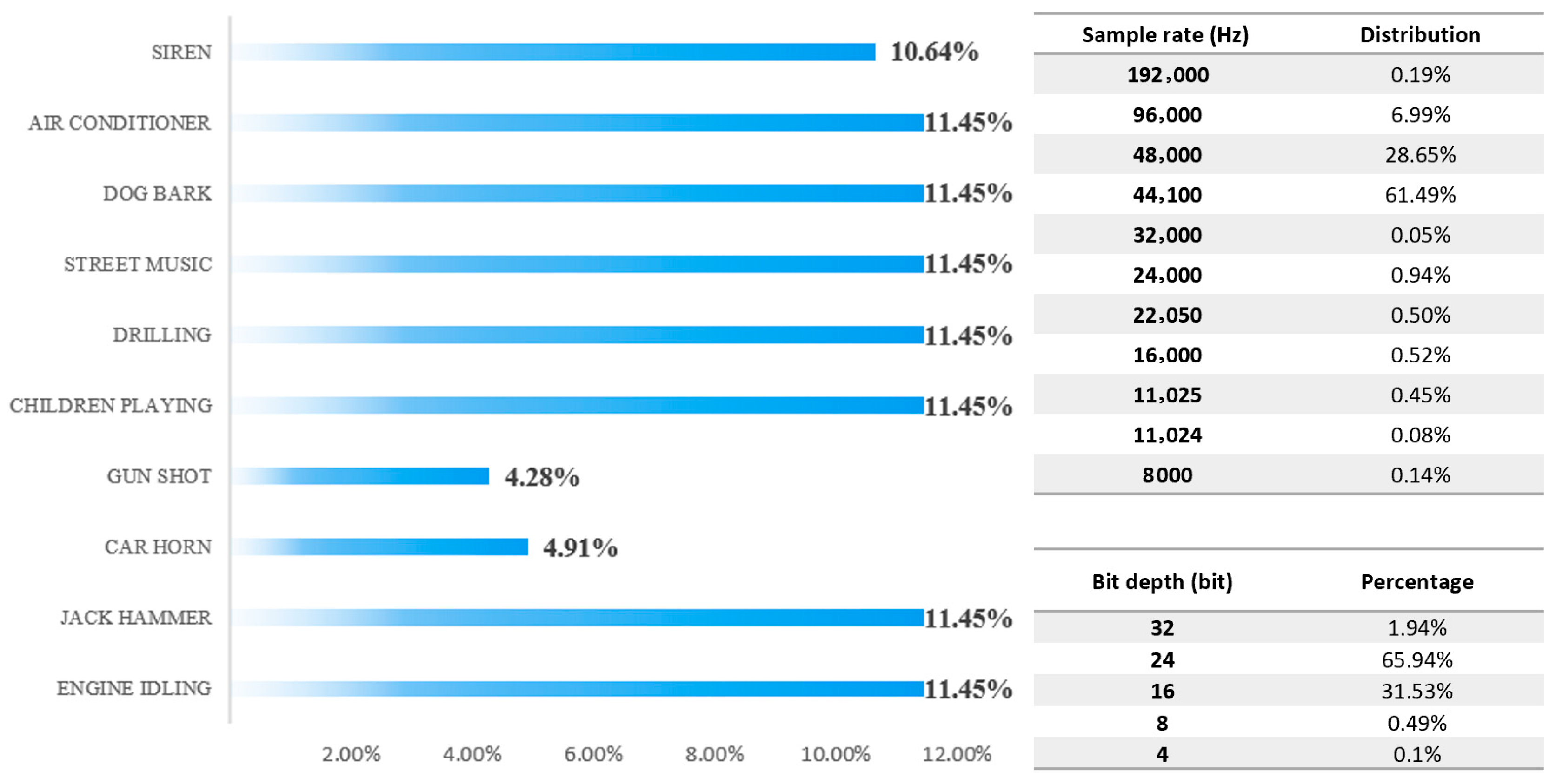
Analysis of the database has been performed, as shown in Figure 2. The dataset shows imbalance across categories, with gunshots and car horns underrepresented. Class imbalance can affect the performance of AED/C, as models may learn biased patterns and achieve lower accuracy for rare events.
From the class distribution analysis, we can see that eight categories have a relatively balanced representation, while two categories—gunshots and car horns—have lower representation, with less than 50% of the average of the other classes. The impulsive nature of these two classes would allow easier detection. The imbalance of the database may lead to lower recognition accuracy. To mitigate this effect during model training, class weighting was applied in the loss function to give higher importance to underrepresented classes, ensuring that the models do not become biased toward majority classes. No synthetic data augmentation was applied.
The audio properties, including number of channels, sampling rate, bit depth and time duration, were analyzed to ensure proper feature extraction. The results showed significant heterogeneity in approximately 91.5% of the samples, and approximately 90% of samples were recorded at 44.1 or 48 kHz, representing standard high-quality playback resolution. The audio files were processed, converting them to mono channel without losing information. The lower quality samples were less than 3% of the total, but were kept, so variability was introduced and overfitting in the model training was reduced.
The bit depth analysis indicated values ranging from 4-bit to 32-bit, with the majority (65.9%) recorded at 16-bit, suitable for playback-quality audio. Very low-resolution signals (8-bit or less) were rare (<1%) but still needed normalization. Similarly, the analysis of time duration showed that 85.5% of the audio files last between 3 and 4 s. The other samples were preprocessed with zero padding to achieve a uniform length.
As there is a wide variation in signal properties, normalization is an important step, in order to avoid overpowering, misinterpretation and reduced classification accuracy. To address this, all audio samples were standardized by resampling them at 22.05 kHz with a 16-bit depth, normalizing their amplitude, converting them to mono, and ensuring consistent duration through zero padding. This process retains the frequency range important for urban acoustic events (below 11 kHz, according to Nyquist’s theorem), while simultaneously providing the resolution needed for accurate classification based on machine learning.
In summary, the analysis of the UrbanSound8K database revealed key challenges related to class imbalance, signal heterogeneity, and data quality. The preprocessing steps ensured compatibility in feature extraction and improved the robustness of the ML algorithms.

2.3. Feature Extraction

Audio parameterization of sound events enables the extraction of key features that support high-accuracy classification. Since more than 50 parameters across six domains can be used [64,65,66], the five parameters were selected as they have shown good performance in [13,14].
In order to be able to convert the audio signal using feature extraction, first the audio signals of the sound from the database will be displayed in WAV format as a signal with continuous time interval t N   [ s ] :
x c t               0   t N 4
The continuous signal is processed into discrete signals through the relation
x n = x c n T         < n <
Using the sample rate f s = 22,050   H z , the sample time is T = 0.045   m s . As the audio signal has a duration of t N =   4   s , the signal in discrete time has N = f s · t = 88,200 samples:
x n R 88,200
The discrete signal is framed into windows ( w ) using the Hann window function with a length of w f = 100   m s with overlapping at w p = 50   m s . From here, the signal X [ n ] is a product of the discrete signal and the length of the frame:
X n = x [ n ] · w t
As a result of dividing the signal into time windows, a three-dimensional matrix is obtained in the following form:
X [ n ] R 2205   ×   1103   ×   78
For one frame, the signal has the following form:
{ X n } w R 2205   ×   1103           1     w 78
Furthermore, according to the used audio parameter, additional transformations for feature extraction are applied to each parameter as shown in Figure 3.
Spectral Contrast (SC) measures the difference in decibels between harmonic peaks and noise-dominated valleys across octave-scale frequency sub-bands. After applying a Fast Fourier Transform (FFT), the signal is divided into sub-bands, and peak-valley differences are computed and converted into the logarithmic domain. These features are then decorrelated using the Karhunen–Loève Transform (KLT).
Tonal Centroid (TC) captures the dynamic “center of gravity” of musical notes over time. It is derived from a Constant-Q Transform and a chromagram of the 12 semitones, resulting in a six-dimensional vector that reflects harmonic motion.
Chromagram (Ch) maps the energy distribution across the 12 pitch classes in an octave, providing a perceptual measure of pitch variation. It is computed from the power spectrum and normalized energy values.
Mel Spectrogram (MS) represents the time-frequency structure of the audio signal using the Mel scale, which emphasizes perceptually relevant frequency bands. In this study, 128 Mel coefficients were extracted.
Mel Frequency Cepstral Coefficients (MFCCs) model the perceptual characteristics of sound by applying FFT, Mel filtering, logarithmic scaling, and a Discrete Cosine Transform, where 40 MFCCs were extracted.
MFCCs are widely used for their effectiveness in modeling the perceptual aspects of human hearing, particularly timbral texture. Mel Spectrograms provide a time-frequency representation aligned with the Mel scale, enhancing resolution in lower frequencies, where many urban sounds occur. Chromagrams capture harmonic and pitch content, which is useful for distinguishing tonal events such as music or sirens. Tonal Centroid features represent harmonic relations and are effective for identifying tonal shifts. Spectral Contrast highlights the difference between spectral peaks and valleys, aiding in the discrimination of noisy versus tonal sounds. Together, these features offer a robust multidimensional representation of complex urban audio environments, improving classifier performance across diverse sound classes.
All stages of data processing, feature extraction, model training, and evaluation were performed using Python version 3.9.0. All features were extracted using the Librosa library [67]. The feature extraction process visually shows the extracted parameters of each audio signal and, furthermore, creates a feature vector that is used for training and testing the ML algorithms. Visualization was handled using Matplotlib version 3.3.3 [68] and IPython.display [69].

2.4. Machine Learning Algorithms

2.4.1. Random Forest

The Random Forest Algorithm, introduced by Breiman [70,71], is based on an ensemble of decision trees created from randomly selected training samples to ensure more stable and accurate predictions. The model aggregates assumptions during the induction phase using randomly selected parameters, as discussed in [72]. Random Forests combine multiple decision trees trained on random subsets of data and features. This ensemble approach reduces overfitting and improves prediction robustness, especially in noisy datasets. A dataset D of n samples can be defined as follows:
D = { x 1 , y 1 ,   x n , y n }
where each input sample x i is represented as a feature vector:
x i = ( x i 1 , , x i d )
and the output corresponds to the class y i .
In a decision tree, each node performs a binary split ( x i > a ) based on a selected feature. The splitting is determined using the Gini criterion:
g x i = i = 1 n ( P ^ ( C k | x i ) ( 1 P ^ C k x i )
where the probability that sample x i belongs to class C k is given as follows:
P ^ ( C k | x i ) = | x i C k | | x i |
By randomly generating feature vectors
X = ( X 1 , , X d )
a new dataset D is formed, on which multiple decision trees are trained with randomly selected features, which are obtained randomly through the probability distribution of the features x i , y i ~ ( X , Y ) :
h = { h 1 X , , h k ( X ) }
Each tree is defined by a set of parameters:
λ k = λ k 1 , , λ k p
So the decision function of a single tree can be written as follows:
h k X = h ( X | λ k )
The final classification is obtained by majority voting across all trees. The margin function is defined as follows:
m ^ X , y = P ^ k h k X = y max j y P ^ k h k X = j
And the generalization error is
e = P X , y ( m ^ X , y < 0 )
The calculation of accuracy in the final classification, f ( X ) , depends on the class decision to which a given data point X belongs according to each decision tree, expressed as follows:
f X = k = 1 K 1 K h k ( x )
After training, the predictions of the samples, f ^ , are obtained through the average predictions from all individual decision trees:
f ^ = 1 M m = 1 M f ^ B ( h k )
The algorithm is first trained on a dataset with known class labels, and afterwards tested on an independent dataset, where the class characteristics are already defined, thus allowing the performance of the model to be validated.
The main advantage of Random Forests is their robustness to noisy data, as they can successfully classify signals even when classes are not clearly separated. Moreover, the computational complexity is lower compared to SVM.

2.4.2. Support Vector Machines

The effectiveness of the SVM algorithm depends on the choice of kernel function, which is determined by the data type and its distribution in space [73,74,75]. The database is represented with a p-dimensional vector, while the classes are separated by a (p − 1)-dimensional hyperplane. For a dataset D, consisting of n samples, the training set is defined as follows:
D = x i , y i x i R p ,   y i 1,1 n i = 1
To find the separating hyperplane with maximum margin, consider the normal vector w of the hyperplane that separates the classes y i , where y i = 1 or y i = 1 . The hyperplane can then be expressed as follows:
w · x b = 0
If the data is linearly separable, two supporting hyperplanes (margins) can be introduced:
w · x b = 1
w · x b = 1
The margin between them is 2 w . To maximize the margin, the scalar w must be minimized under the following condition:
y i ( w · x i b ) 1 ,           1 i n
This leads to the optimization problem:
a r g   min ( w , b ) 1 2 w 2
Using Lagrange multipliers α , the constrained problem becomes
a r g   min ( w , b )   max α 0 { 1 2 w 2 i = 1 n α i [ y i w · x i b 1 ] }  
By applying Karush–Kuhn–Tucker (KKT) conditions, the solution can be expressed as follows:
w = i = 1 n α i y i x i
i = 1 n α i y i = 0
Only support vectors satisfy the condition:
y i w · x i b = 1
With the introduction of the average value of the support vectors N S V , the bias b can then be computed as follows:
b = 1 N S V i = 1 N S V w · x i y i
The dual optimization problem reduces to
a r g   min ( w , b )   max α 0 { i = 1 n α i 1 2 i = 1 n j = 1 n α i α j y i y j x i x j }  
Here, the dot product x i x j , can be replaced by a kernel function f x = k x i , x j . Thus, SVM algorithms use kernel functions to transform the input data into higher-dimensional space, enabling better class separation.

2.4.3. Naive Bayes

Naive Bayes classifiers apply Bayes’ theorem under the assumption that features are conditionally independent [76,77]. Despite this simplification, they are widely used because they scale well to large datasets and are computationally efficient [78].
A data instance x consisting of n independent features can be represented as follows:
x = ( x 1 ,   ,   x n )
For each class C k , the posterior probability is
p ( C k | x ) = ( C k x 1 ,   ,   x n )
Applying Bayes’ theorem, this becomes
p C k x = p C k p x C k p x
Here, p C k x is prior, p x C k is the likelihood, and p x is the evidence. Since the denominator is constant across classes, classification depends on the numerator, equivalent to the joint probability:
p = ( C k , x 1 ,   ,   x n )
Expanding with the chain rule of probability,
p ( C k , x 1 ,   ,   x n ) = p C k p x 1 ,   ,   x n C k = p C k p x 1 C k p x 2 ,   ,   x n C k , x 1 = p C k p x 1 C k p x 2 C k ,   x 1 p x n C k , x 1 ,   x 2 x n 1
Using the Naive conditional independence assumption, where each feature x i is independent of all others given C k ,
p x i C k , x j = p x i C k                                             з a         i   j
This reduces the joint probability to
p = C k x 1 ,   ,   x n   p C k i = 1 n p x i C k
Normalizing by the evidence Z   =   p ( x ) , the conditional distribution is
p C k x 1 ,   ,   x n = 1 Z p C k i = 1 n p x i C k
Finally, the classifier assigns the most probable class using the decision rule:
y ^ = argmax k { 1 , , K } p C k i = 1 n p x i C k
The decision is given to the class with the highest posterior probability. Parameter estimation can be achieved either by assuming a specific distribution (e.g., Gaussian, multinomial) or by generating probability models from the training data.

2.4.4. Hyperparametrization

Hyperparameter Optimization (HPO) achieves high performance from ML algorithms by selecting the best set of parameters for each model. The appropriate choice of hyperparameters directly influences model accuracy. HPO may involve continuous or discrete parameters and requires a good understanding of both the algorithm and the optimization method [79,80,81].
Let a machine learning model A , an HPO algorithm H and a dataset D be given. The training dataset D t r is used to optimize hyperparameters, while D t is used for testing. The model on training data is defined as follows:
f A , D t r = A ( D t r )
With expected loss L ,
L ( D t r , f A , D t r )
Hyperparameters λ = λ 1 ,   ,   λ n define the model configuration:
f λ = f ( A λ ,   D t r )
The hyperparameter space λ contains all candidate values. HPO requests the λ * minimizing the expected loss of test data:
Φ A , D :   Λ         [ 0 ,   1 ] λ     m e a n D t L ( D t , f A λ , D t r ) λ * = min λ ( m e a n D t L ( D t , f A λ , D t r ) )
HPO methods use gradient descent for continuous parameters and Bayesian optimization or decision approaches for discrete ones. Model-based optimization, including the Gaussian Process optimization, uses the hyperparameter space to achieve maximum predictive accuracy while balancing computational complexity.
The main goal is to identify hyperparameters λ * that produce the most accurate model for test data, ensuring high performance across different machine learning algorithms.

2.5. Convolutional Neural Networks

Convolutional Neural Networks are specialized architectures used for processing data with grid-like topology, particularly effective in image processing and classification. Deep learning uses datasets for training and testing to predict outcomes, often applied in pattern recognition and big data scenarios [82]. The input data used for training and testing CNNs are typically three-dimensional vectors, i.e., third-order tensors, representing images of dimensions, where H is the number of rows, W is the number of columns, and D is the number of channels:
x i L l = 1   R H i   ×   W i   ×   D i                                                     1 i n  
CNNs process data through sequential layers: convolution (feature extraction), activation (nonlinearity), pooling (dimensionality reduction), and fully connected layers (classification) [83]. The model learns by minimizing loss via gradient descent [84]. The predicted class is obtained using the maximum output probability [85]. These mechanisms make CNNs highly effective for image recognition and classification tasks. The CNNs consist of multiple processing layers w l :
w l L l = 1
The general structure can be shown by the expression
x 1     w 1 x 2   x L 1   w L 1 x L   w L z  
The final output x L belongs to possible classes C :
x L R C
Classification is achieved by choosing the class with maximum probability:
arg max l   x i L
Loss factor and Optimization
To measure prediction error, CNNs use a loss function. For a target t , the squared error is
z = 1 2 t x L 2
Training updates of the parameters are established using Stochastic Gradient Descent (SGD):
w l w i η z w l
In Expression (4), the sign implicitly indicates that the parameters w l of the l th layer are updated from time t to t + 1 . If the time index t is used explicitly,
( w l ) t + 1 = ( w l ) t η z ( w l ) t
The learning rate must satisfy the rate of learning η :
η 1
Activation function
After convolution, nonlinearity is introduced using the Rectified Linear Unit (ReLU):
y i , j , d = max { 0 , x i , j , d l }
ReLU outputs positive values or zero, enhancing feature discrimination.
Convolutional layer
Given input tensor x l     H l   ×   W l   ×   D l and kernels, convolution reduces dimensionality while extracting spatial features. The vectorized operation is
v e c y = v e c ( x l + 1 ) = v e c ( φ ( x l ) F )
with
F R H W D l × D
The gradient for updating kernels is
z F = φ ( x l ) T z Y
Pooling layer
Pooling reduces spatial dimensions and computation:
H l + 1 = H l H         W l + 1 = W l W       D l + 1 = D l
The maximum pooling method used in this study is
y i l + 1 , j l + 1 , d = max 0 i < H , 0 j < W x i l + 1   ×   H + i , j l + 1   ×   W + j , d l
ADAM algorithm
CNN training was optimized using the ADAM algorithm [86], which adaptively adjusts learning rates for each parameter by combining the benefits of AdaGrad [87] and RMSProp [88]. The implementation method of this algorithm is computationally efficient and is used for non-stationary problems with gradients that are not well-defined and contain a lot of noise [89].
These mathematical formulations inform the design of our CNN architecture, which is detailed in the following Section 3.2. The CNN architecture was designed to balance feature richness and computational efficiency. A 2 × 2 kernel size was selected to preserve fine-grained spatial patterns while reducing parameter count. The progressive increase in filter depth (from 16 to 128) allows hierarchical feature extraction, capturing both low-level and high-level acoustic patterns. A dropout rate of 0.2 was empirically chosen to mitigate overfitting without significantly impairing learning capacity. The depth of four convolutional layers was found to be optimal during validation, offering sufficient abstraction without excessive complexity.

3. Results

3.1. Classic Machine Learning Algorithms

3.1.1. Results from Testing 48 Different Models for Feature Vectors and ML Algorithms

By combining the five audio parameters and the three ML algorithms, a total number of 48 models were trained and tested to see performance for accuracy in classification. A comparison of results was performed and the model with the highest accuracy is chosen for further optimization. To ensure the reliability and generalizability of the reported results, each model configuration was evaluated using 10-fold cross-validation, and the mean accuracy and standard deviation across folds are presented in Table 1. This statistical dispersion provides insight into the consistency of each model’s performance and supports the comparative analysis of feature combinations and classifier behavior. The inclusion of standard deviation values substantiates the observed accuracy differences and reinforces the robustness of the selected feature sets.
Mel Frequency Cepstral Coefficients (MFCCs) are used as fundamental parameters for recognizing and classifying sound events due to their ability to capture perceptually relevant frequency characteristics, which improves model accuracy. To determine the optimal number of Mel filter banks, we tested a range from 10 to 40 coefficients (10, 20, 30 and 40). The highest classification accuracy for all three machine learning algorithms was achieved using 40 coefficients, which provides sufficient frequency resolution to capture the spectral characteristics of urban acoustic events in the UrbanSound8K dataset, while avoiding excessive computational complexity.
In the next phase of testing, the MFCCs are retained, and another parameter is added to them. An analysis is performed to evaluate how the addition of each parameter affects system accuracy, and the results are presented in the table. From the results, it can be seen that the Mel Spectrogram (MS) decreases the accuracy of the tested data in all three algorithms. This decrease is especially noticeable in the Naive Bayes algorithm, where the accuracy is reduced by 21.39% compared to using the MFCC parameter alone—almost half of its value. The RF and SVM algorithms also show decreases of 8.12% and 0.87%, respectively.
When testing the system using the MFCC and Spectral Contrast (SC) parameters, the accuracy of the RF algorithm improves by 2.15%, while the accuracy achieved in the other models decreases. The combination of Chromagram (CH) and Spectral Contrast parameters leads to an increase in accuracy when testing the system. The highest accuracy for the SVM algorithm (64.04%) is achieved by applying the audio parameters MFCC and Chromagram while, for the RF and NB algorithms, the highest accuracies are achieved when combining the MFCC and Spectral Contrast parameters (58.78% for RF and 50.53% for NB).
In the next phase, combinations of more than two parameters are tested to determine whether recognition and classification accuracy can be improved. It is observed that the highest accuracy for all three ML algorithms is achieved when extracting Mel Frequency Cepstral Coefficients, Chromagram, and Spectral Contrast. When using these three parameters, a total of 59 coefficients are applied: 40 for MFCC, 12 for Chromagram, and 7 for Spectral Contrast. These 59 coefficients are extracted to form the feature vector, which is then used as the input parameter for the ML algorithms. It is also noted that the Mel Spectrogram and Tonal Centroid parameters reduce the accuracy of the model.
Next, four parameters are combined, keeping the base 40 parameters of MFCC in each variant, from which four different feature vector combinations are obtained. From the results, it can be concluded that accuracy decreases when using the Mel Spectrogram in combination with the other parameters. Although the Mel Spectrogram is known to achieve promising results when using deep learning techniques, the results shown in the table confirm that this parameter significantly reduces the accuracy when using these three algorithms. Even when applying all five parameters, which extract 193 coefficients for each audio signal, it can be noted that the accuracy of the model is still lower than the accuracy obtained when applying the three mentioned features. The feature extraction for each audio file required approximately 0.8–1.2 s per file; training time for classical ML models ranged from 2 to 5 min depending on complexity.
For classification tasks, models were implemented using scikit-learn [90] and TensorFlow/Keras [91], respectively. Hyperparameter tuning was conducted using grid search. Additional utilities such as pandas and numpy were used for data handling, while the Python struct module supported low-level parsing of WAV file headers. All toolkits used are well-established and widely validated in the machine learning and audio signal processing communities, ensuring methodological robustness and reproducibility.

3.1.2. Applying Hyperparameter Optimization

Hyperparameter optimization was further applied in order to increase the accuracy to the three algorithms using MFCC, Spectral Contrast, and Chromagram, as this combination demonstrated the highest accuracy among all tested models.
Hyperparameter optimization for all three classifiers was conducted using grid search, allowing systematic exploration of parameter combinations. For the Random Forest model, the search space included number of estimators values of [100, 500, 1000, 1500], and maximum depth values of [30, 40, 50, 60], with minimum samples per leaf [1, 2, 5] based on validation performance. For the SVM model, the grid search explored C values [1, 10, 20, 30], and gamma values [1 × 10⁻³, 1 × 10⁻⁴, 1 × 10⁻⁵], using an RBF kernel. The Naive Bayes classifier was optimized by tuning the variable smoothing parameter which controls stability in GaussianNB model in the range [1 × 10⁻⁹, 1 × 10⁻⁸, 1 × 10⁻⁷, 1 × 10⁻⁶], and applying feature selection to retain the top 40 features based on mutual information scores. These optimization strategies ensured that each model was evaluated under its most favorable configuration, enhancing the reliability of the comparative results.
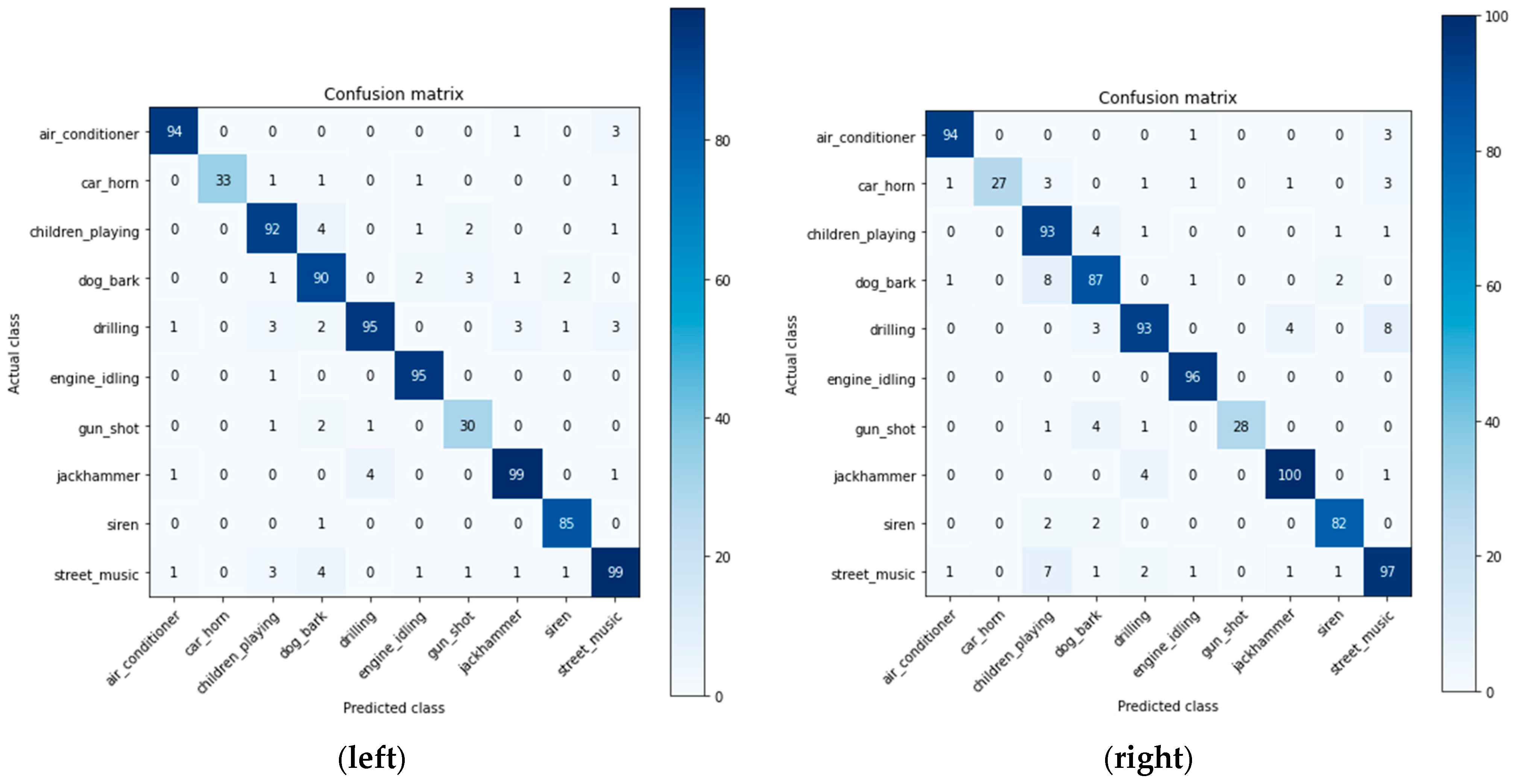
After the optimization, accuracy of 92.9% was obtained for the SVM algorithm, 91.53% for the RF algorithm and 53.68% for the NB algorithm. For the RF, the number of estimators refers to the number of trees in the algorithm, with a default value of 100, while 1500 estimators were selected based on optimization. The maximum depth, set to 60, defines the extent of tree splitting, the minimum number of leaves was optimized to 1, and other parameters (such as decision criterion, maximum number of features, and maximum number of samples) were kept at their default values, as they are not expected to significantly affect the data classification. The application of HPO in the SVM algorithm improves classification accuracy by tuning three parameters: the regularization parameter C, the kernel coefficient, and the gamma coefficient. Based on optimization, the selected values were C = 30, gamma = 0.0001, and a radial basis function (RBF) kernel. The NB algorithm has not shown good results in classification, so it will not be used for further analysis. Figure 4 shows the confusion matrices of the SVM and RF algorithm. From the applied methodology, it can be noticed that a key role in building a successful system for recognition and classification of sound events has a choice of audio parameters, as well as a choice of machine learning algorithms and the applied hyperparameter optimization.
From the results, it can be noticed that the most accurately predicted class is the class representing engine idling, where only one class was wrongly predicted. The sound of a siren and of air conditioning are events that have few errors in the process of classification. The biggest prediction errors in all three algorithms occur for the same classes: drilling and street music. When analyzing sound events, it can be seen that the sound class that represents music contains many elements, and each piece of data that represents this class has a different visual representation. In the sound class representing drilling, low-frequency sounds appear and the drilling sound itself contains a lot of noise, which is probably the reason for the error while predicting the data. This consistent misclassification across all confusion matrices suggests that the error likely originates during feature extraction rather than from the machine learning algorithms themselves.

3.2. Results from Testing CNN

Convolutional neural networks are developed as algorithms that have undergone significant development in the field of deep learning and artificial intelligence in recent decades due to the high efficiency of their application. A theoretical review of modeling algorithms for convolutional neural networks is given in order to develop a mathematical model of the algorithm that will be used for recognition and classification. The developed algorithm is implemented using four different feature vectors, resulting in the development of four algorithms for convolutional neural networks. When testing the algorithms, two models showed excellent performance achieving accuracy higher than 90%.
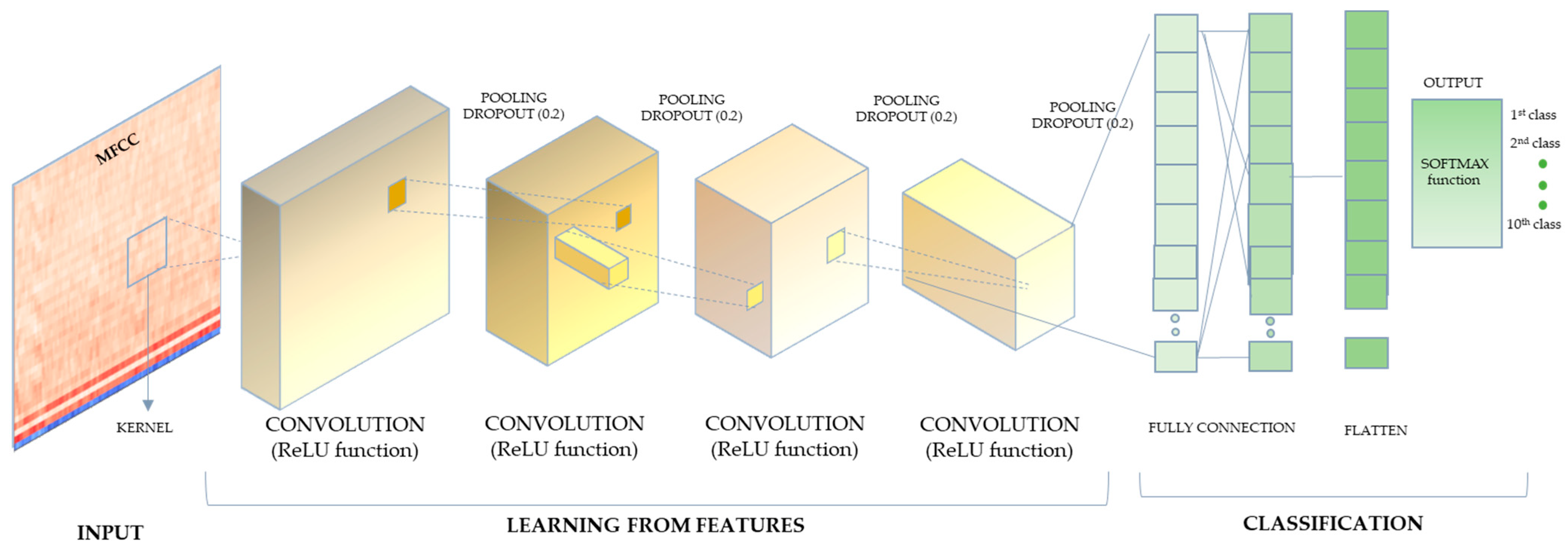
After training and testing the system, it can be concluded that the most successful model is CNN, which uses Mel frequency cepstral coefficients with an accuracy of 97.95% in the train phase and 92.68% in the test phase. The structure of the CNN is shown in Figure 5 and Table 2, where four convolutional layers are used. The number of filters varies from 16 to 128, starting from a smaller number of filters for the first layer to 128 filters for the last convolution layer. According to research, the number of filters should be increased when applying more convolutional layers. ReLU activation function is used in all filters. Due to the large amount of data, the dropout function is applied in order to reduce the data. After each convolutional network, the dropout coefficient is 0.2. After the convolution, a global average pooling and flattening is applied, followed by final classification layer using the SOFTMAX function. The total numbers of used parameters in the convolutional layers and the last classification layer is 44,602. The dimensions of the input data are (40, 174).
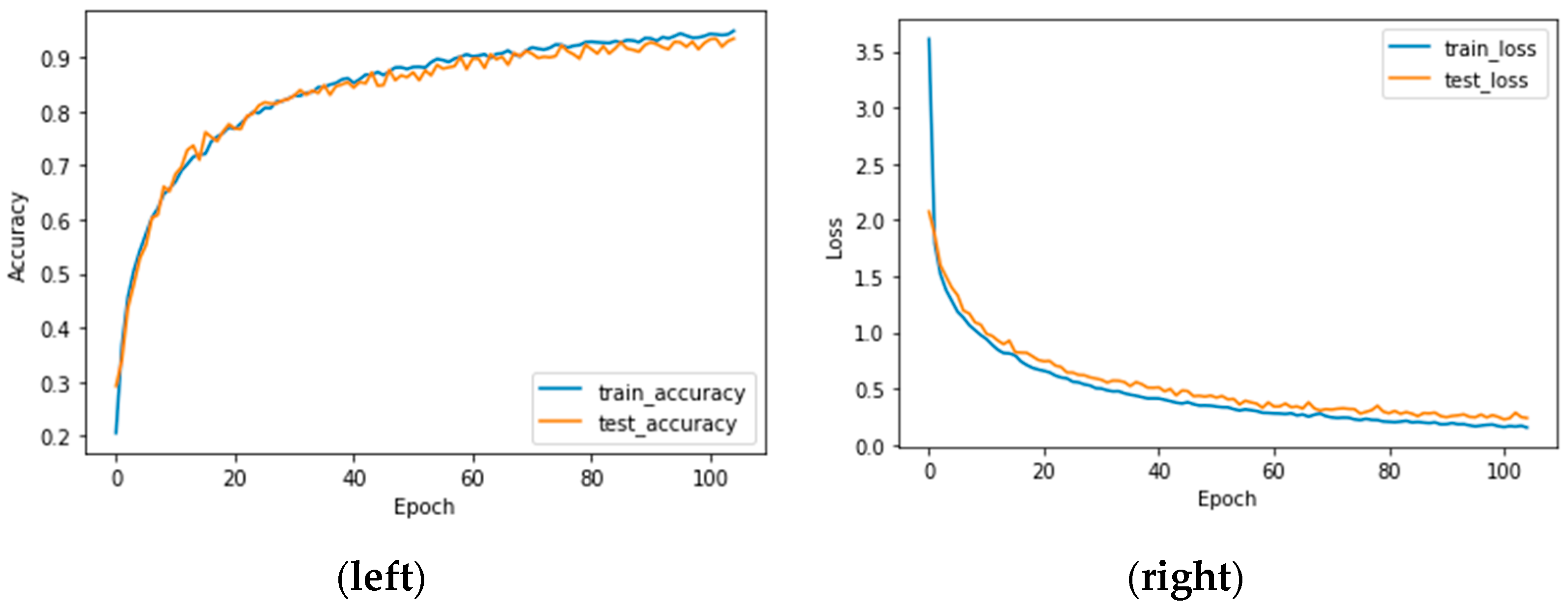
The model was trained for 50 epochs with a batch size of 32, using the Adam optimizer and categorical cross-entropy loss. Convergence was monitored using validation accuracy, and early stopping was applied with a patience of five epochs to prevent overfitting. Training duration averaged 12 min per fold on a standard GPU setup. These settings were selected based on empirical validation to balance learning efficiency.
The results for accuracy and the loss curve are shown on Figure 6, from where it can be noticed that the accuracy achieved during testing is higher than the accuracy during training. This is normal because not all characteristics are used during training (according to the dropout function), while all features are used for the testing phase. The same case occurs for the loss curve, from which it can be seen that the loss while testing is less than the loss while training the CNN. The curves follow a gentle path and there is no overlap, which is a good sign when designing the architecture of CNN.
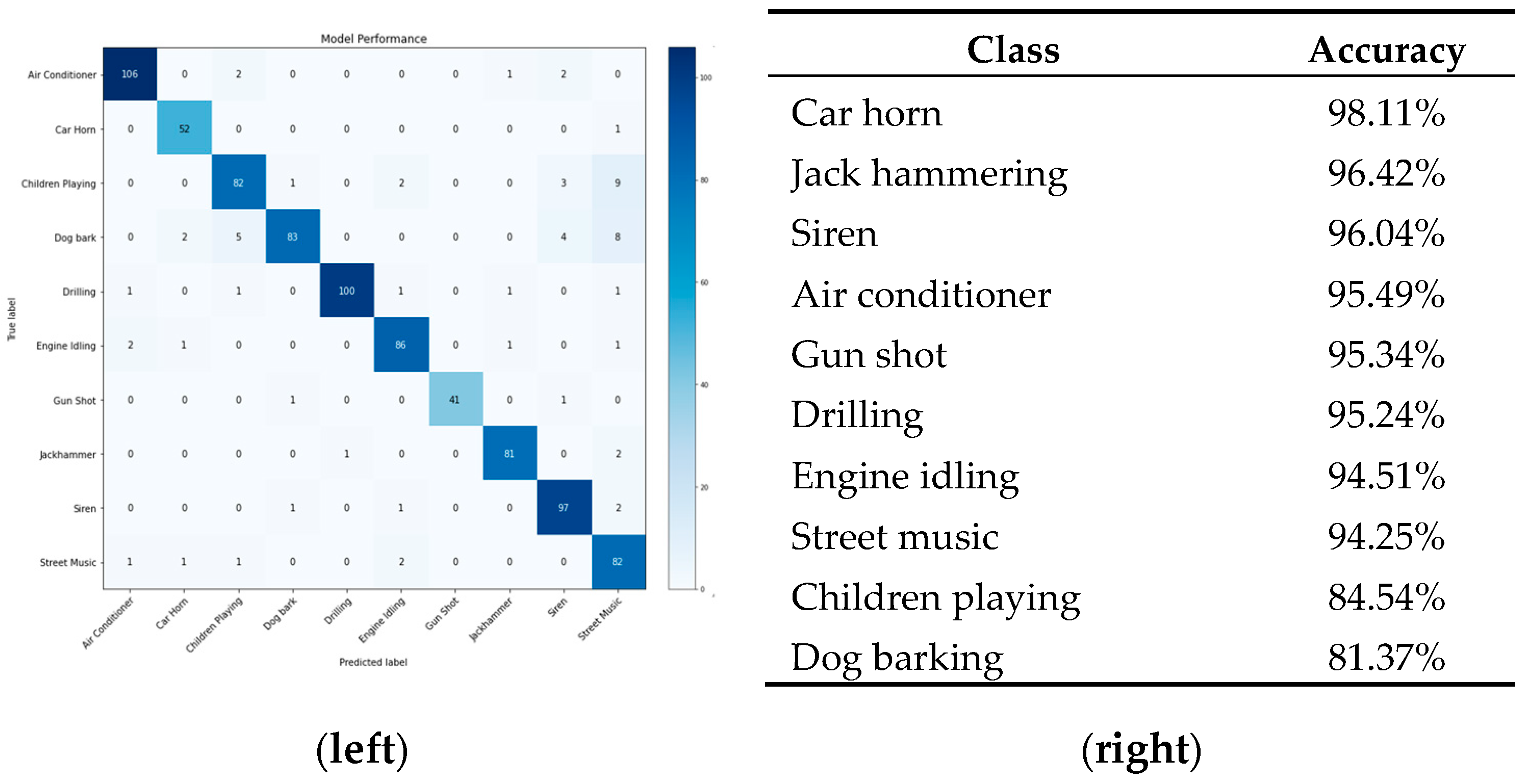
According to the confusion matrix analysis, shown in Figure 7, the table on the right shows the percentage accuracy for each class separately. It can be noticed that the major error occurs in the classes children playing in the street (84.53%) and dogs barking (81.37%), and the highest uncertainty is for street music. The most precise prediction is for car horn, with an accuracy of 98.11%.
When listening to the sounds from the database, clear signs of poor classification performance can be observed when the target sound is not distinct enough and additional sound sources are present in the audio data. The fact that this happens often in this database makes it difficult to distinguish between some classes, which may be the reason for the lower accuracy.
Modeling using deep learning techniques has an advantage over the classic machine learning algorithms if the system to be modeled is complex and needs to be applied in real-time applications. Since the difference between the achieved accuracy of the most successful models is very small (0.22%), the model composed of MFCC as audio parameter and the CNN as algorithm that uses artificial intelligence techniques will be used for further validation by testing the system with data outside the database.

3.3. Real-Time Validation and Application on Real System

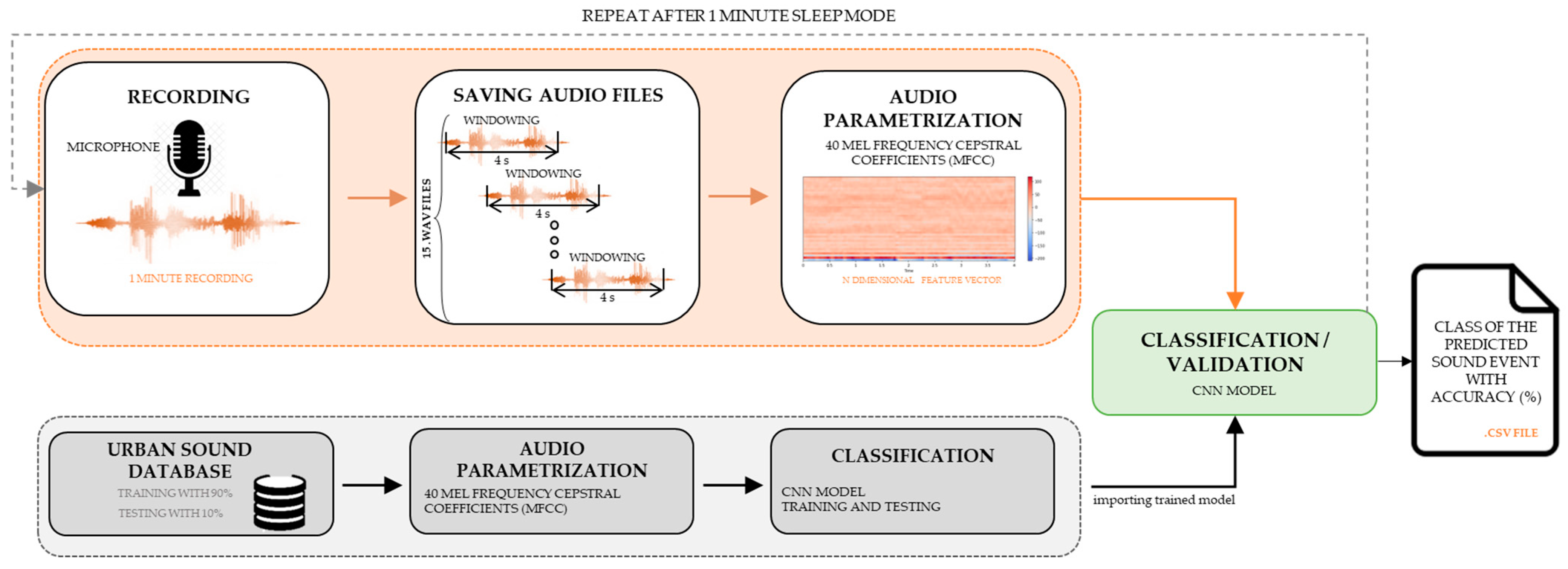
Validation of a system based on artificial intelligence involves testing of the trained system with unknown data from an independent database. The purpose of validation is to measure the performance of the system when implementing it in a real application. The validation process was conducted in two phases. The block diagram indicating the steps for validation is shown in Figure 8. The “detection-by-classification” approach was applied for audio event detection, which extracted audio segments of fixed length from a continuous incoming stream. Each recorded audio segment lasted 4 s, which was sufficient to determine the sound class while minimizing latency and computational load. The system recorded 15 audio files, each lasting 4 s and captured at 1-min intervals. This saved the recordings as.WAV files, processed the information, applied parameterization, and used a pretrained ML algorithm to output the predicted sound class for each recording.
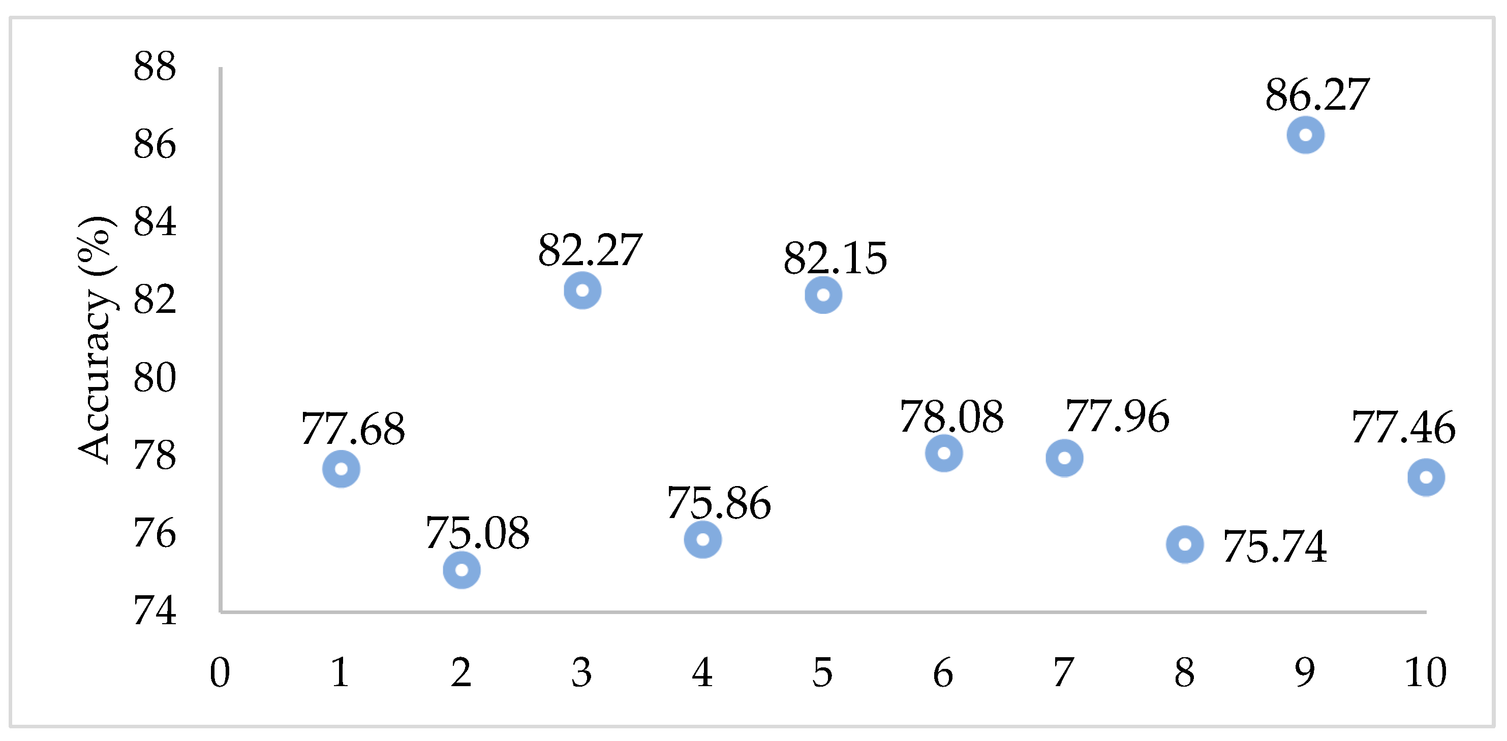
In the first phase of validation, the system was tested with recorded data from the 10 classes of sound events, where this data was unlabeled. In order to compare the accuracy obtained of the system during validation, 10 iterations were made. For each iteration, 100 recorded audio files consisting of the 10 classes of sound event were used. The final result showed the accuracy of the classification and the predicted class. Based on these results, Figure 9 shows the accuracy for each iteration, which varies between 75.86 %   a n d   6.27 % . The average accuracy for the validation results is 78.86 % .
In the second phase, a real-time validation experiment was conducted using the deployed wireless sensor unit (WSU) near the university campus, specifically in a semi-open courtyard adjacent to a pedestrian walkway and a street. The recording algorithm captured 15 min of ambient sound, segmented into 4-s intervals, resulting in a total of 225 audio samples. The real-time validation was performed on these representative samples to confirm the feasibility of deployment and assess latency performance on the IoT device, rather than for full statistical generalization. The microphone (MEMS type, omnidirectional) as shown in fourth section of the paper, was positioned approximately 1.2 m above ground level and 3 m from the nearest building wall. Environmental conditions included moderate foot traffic, occasional vehicle movement, dogs barking and people talking. The classification accuracy for this phase ranged from 42.86% to 85.71%, with lower accuracy attributed to residual noise or sound events not belonging to the predefined classes. These were frequently misclassified as air conditioning due to spectral similarity. This setup reflects realistic deployment conditions and supports the feasibility of the system in uncontrolled urban environments.

4. Discussion

The theoretical analysis of feature extraction and AI modeling provided clearer insights during the development of the AED/C systems. Using different combinations, 52 classical ML models and four CNN models were experimentally analyzed to develop a system with high prediction accuracy. The best-performing model, based on MFCC features and a CNN architecture, was further validated to assess its applicability and identify potential improvements. The validation revealed that sound events containing residual noise were often misclassified as air conditioning. Since the algorithm is intended for stationary wireless sensor units (WSUs) in urban areas, this class was renamed as “residual noise”. This modification reflects a broader ontology refinement, grouping low-intensity or background urban sounds that do not correspond to distinct acoustic events. Additionally, results with accuracy below 60% were excluded to ensure reliable classification outcomes.
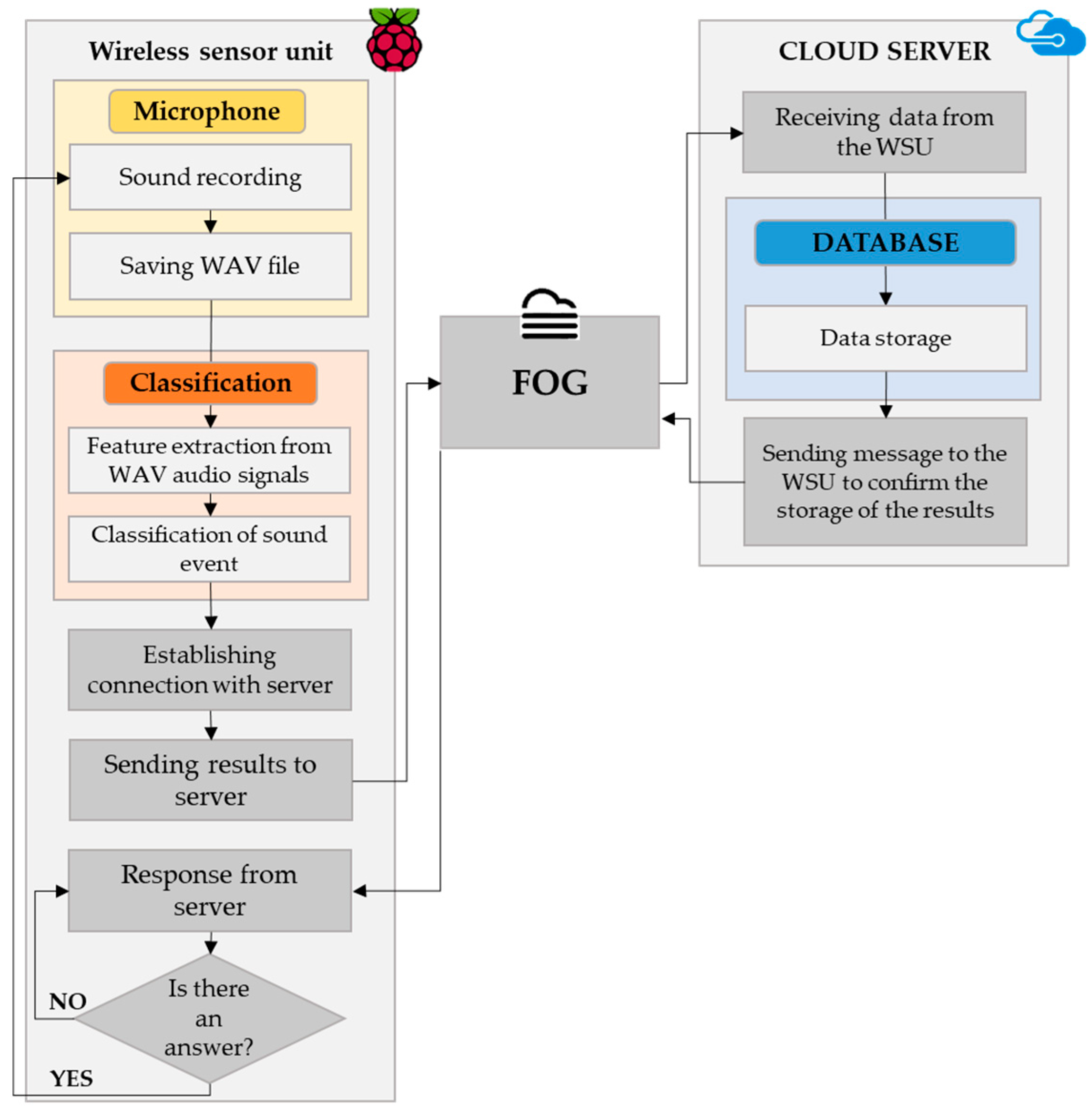
To design the WSU, a logical flow is presented in Figure 10. Specifically, the system architecture follows a fog-to-cloud model, where each wireless sensor unit (WSU) performs local classification using a pretrained CNN and transmits the results via Wi-Fi to a cloud server (Google Drive) through a fog-layer router.
At the core of IoT-based applications is a cloud server for data storage and processing. Integrating cloud and fog computing enables the implementation of algorithms for image processing, translation, and sound classification. Fog analytics support local decision-making, while cloud analytics process data from larger regions, allowing deeper abstraction as information travels through the smart city infrastructure. The dynamic nature of smart cities requires advanced AI and machine learning algorithms that can adapt to real-time conditions. Embedding intelligent mechatronic systems with AI ensures high data availability and delivers actionable insights for the population. With multiple WSUs deployed across urban areas, smart city implementations become more reliable.
For acoustic event detection, WSUs should be installed in the noisiest urban locations. Each unit consists of a low-cost microcontroller with an integrated algorithm and a microphone. After classification, the results are transmitted through the fog network to the cloud server, where they become accessible to end users.
Based on this, the hardware components for the WSU were selected to ensure low cost and accessibility for implementing the constructed AED/C system. The WSU can be seen in Figure 11, consisting of microcontroller, microphone and external battery→, as well as box and cables, with a total cost of around EUR 110. The UrbanSound8K used for training and testing the system is 8 GB. The CNN and feature extraction require high processing power and large memory.
At the core of the system is a Raspberry Pi, which features a quad-core ARM Cortex A53 processor running at 1.2 GHz, with about 350 mA with 4 GB SDRAM, a 64 GB memory card, built-in WiFi, and low power consumption. CNN training requires approximately 12 min per model on a quad-core Raspberry Pi. Classification time per audio segment was under 1 s. These timings reflect the performance on the actual deployment platform and support the feasibility of near real-time classification in low-resource environments. CNN training is performed offline during system development, while real-time classification during deployment occurs within seconds, supporting the one-minute operational cycle.
For cloud integration, the system uses Google Drive as the server. During initial testing, sound is captured using a basic, affordable omnidirectional electret USB microphone with recording at 48,000 Hz and 32-bit depth. After each 1-min recording session, the Raspberry Pi processes the data locally, running a classification script that evaluates the sound and predicts its noise category. Once the analysis is complete and the sound event is classified, the results are automatically uploaded to the cloud server via Wi-Fi using a fog-layer router. The results, stored as csv files, include classification outcomes and achieved accuracy on the cloud server via Google Drive. These can later be visualized to highlight the areas with the most noise pollution and identify the type of sound pollution recorded.
In the context of M2M (machine-to-machine) communication, the term real-time denotes the system’s capability to perform audio event detection and classification within a one-minute operational cycle. Specifically, the WSU records 15 audio segments, each lasting 4 s, and then enters a low-power mode while locally processing the data using a pretrained machine learning algorithm. The classification results are subsequently transmitted to the cloud. This operational cycle ensures that each sound event is captured, analyzed, and communicated within the same minute, providing timely responsiveness suitable for urban noise monitoring and smart city applications.
Future research will focus on installing multiple WSUs to help reduce urban noise pollution. AED/C systems are vital in many engineering fields, and their importance continues to grow with advances in real-time data processing.

5. Conclusions

The study confirmed that advanced methodologies for acoustic event detection and classification can significantly enhance the monitoring of noise pollution in urban areas. Standard approaches, although accurate, are limited in capturing the full range of influential noise sources. By selecting five key audio parameters and applying machine learning algorithms, a comprehensive experimental analysis was conducted, resulting in models with competitive prediction accuracy, from which one model was chosen and further validated with unknown sound events.
The integration of IoT, cloud, and fog computing creates a scalable framework capable of processing, storing, and analyzing sound data in real time. This architecture ensures both local decision-making and broader city-level management. The implementation of WSUs based on a Raspberry Pi microcontroller combined with digital microphone, proved to be an efficient, low-cost, and energy-saving solution for real-time classification of urban sounds.
The findings highlight the applicability of these systems within smart city infrastructures, enabling continuous noise monitoring and better environmental management. Future work will focus on large-scale deployment of WSUs and further optimization of algorithms to reduce urban noise pollution and strengthen sustainable urban development. Ultimately, such systems can improve public health, well-being, and the overall quality of urban life.

Author Contributions

Conceptualization, S.D.M.; methodology, S.D.M.; software, S.D.M. and D.P.; validation, S.D.M. and D.P.; formal analysis, S.D.M. and V.G.; investigation, S.D.M. and M.A.; resources, S.D.M. and M.A.; data curation, D.S. and A.A.I.; writing—original draft preparation, S.D.M.; writing—review and editing, S.D.M., V.G. and M.A.; visualization, S.D.M.; supervision, V.G.; funding acquisition, S.D.M. All authors have read and agreed to the published version of the manuscript.

Funding

This research and the APC was funded by the Ministry of Education of North Macedonia grant number 505645.

Institutional Review Board Statement

Not applicable

Informed Consent Statement

Not applicable

Data Availability Statement

The original contributions presented in this study are included in the article. Further inquiries can be directed to the corresponding author(s).

Conflicts of Interest

The authors declare no conflicts of interest.

References

  1. European Commission. Green Paper on Future Noise Policy. 1996. Available online: https://op.europa.eu/en/publication-detail/-/publication/8d243fb5-ec92-4eee-aac0-0ab194b9d4f3/language-en (accessed on 10 October 2025).
  2. World Health Organization. The World Health Report: 2003: Shaping the Future. 2003. Available online: https://pmc.ncbi.nlm.nih.gov/articles/PMC313882/ (accessed on 10 October 2025).
  3. Blanes, N.; Fons, J.; Houthuijs, D.; Swart, W.; de la Maza, M.S.; Ramos, M.J.; Castell, N.; van Kempen, E. Noise in Europe 2017: Updated Assessment; European Topic Centre on Air Pollution and Climate Change Mitigation (ETC/ACM): Bilthoven, The Netherlands, 2017. [Google Scholar]
  4. Handbook on the Implementation of EC Environmental Legislation, Section 9—Noise Legislation. Available online: https://op.europa.eu/en/publication-detail/-/publication/2b832b9d-9aea-11e6-868c-01aa75ed71a1 (accessed on 10 October 2025).
  5. World Health Organization. Guidance on Environmental Noise, Report. 2024. Available online: https://www.who.int/tools/compendium-on-health-and-environment/environmental-noise (accessed on 10 October 2025).
  6. Zannin, P.H.T.; Engel, M.S.; Fiedler, P.E.K.; Bunn, F. Characterization of environmental noise based on noise measurements, noise mapping and interviews: A case study at a university campus in Brazil. Cities 2013, 31, 317–327. [Google Scholar] [CrossRef]
  7. Bąkowski, A.; Radziszewski, L.; Dekýš, V.; Šwietlik, P. Frequency analysis of urban traffic noise. In Proceedings of the 2019 20th International Carpathian Control Conference (ICCC), Wieliczka, Poland, 26–29 May 2019; pp. 1–6. [Google Scholar]
  8. Stansfeld, S.A.; Matheson, M.P. Noise pollution: Non-auditory effects on health. Br. Med. Bull. 2003, 68, 243–257. [Google Scholar] [CrossRef]
  9. European Union. Directive END 2002/49/EC of the European Parliament and of the Council of 25 June 2002 Relating to the Assessment and Management of Environmental Noise; European Union: Brussels, Belgium, 2002. [Google Scholar]
  10. ISO 1996-1; Acoustics—Description, Measurement and Assessment of Environmental Noise—Part 1: Basic Quantities and Assessment Procedures. International Organization for Standardization: Geneva, Switzerland, 2016.
  11. ISO 1996-2; Acoustics—Description, Measurement and Assessment of Environmental Noise—Part 2: Determination of Environmental Noise Levels. International Organization for Standardization: Geneva, Switzerland, 2017.
  12. Socoró, J.C.; Sevillano, X.; Alías, F. Analysis and automatic detection of anomalous noise events in real recordings of road traffic noise for the LIFE DYNAMAP project. In Proceedings of the INTER-NOISE and NOISE-CON Congress and Conference Proceedings, Hamburg, Germany, 21–24 August 2016; Institute of Noise Control Engineering: Wakefield, MA, USA, 2016; Volume 253, pp. 1943–1952. [Google Scholar]
  13. Socoró, J.C.; Alías, F.; Alsina, R.M.; Sevillano, X.; Camins, Q. B3-Report Describing the ANED Algorithms for Low and High Computation Capacity Sensors; Report B3; Funitec La Salle: Barcelona, Spain, 2016. [Google Scholar]
  14. Sevillano, X.; Socoró, J.C.; Alías, F.; Bellucci, P.; Peruzzi, L.; Radaelli, S.; Coppi, P.; Nencini, L.; Cerniglia, A.; Bisceglie, A.; et al. DYNAMAP—Development of low cost sensors networks for real time noise mapping. Noise Mapp. 2016, 3, 172–189. [Google Scholar] [CrossRef]
  15. Morillas, J.M.B.; Gozalo, G.R.; González, D.M.; Moraga, P.A.; Vílchez-Gómez, R. Noise pollution and urban planning. Curr. Pollut. Rep. 2018, 4, 208–219. [Google Scholar] [CrossRef]
  16. DYNAMAP Report: State of the Art on Sound Source Recognition and Anomalous Event Elimination. Project: Dynamic Acoustic Mapping—Development of Low-Cost Sensors Networks for Real Time Noise Mapping LIFE Dynamap Report A1; LIFE13 ENV/IT/001254; Funitec La Salle: Barcelona, Spain, 2015.
  17. Gygi, B. Factors in the Identification of Environmental Sounds. Ph.D. Thesis, Indiana University, Bloomington, IN, USA, 2001. [Google Scholar]
  18. Bountourakis, V.; Vrysis, L.; Papanikolaou, G. Machine learning algorithms for environmental sound recognition: Towards soundscape semantics. In Proceedings of the Audio Mostly 2015 on Interaction with Sound; Association for Computing Machinery: New York, NY, USA, 2015; pp. 1–7. [Google Scholar] [CrossRef]
  19. Bello, J.P.; Silva, C.; Nov, O.; Dubois, R.L.; Arora, A.; Salamon, J.; Doraiswamy, H. Sonyc: A System for Monitoring, Analyzing, and Mitigating Urban Noise Pollution. Commun. ACM 2019, 62, 68–77. [Google Scholar] [CrossRef]
  20. Vidaña-Vila, E.; Navarro, J.; Borda-Fortuny, C.; Stowell, D.; Alsina-Pagès, R.M. Low cost distributed acoustic sensor network for real-time urban sound monitoring. Electronics 2020, 9, 2119. [Google Scholar] [CrossRef]
  21. Salvo, D.; Piñero, G.; Arce, P.; Gonzalez, A. A Low-cost Wireless Acoustic Sensor Network for the Classification of Urban Sounds. In Proceedings of the 17th ACM Symposium on Performance Evaluation of Wireless Ad Hoc, Sensor, & Ubiquitous Networks, Alicante, Spain, 16–20 November 2020; pp. 49–55. [Google Scholar] [CrossRef]
  22. Luo, L.; Qin, H.; Song, X.; Wang, M.; Qiu, H.; Zhou, Z. Wireless Sensor Networks for Noise Measurement and Acoustic Event Recognitions in Urban Environments. Sensors 2020, 20, 2093. [Google Scholar] [CrossRef]
  23. Abayomi-Alli, O.O.; Damaševičius, R.; Qazi, A.; Adedoyin-Olowe, M.; Misra, S. Data augmentation and deep learning methods in sound classification: A systematic review. Electronics 2022, 11, 3795. [Google Scholar] [CrossRef]
  24. Mu, W.; Yin, B.; Huang, X.; Xu, J.; Du, Z. Environmental sound classification using temporal-frequency attention based convolutional neural network. Sci. Rep. 2021, 11, 21552. [Google Scholar] [CrossRef]
  25. Artuso, F.; Fidecaro, F.; D’Alessandro, F.; Iannace, G.; Licitra, G.; Pompei, G.; Fredianelli, L. Identifying optimal feature sets for acoustic signal classification in environmental noise measurements. In INTER-NOISE and NOISE-CON Congress and Conference Proceedings; Institute of Noise Control Engineering: Wakefield, MA, USA, 2024; Volume 270, pp. 7540–7549. [Google Scholar] [CrossRef]
  26. Bansal, A.; Garg, N.K. Environmental Sound Classification: A descriptive review of the literature. Intell. Syst. Appl. 2022, 16, 200115. [Google Scholar] [CrossRef]
  27. Massoudi, M.; Verma, S.; Jain, R. Urban sound classification using CNN. In Proceedings of the 2021 6th International Conference on Inventive Computation Technologies (ICICT), Coimbatore, India, 20–22 January 2021; pp. 583–589. [Google Scholar]
  28. Baucas, M.J.; Spachos, P. Edge-based data sensing and processing platform for urban noise classification. IEEE Sens. Lett. 2024, 8, 1–4. [Google Scholar] [CrossRef]
  29. Ranmal, D.; Ranasinghe, P.; Paranayapa, T.; Meedeniya, D.; Perera, C. Esc-nas: Environment sound classification using hardware-aware neural architecture search for the edge. Sensors 2024, 24, 3749. [Google Scholar] [CrossRef]
  30. Nogueira, A.F.R.; Oliveira, H.S.; Machado, J.J.; Tavares, J.M.R. Transformers for urban sound classification—A comprehensive performance evaluation. Sensors 2022, 22, 8874. [Google Scholar] [CrossRef]
  31. Lakshmi, R.; Chaitra, N.C.; Thejaswini, R.; Swapna, H.; Parameshachari, B.D.; Sunil Kumar, D.S. Urban Sound Classification with Convolutional Neural Network. In Proceedings of the 2024 International Conference on Integrated Intelligence and Communication Systems (ICIICS), Kalaburagi, India, 22–23 November 2024; pp. 1–6. [Google Scholar]
  32. Dennis, J.W. Sound Event Recognition in Unstructured Environments Using Spectrogram Image Processing. Ph.D. Thesis, Nanyang Technological University, Singapore, 2014. [Google Scholar] [CrossRef][Green Version]
  33. Temko, A. Acoustic Event Detection and Classification [Report]. Ph.D. Thesis, Universitat Politècnica de Catalunya, Barcelona, Spain, 2007. [Google Scholar][Green Version]
  34. Zhuang, X.; Zhou, X.; Hasegawa-Johnson, M.A.; Huang, T.S. Real-world acoustic event detection. Pattern Recognit. Lett. 2010, 31, 1543–1551. [Google Scholar] [CrossRef]
  35. Su, Y.; Zhang, K.; Wang, J.; Zhou, D.; Madani, K. Performance analysis of multiple aggregated acoustic features for environment sound classification. Appl. Acoust. 2020, 158, 107050. [Google Scholar] [CrossRef]
  36. Valero, X.; Alías, F. Hierarchical classification of environmental noise sources considering the acoustic signature of vehicle pass-bys. Arch. Acoust. 2012, 37, 423–434. [Google Scholar] [CrossRef]
  37. Da Silva, B.; W Happi, A.; Braeken, A.; Touhafi, A. Evaluation of classical machine learning techniques towards urban sound recognition on embedded systems. Appl. Sci. 2019, 9, 3885. [Google Scholar] [CrossRef]
  38. Lezhenin, I.; Bogach, N.; Pyshkin, E. Urban sound classification using long short-term memory neural network. In Proceedings of the 2019 Federated Conference on Computer Science and Information Systems (FedCSIS), Leipzig, Germany, 1–4 September 2019; IEEE: Leipzig, Germany, 2019; pp. 57–60. [Google Scholar]
  39. Alsouda, Y.; Pllana, S.; Kurti, A. Iot-based urban noise identification using machine learning: Performance of SVM, KNN, bagging, and random forest. In Proceedings of the International Conference on Omni-Layer Intelligent Systems, Crete, Greece, 5–7 May 2019; pp. 62–67. [Google Scholar] [CrossRef]
  40. Agarwal, I.; Yadav, P.; Gupta, N.; Yadav, S. Urban Sound Classification Using Machine Learning and Neural Networks. In Proceedings of the 6th International Conference on Recent Trends in Computing, Ghaziabad, India, 17–18 April 2020; Springer: Singapore, 2021; pp. 323–330. [Google Scholar]
  41. Fusaro, G.; Garai, M. Acoustic requalification of an urban evolving site and design of a noise barrier: A case study at the Bologna engineering school. Appl. Sci. 2024, 14, 1837. [Google Scholar] [CrossRef]
  42. Zhang, Z.; Xu, S.; Zhang, S.; Qiao, T.; Cao, S. Learning attentive representations for environmental sound classification. IEEE Access 2019, 7, 130327–130339. [Google Scholar] [CrossRef]
  43. Mushtaq, Z.; Su, S.F.; Tran, Q.V. Spectral images based environmental sound classification using CNN with meaningful data augmentation. Appl. Acoust. 2021, 172, 107581. [Google Scholar] [CrossRef]
  44. Mulimani, M.; Koolagudi, S.G. Segmentation and characterization of acoustic event spectrograms using singular value decomposition. Expert Syst. Appl. 2019, 120, 413–425. [Google Scholar] [CrossRef]
  45. Cotton, C.V.; Ellis, D.P. Spectral vs. spectro-temporal features for acoustic event detection. In Proceedings of the 2011 IEEE Workshop on Applications of Signal Processing to Audio and Acoustics (WASPAA), New Paltz, NY, USA, 16–19 October 2011; pp. 69–72. [Google Scholar]
  46. Liu, C.; Hong, F.; Feng, H.; Zhai, Y.; Chen, Y. Environmental Sound Classification Based on Stacked Concatenated DNN using Aggregated Features. J. Signal Process. Syst. 2021, 93, 1287–1299. [Google Scholar] [CrossRef]
  47. Pang, C.; Liu, H.; Li, X. Multitask learning of time-frequency CNN for sound source localization. IEEE Access 2019, 7, 40725–40737. [Google Scholar] [CrossRef]
  48. Gorla, S.; Comai, S.; Masciadri, A.; Salice, F. BigEar: Ubiquitous Wireless Low-Budget Speech Capturing Interface. J. Comput. Commun. 2017, 5, 60–83. [Google Scholar] [CrossRef][Green Version]
  49. Baucas, M.J.; Spachos, P. A scalable IoT-fog framework for urban sound sensing. Comput. Commun. 2020, 153, 302–310. [Google Scholar] [CrossRef]
  50. Manvell, D. Utilising the strengths of different sound sensor networks in smart city noise management. In Proceedings of the EuroNoise 2015, Maastricht, The Netherlands, 31 May–3 June 2015. [Google Scholar]
  51. Alías, F.; Alsina-Pagès, R.M. Review of wireless acoustic sensor networks for environmental noise monitoring in smart cities. J. Sens. 2019, 2019, 7634860. [Google Scholar] [CrossRef]
  52. Mydlarz, C.; Salamon, J.; Bello, J.P. The implementation of low-cost urban acoustic monitoring devices. Appl. Acoust. 2017, 117, 207–218. [Google Scholar] [CrossRef]
  53. Abbaspour, M.; Karimi, E.; Nassiri, P.; Monazzam, M.R.; Taghavi, L. Hierarchal assessment of noise pollution in urban areas–A case study. Transp. Res. Part D Transp. Environ. 2015, 34, pp.95–103. [Google Scholar] [CrossRef]
  54. Hollosi, D.; Nagy, G.; Rodigast, R.; Goetze, S.; Cousin, P. Enhancing wireless sensor networks with acoustic sensing technology: Use cases, applications & experiments. In Proceedings of the 2013 IEEE International Conference on Green Computing and Communications and IEEE Internet of Things and IEEE Cyber, Physical and Social Computing, Beijing, China, 20–23 August 2013; pp. 335–342. [Google Scholar]
  55. Baucas, M.J.; Spachos, P. Using cloud and fog computing for large scale IoT-based urban sound classification. Simul. Model. Pract. Theory 2020, 101, 102013. [Google Scholar] [CrossRef]
  56. Benocci, R.; Molteni, A.; Cambiaghi, M.; Angelini, F.; Roman, H.E.; Zambon, G. Reliability of Dynamap traffic noise prediction. Appl. Acoust. 2019, 156, 142–150. [Google Scholar] [CrossRef]
  57. Bellucci, P.; Peruzzi, L.; Zambon, G. LIFE DYNAMAP project: The case study of Rome. Appl. Acoust. 2017, 117, 193–206. [Google Scholar] [CrossRef]
  58. Domazetovska, S.; Gavriloski, V.; Anachkova, M. Influence of several audio parameters in urban sound event classification. In INTER-NOISE and NOISE-CON Congress and Conference Proceedings; Institute of Noise Control Engineering: Wakefield, MA, USA, 2023; Volume 265, pp. 2777–2784. [Google Scholar] [CrossRef]
  59. Domazetovska, S.; Pecioski, D.; Gavriloski, V.; Mickoski, H. IoT smart city framework using AI for urban sound classification. In INTER-NOISE and NOISE-CON Congress and Conference Proceedings; Institute of Noise Control Engineering: Wakefield, MA, USA, 2023; Volume 265, pp. 2767–2776. [Google Scholar] [CrossRef]
  60. Domazetovska Markovska, S.; Anachkova, M.; Pecioski, D.; Gavriloski, V. Advanced concept for noise monitoring in smart cities through wireless sensor units with AI classification technologies. In INTER-NOISE and NOISE-CON Congress and Conference Proceedings; Institute of Noise Control Engineering: Wakefield, MA, USA, 2024; Volume 270, pp. 2779–2790. [Google Scholar] [CrossRef]
  61. Temko, A.; Nadeu, C.; Macho, D.; Malkin, R.; Zieger, C.; Omologo, M. Acoustic event detection and classification. In Computers in the Human Interaction Loop; Springer: London, UK, 2009; pp. 61–73. [Google Scholar]
  62. Salamon, J.; Jacoby, C.; Bello, J.P. A dataset and taxonomy for urban sound research. In Proceedings of the 22nd ACM International Conference on Multimedia, Orlando, FL, USA, 3–7 November 2014; pp. 1041–1044. [Google Scholar] [CrossRef]
  63. McLoughlin, I.; Zhang, H.; Xie, Z.; Song, Y.; Xiao, W.; Phan, H. Continuous robust sound event classification using time-frequency features and deep learning. PLoS ONE 2017, 12, e0182309. [Google Scholar] [CrossRef] [PubMed]
  64. Mitrović, D.; Zeppelzauer, M.; Breiteneder, C. Features for content-based audio retrieval. In Advances in Computers; Elsevier: Amsterdam, The Netherlands, 2010; Volume 78, pp. 71–150. [Google Scholar] [CrossRef]
  65. Sharma, G.; Umapathy, K.; Krishnan, S. Trends in audio signal feature extraction methods. Appl. Acoust. 2020, 158, 107020. [Google Scholar] [CrossRef]
  66. Chu, S.; Narayanan, S.; Kuo, C.C.J. Environmental sound recognition with time–frequency audio features. IEEE Trans. Audio Speech Lang. Process. 2009, 17, 1142–1158. [Google Scholar] [CrossRef]
  67. McFee, B.; Raffel, C.; Liang, D.; Ellis, D.P.W.; McVicar, M.; Battenberg, E.; Nieto, O. librosa: Audio and music signal analysis in Python. In Proceedings of the 14th Python in Science Conference, Austin, TX, USA, 6–12 July 2015. [Google Scholar]
  68. Tosi, S. Matplotlib for Python Developers; Packt Publishing Ltd.: Birmingham, UK, 2009; Volume 307. [Google Scholar]
  69. Rossant, C. Learning IPython for Interactive Computing and Data Visualization; Packt Publishing Ltd.: Birmingham, UK, 2015. [Google Scholar]
  70. Breiman, L. Bagging predictors. Mach. Learn. 1996, 24, 123–140. [Google Scholar] [CrossRef]
  71. Breiman, L. Random forests. Mach. Learn. 2001, 45, 5–32. [Google Scholar] [CrossRef]
  72. Murphy, K.P. Machine Learning: A Probabilistic Perspective; MIT Press: Cambridge, MA, USA, 2012. [Google Scholar]
  73. Cortes, C.; Vapnik, V. Support-vector networks. Mach. Learn. 1995, 20, 273–297. [Google Scholar] [CrossRef]
  74. Chih-Wei, H.; Chih-Chung, C.; Chih-Jen, L. A Practical Guide to Support Vector Classification. Technical Report. Ph.D. Thesis, Department of Computer Science and Information Engineering, National Taiwan University, Taiwan, China, 2003. [Google Scholar]
  75. Noble, W.S. What is a support vector machine? Nat. Biotechnol. 2006, 24, 1565–1567. [Google Scholar] [CrossRef]
  76. Zhang, H. The optimality of naive Bayes. In Proceedings of the Seventeenth International Florida Artificial Intelligence Research Society Conference, Miami Beach, FL, USA, 12–14 May 2004; Volume 1, p. 3. [Google Scholar]
  77. Rish, I. An empirical study of the naive Bayes classifier. In Proceedings of the IJCAI 2001 Workshop on Empirical Methods in Artificial Intelligence, Seattle, WA, USA, 4–10 August 2001; Volume 3, pp. 41–46. [Google Scholar]
  78. Rennie, J.D.; Shih, L.; Teevan, J.; Karger, D.R. Tackling the poor assumptions of naive bayes text classifiers. In Proceedings of the 20th International Conference on Machine Learning (ICML-03), Washington, DC, USA, 21–24 August 2003; pp. 616–623. [Google Scholar]
  79. Bengio, Y. Gradient-based optimization of hyperparameters. Neural Comput. 2000, 12, 1889–1900. [Google Scholar] [CrossRef]
  80. Luketina, J.; Berglund, M.; Greff, K.; Raiko, T. Scalable gradient-based tuning of continuous regularization hyperparameters. In Proceedings of the International Conference on Machine Learning, New York, NY, USA, 19–24 June 2016; pp. 2952–2960. [Google Scholar]
  81. DeCastro-García, N.; Muñoz Castañeda, Á.L.; Escudero García, D.; Carriegos, M.V. Effect of the sampling of a dataset in the hyperparameter optimization phase over the efficiency of a machine learning algorithm. Complexity 2019, 6278908. [Google Scholar] [CrossRef]
  82. LeCun, Y.; Bengio, Y.; Hinton, G. Deep learning. Nat. 2015, 521, 436–444. [Google Scholar] [CrossRef]
  83. Bezdan, T.; Džakula, N.B. Convolutional Neural Network Layers and Architectures. In Proceedings of the International Scientific Conference on Information Technology and Data Related Research, Seoul, Republic of Korea, 19–21 July 2019; pp. 445–451. [Google Scholar] [CrossRef]
  84. Bengio, Y.; Goodfellow, I.; Courville, A. Deep Learning; MIT Press: Cambridge, MA, USA, 2017; Volume 1, pp. 23–24. [Google Scholar]
  85. Wu, J. Introduction to Convolutional Neural Networks; National Key Lab for Novel Software Technology, Nanjing University: Nanjing, China, 2017; Volume 5, p. 495. Available online: https://project.inria.fr/quidiasante/files/2021/06/CNN.pdf (accessed on 10 October 2025).
  86. Kingma, D.P.; Ba, J. Adam: A method for stochastic optimization. arXiv 2014, arXiv:1412.6980. [Google Scholar]
  87. Duchi, J.; Hazan, E.; Singer, Y. Adaptive subgradient methods for online learning and stochastic optimization. J. Mach. Learn. Res. 2011, 12, 2121–2159. [Google Scholar]
  88. Hinton, G.E. A practical guide to training restricted Boltzmann machines. In Neural Networks: Tricks of the Trade; Springer: Berlin/Heidelberg, Germany, 2012; pp. 599–619. [Google Scholar]
  89. Hinton, G.; Deng, L.; Yu, D.; Dahl, G.E.; Mohamed, A.R.; Jaitly, N.; Senior, A.; Vanhoucke, V.; Nguyen, P.; Sainath, T.N.; et al. Deep neural networks for acoustic modeling in speech recognition: The shared views of four research groups. IEEE Signal Process. Mag. 2012, 29, 82–97. [Google Scholar] [CrossRef]
  90. Pedregosa, F.; Varoquaux, G.; Gramfort, A.; Michel, V.; Thirion, B.; Grisel, O.; Blondel, M.; Prettenhofer, P.; Weiss, R.; Dubourg, V.; et al. Scikit-learn: Machine learning in Python. J. Mach. Learn. Res. 2011, 12, 2825–2830. [Google Scholar]
  91. Abadi, M.; Barham, P.; Chen, J.; Chen, Z.; Davis, A.; Dean, J.; Devin, M.; Ghemawat, S.; Irving, G.; Isard, M.; et al. TensorFlow: A system for large-scale machine learning. In Proceedings of the 12th USENIX Symposium on Operating Systems Design and Implementation (OSDI’16), Savannah, GA, USA, 2–4 November 2016. [Google Scholar]
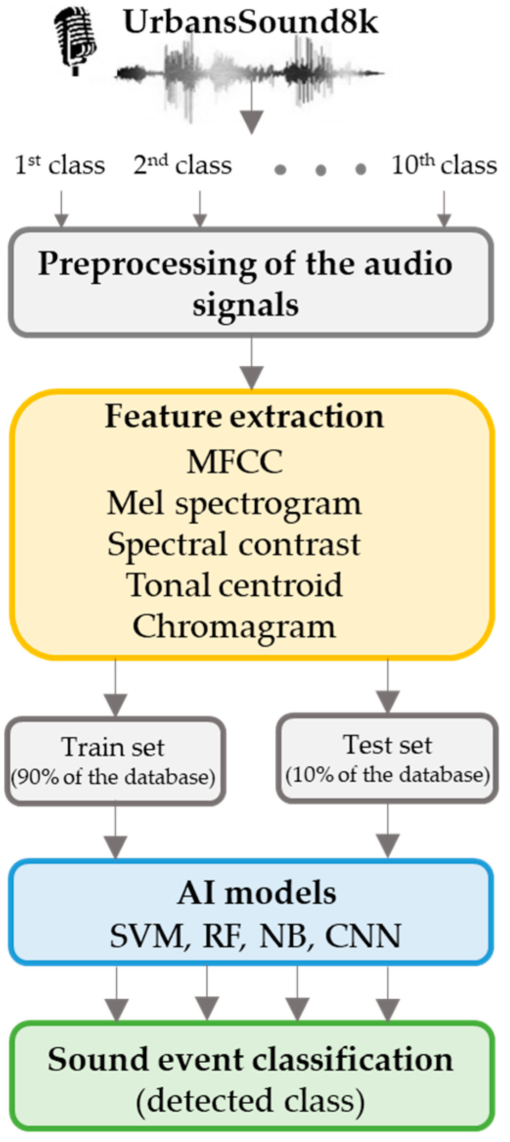
Figure 1. Architecture of the AED/C system.
Urbansci 09 00517 g001
Figure 2. Analysis of audio files from the UrbanSound8K dataset in terms of class distribution, sample rate and bit depth.
Urbansci 09 00517 g002
Figure 3. Feature extraction steps for the used audio parameters [58].
Urbansci 09 00517 g003
Figure 4. Confusion matrix of the classification while using the support vector machines (left) and Random Forest algorithm (right).
Urbansci 09 00517 g004
Figure 5. Architecture of the CNN.
Urbansci 09 00517 g005
Figure 6. Accuracy curve (left) and loss curve (right).
Urbansci 09 00517 g006
Figure 7. Confusion matrix while using CNN with MFCC (left) and the accuracy for each class (right).
Urbansci 09 00517 g007
Figure 8. Logical flow of two-step validation of the AED/C system.
Urbansci 09 00517 g008
Figure 9. Validation accuracy of the AED/C system.
Urbansci 09 00517 g009
Figure 10. Logical flow of one wireless sensor unit.
Urbansci 09 00517 g010
Figure 11. Wireless sensor unit with implemented AED/C system (WSU consisting of main board, USB microphone and external battery with additional box and cables).
Urbansci 09 00517 g011
Table 1. Performance of 48 models of AED/C using five different feature extraction techniques and three ML algorithms (Mean Accuracy ± Standard Deviation).
Random ForestSupport Vector MachinesNaive Bayes
MFCC55.07% ± 1.36%51.05% ± 1.42%47.19% ± 1.51%
MFCC + SC63.56% ± 1.28%58.78% ± 1.34%50.53% ± 1.47%
MFCC + TC57.22% ± 1.31%50.29% ± 1.39%45.04% ± 1.45%
MFCC + Ch60.08% ± 1.25%53.17% ± 1.37%47.72% ± 1.49%
MFCC + MS42.16% ± 1.41%49.91% ± 1.38%22.33% ± 1.62%
MFCC + SC + TC65.47% ± 1.22%58.66% ± 1.32%47.91% ± 1.44%
MFCC + SC + Ch66.31% ± 1.29%59.38% ± 1.33%50.78% ± 1.50%
MFCC + SC + MS58.12% ± 1.42%55.45% ± 1.35%26.33% ± 1.58%
MFCC + TC+ Ch61.31% ± 1.26%52.78% ± 1.34%48.92% ± 1.50%
MFCC + TC + MS62.22% ± 1.30%52.92% ± 1.38%48.02% ± 1.48%
MFCC + Ch +MS57.58% ± 1.33%52.21% ± 1.36%26.16% ± 1.56%
MFCC + SC + TC + Ch65.88% ± 1.27%58.42% ± 1.35%48.98% ± 1.46%
MFCC + SC + TC + MS60.45% ± 1.31%55.13% ± 1.34%29.92% ± 1.54%
MFCC + SC + Ch + MS61.41% ± 1.28%57.59% ± 1.33%26.28% ± 1.57%
MFCC + TC + Ch + MS58.13% ± 1.30%56.72% ± 1.36%26.22% ± 1.55%
All 5 parameters62.60% ± 1.29%55.67% ± 1.36%26.40% ± 1.59%
Table 2. Architecture of the CNN (types of layer, output shape and number of parameters).
Type of LayerOutput ShapeParameters
Convolution2D
(16 filters, 2 × 2 kernel size, ReLU activation unit)
(None, 39, 173, 16)80
MaxPooling(None, 19, 86, 16)0
Spatial Dropout (0, 2)(None, 19, 86, 16)0
Convolution2D
(32 filters, 2 × 2 kernel size, ReLU activation unit)
(None, 18, 85, 32)2080
MaxPooling(None, 9,4 2, 32)0
Spatial Dropout (0, 2)(None, 9, 42, 32)0
Convolution2D
(64 filters, 2 × 2 kernel size, ReLU activation unit)
(None, 8, 41, 64)8256
MaxPooling(None, 4, 20, 64)0
Spatial Dropout (0, 2)(None, 4, 20, 64)0
Convolution2D
(128 filters, 2 × 2 kernel size, ReLU activation unit)
(None, 3, 19, 128)32896
MaxPooling(None, 1, 9, 128)0
Spatial Dropout (0, 2)(None, 1, 9, 128)0
GlobalAveragePooling2D(None, 128)0
Flatten(None, 128)0
Dense 10 units (SOFTMAX output)(None, 10)1290
TOTAL NUMBER OF TRAINING PARAMETERS 44,602
Disclaimer/Publisher’s Note: The statements, opinions and data contained in all publications are solely those of the individual author(s) and contributor(s) and not of MDPI and/or the editor(s). MDPI and/or the editor(s) disclaim responsibility for any injury to people or property resulting from any ideas, methods, instructions or products referred to in the content.