Article

From Land Use Change to Ecosystem Service Sustainability: Multi-Scenario Projections for Urban Agglomerations in Arid Northwest China

by
Yusuyunjiang Mamitimin
1,2,*,
Ailijiang Nuerla
3,
Zaimire Abudushalamu
3 and
Meiling Huang
4
1
College of Geography and Remote Sensing Sciences, Xinjiang University, Urumqi 830017, China
2
Key Laboratory of Smart City and Environment Modeling of Higher Education Institute, Urumqi 830017, China
3
College of Ecology and Environment, Xinjiang University, Urumqi 830017, China
4
Academy of Education and Science, Xinjiang Uygur Autonomous Region, Urumqi 830017, China
*
Author to whom correspondence should be addressed.
Urban Sci. 2025, 9(10), 433; https://doi.org/10.3390/urbansci9100433
Submission received: 11 August 2025 / Revised: 26 September 2025 / Accepted: 14 October 2025 / Published: 21 October 2025

Abstract

Ecosystem services play a crucial role in sustaining human life, providing numerous benefits that are indispensable for our well-being. However, these vital functions are increasingly compromised by land use changes that have been instigated by human activities. This study aims to evaluate the spatiotemporal variability of ecosystem service value (ESV) within the urban agglomeration located on the northern slope of the Tianshan Mountains over a historical period stretching from 1990 to 2020, utilizing land use data to conduct a thorough analysis. Subsequently, the Future Land Use Simulation (FLUS) model was employed to forecast ESV in 2030 under three developmental pathways: Ecological Protection Scenario (EPS), Cultivated Land Protection Scenario (CLPS), and Natural Development Scenario (NDS). The evaluation incorporated six primary land classes: cultivated land, forest land, grassland, water bodies, construction land, and unused land. The FLUS model was validated with strong accuracy (overall accuracy = 0.97, Kappa = 0.94). ESV was estimated using the value coefficient method based on equivalent factors, adjusted with a local economic coefficient for crop production. All values are expressed in constant 2020 CNY without further price normalization. Our results show that between 1990 and 2020, cultivated land expanded by 27.18% (17,721 to 22,538 km2) and construction land increased by 75.91% (1926 to 3388 km2), while grassland decreased from 63,502 to 59,027 km2 and unused land declined from 106,292 to 104,690 km2. Minor changes occurred in forest land and water bodies. Total ESV decreased from 679.06 × 10⁸ CNY in 1990 to 657.67 × 10⁸ CNY in 2020, a decline of 3.15%. Regulating, supporting, and cultural services all decreased, while provisioning services increased. Spatially, vegetated areas functioned as ESV hot spots, whereas construction-degraded areas were identified as cold spots. Scenario projections for 2030 show that under the CLPS and NDS, ESV would further decline by 11.49 × 10⁸ CNY (−1.75%) and 10.18 × 10⁸ CNY (−1.55%), respectively. In contrast, the EPS is projected to increase ESV by 4.53 × 10⁸ CNY (+0.69%), reaching 662.20 × 10⁸ CNY.

1. Introduction

The swift growth of urban areas driven by worldwide urbanization has driven significant land-use changes, with natural landscapes—such as agricultural land, forests, and wetlands—increasingly being converted into urban construction areas [1,2]. Beyond reshaping the physical morphology of cities, this transformation impairs ecosystem functionality, thereby threatening the delivery of vital ecosystem services. These essential services span multiple categories: provisioning (water, food), regulating (water purification, climate regulation), cultural (aesthetic value, recreation), and supporting (biodiversity maintenance, soil formation) [3,4,5]. Unsustainable land-use practices can degrade these ecosystem services, ultimately undermining human well-being [6]. Given the dual challenges of environmental degradation and socio-economic development pressures, reconciling economic growth with ecological preservation has become a global priority. Research on the impacts of land-use change on ecosystem services is thus essential for guiding sustainable land management policies and achieving long-term development goals.
Ecosystem Service Value (ESV) refers to the economic value quantification of various benefits that humans obtain directly or indirectly from ecosystems [7,8,9]. It aims to present the services provided by natural capital for human well-being, which are often overlooked or underestimated by traditional markets, in monetary or other comparable numerical forms, so that they can be included in decision-making considerations (such as policy formulation, land use planning, cost–benefit analysis, etc.) [10]. Researchers typically group the methodologies for ecosystem service valuation into three broad categories: energy-based valuation, material flow-based valuation, and unit area-based valuation [11]. Among the prevalent methodologies for ESV, Costanza et al.’s [7] unit area value transfer approach has achieved extensive global adoption, primarily due to two pivotal strengths: First, the monetary quantification establishes a standardized metric that enables cross-ecosystem comparisons of homogeneous service functions (e.g., carbon sequestration across biomes) and intra-ecosystem evaluations of heterogeneous services (e.g., provisioning versus cultural services), significantly enhancing public accessibility to complex ecological-economic relationships. Second, this framework increases policymakers’ awareness of natural capital dependencies, thereby facilitating the evidence-based design of ecological compensation mechanisms, such as payment for watershed services or biodiversity offsets [12,13]. In 2015, Xie et al. [14] quantified the ESV across China for 2010, through the application of an ecosystem value equivalence factor method, which synthesized the foundational model of Costanza et al. [7] with principles from the expanded labor theory of value.
Land use and land cover (LULC) change modeling technology serves as an efficient tool for elucidating spatiotemporal trends, holding substantial significance for policymakers [15,16]. It not only aids in the implementation of necessary measures but also effectively fosters the sustainable protection of land resources [17]. The application of accurate models enables researchers to gain enhanced insights into the dynamics and drivers of land use change, facilitating the projection of future land use scenarios aligned with sustainable development goals. This, in turn, provides robust support for scientific management and sustainable development of land resources [18]. According to the classification of simulation methods, models can be divided into various types, including empirical statistical models, cellular automata models, economic models, and hybrid models [19,20,21,22]. Among these, the empirical statistical model and cellular automata model adopt a pattern-oriented modeling approach, while economic models and hybrid models focus on process-oriented in-depth exploration. Hybrid models, which integrate the strengths of other models to accurately simulate land use patterns in both quantitative and spatial dimensions, have emerged as the most widely applied models in contemporary land use simulation research [23,24]. These models can amalgamate various conceptual frameworks, theories, and observations, enabling modelers to select suitable simulation procedures based on practical requirements. Currently, commonly used hybrid models encompass various models and software packages applicable to future land-use simulation under different scenarios, such as the Conversion of Land Use and its Effects at Small regional extent (CLUE-S) model [25,26,27], the Patch-generating Land Use Simulation (PLUS) model [28,29,30], the Future Land Use Simulation (FLUS) model [31,32,33], and the Land Change Modeler (LCM) [34]. Notably, the applicability of the FLUS model in urban land-use simulation stems primarily from its operational simplicity and bottom-up approach.
The urban agglomeration on the northern slope of the Tianshan Mountains in Xinjiang is recognized as the largest and most developed urban cluster in China’s arid northwest. Contributing over 65% of the region’s total economic output while occupying less than 10% of Xinjiang’s land area, this zone achieved an urbanization rate of 82.8% by 2018, serving as the primary engine for industrialization, modern agriculture, and technological innovation in Xinjiang. However, as a typical mountain–oasis–desert composite ecosystem, the area exhibits extreme ecological fragility; with an average annual precipitation of merely 215 mm, it belongs to a characteristically extreme arid continental climate zone. Against the backdrop of rapid new urbanization, the continuous expansion of construction land has led to significant issues such as the compression of ecological space and the non-grain conversion of cultivated land, posing severe challenges to the region’s ecosystem service functions. Although prior research in the UANSTM region has preliminarily explored the relationship between LULC and ESV, several critical gaps remain unaddressed. Existing studies often rely on low-resolution data and short-term analyses, lack spatially explicit validation of predictive models, overlook trade-offs and synergies in specific scenarios, and fail to quantify uncertainties in ESV assessments. Addressing these limitations, this research first examines the spatiotemporal patterns of land use change in the region (1990–2020) and their effects on ESV, employing the equivalent factor method. Following this, the study leverages the FLUS model to simulate potential land use configurations for 2030 under various scenarios and to evaluate the corresponding trends in ESV evolution (Figure 1). The study advances existing knowledge in three key areas: (i) Utilizing long-term (1990–2020) high-resolution spatial data to enhance the accuracy of historical trend analysis; (ii) Designing multiple future scenarios (natural development, ecological conservation, farmland protection) to quantify policy-sensitive trade-offs—for example, we anticipate that the ecological conservation scenario will significantly enhance regulating and supporting services, although provisioning services may decline; (iii) Rigorously validating FLUS model predictions using spatially explicit metrics (overall accuracy and Kappa coefficient). By integrating these methodologies, this study provides an innovative, robust, and spatially explicit assessment of past and future dynamics of ecosystem service value across the UANSTM region. These research outcomes provide a scientific basis for spatial planning and the preservation of ecological security in arid regions undergoing urbanization.

2. Materials and Methods

2.1. Study Region

The urban agglomeration on the northern slope of the Tianshan Mountain (UANSTM) is situated in the heart of the Asia–Europe continent (83°24′~91°54′ E, 41°11′~46°18′ N), exemplifying a typical ‘mountain-basin system’ in the arid northwestern region of China (Figure 2) [35]. The study area has an average elevation of 1000 m and encompasses a total area of 215,400 km2. The climate is characterized as a temperate arid continental type, featuring a mean annual temperature of 7.4 °C. Total annual precipitation is 215 mm, which is markedly outweighed by an evaporation rate of 1825 mm. Notably, precipitation patterns are highly seasonal, with 70% occurring during the June–September period [36]. The dryness index exceeds 8.5, indicating significant aridity. The unique geographic configuration has resulted in pronounced spatial differentiation of water and heat resources, with precipitation decreasing from south to north (220 mm to 100 mm). The regional ecosystem is notably fragile, as evidenced by low vegetation cover, a high proportion of salinized soil, and a desertification expansion rate of 1.5% per annum [37]. Socio-economically, the urban agglomeration comprises four prefecture-level cities, including Urumqi and Changji, as well as seven county-level units, with a total population of 5,917,100 as of the end of 2018 and an urbanization rate of 82.8%. As the core driver of industrialization, modern agriculture, and technological innovation in Xinjiang, less than 10% of the land area is responsible for generating over 65% of the region’s GDP.

2.2. Data Source and Processing

This research integrates heterogeneous geospatial datasets from diverse sources, structured into four principal categories: (1) Terrain and land use: high-resolution land use data (30 m), and Digital Elevation Model raster layers, supplemented by derived topographic parameters (slope) generated using spatial analysis tools. The primary dataset for this analysis comprised land-use maps, which were developed based on visual interpretation of LANDSAT images. The evaluation of interpretation accuracy for all specified time points revealed consistently high results, with accuracy levels exceeding 90%. This demonstrates a significant degree of precision and reliability in the classifications across the entire study period. (2) Bioclimatic variables: precipitation composites, temperature grids, and Normalized Difference Vegetation Index (NDVI) surfaces at a spatial resolution of 1 km. (3) Infrastructure networks: vector-based transportation infrastructure (road hierarchy) and patterns of human settlement distribution. (4) Socioeconomic metrics: spatialized socioeconomic indicators, including Gross Domestic Product (GDP), population density, and nighttime light (NTL) intensity layers (Table 1). All raster datasets were transformed to the Krasovsky_1940_Albers coordinate system and resampled using nearest neighbors method to ensure a consistent resolution of 1 km. Before training the artificial neural network, categorical variables, including land use and land cover types, were subjected to one-hot encoding, while continuous variables were standardized using Z-scores.

2.3. FLUS Model

As an advanced tool within the Cellular Automata (CA) framework, the FLUS model improves the reliability of land use simulations by boosting their spatial precision and realistically representing the underlying processes. This enhancement is achieved through the integration of the Artificial Neural Network (ANN) algorithm, dynamic inertia coefficient regulation, and a probabilistic roulette wheel competition mechanism [38]. The technical architecture of the model comprises two core modules: the suitability probability calculation module, which is based on a three-layer feed-forward neural network. This module is designed to dynamically capture and represent the complex interdependencies governing land use change and its multiple drivers through a hierarchical structure that includes an input layer (spatial driving factors), an implicit layer (nonlinear feature extraction), and an output layer (transition probability generation). The researcher constructs a training set by randomly sampling historical land use data and geographic environmental variables, optimizes the network parameters using the error backpropagation algorithm, and ultimately outputs the land use transition probability for each metacellular cell, mathematically represented as:
P p , k , t = j w j , k s i g m o i d n e t j n e t j p , t = j w j , k × 1 1 + e n e t j p , t
where P p , k , t is the suitability probability of the k th land type at grid p and time t ; w j , k is the adaptive weight of the implicit layer and the output layer; s i g m o i d is the excitation function from the implicit layer to the output layer; and n e t j p , t is the received signal of the j th implicit layer grid p at time t .

2.4. Selection of the Driving Factors

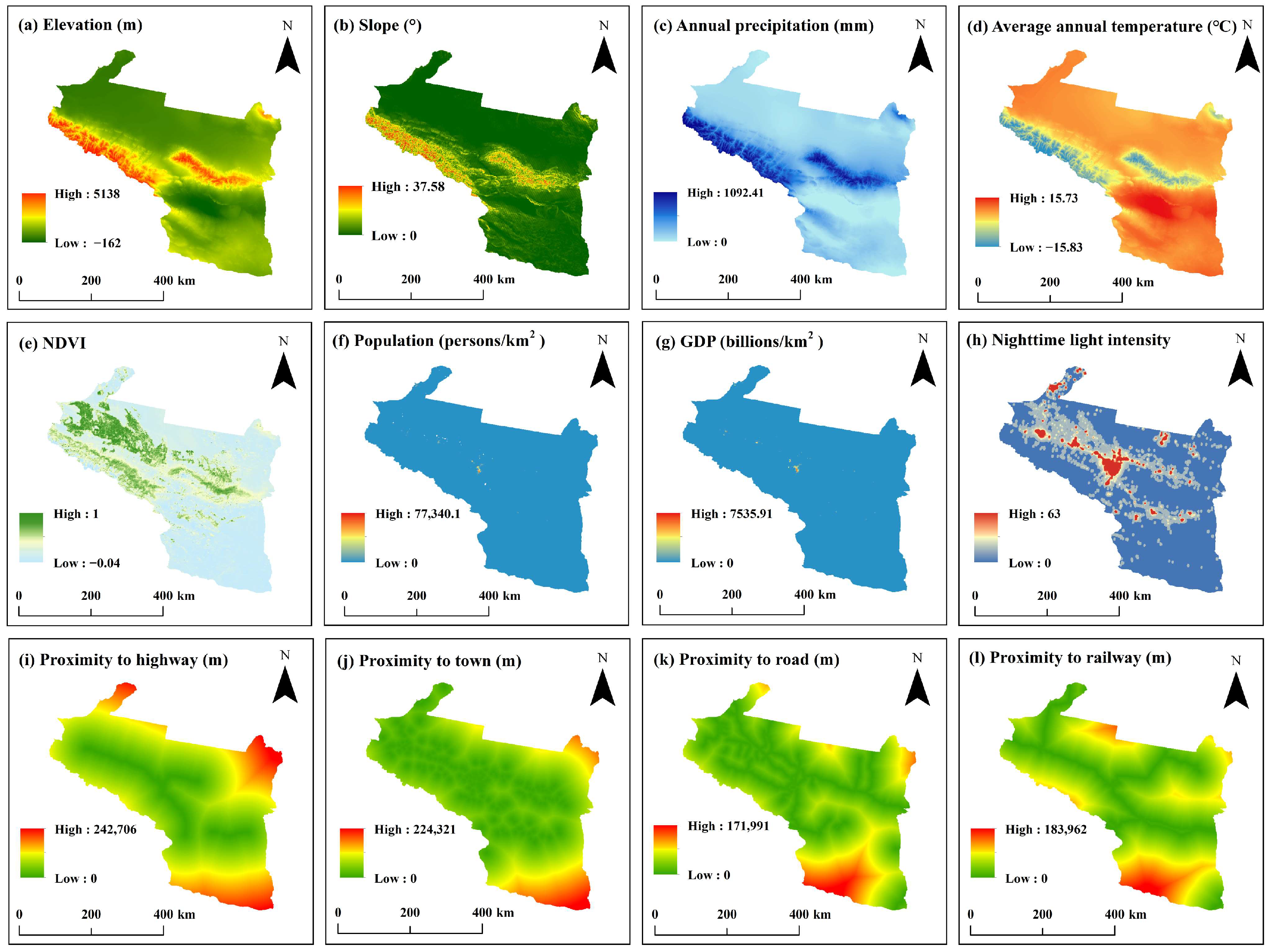
Land use dynamics demonstrate spatiotemporal nonlinearity governed by multi-scale interactions between natural and anthropogenic drivers. Through systematic analysis of the UANSTM’s unique geographical context, we identified 12 critical driving factors categorized into two domains (Figure 3): (1) biophysical determinants including elevation (30 m DEM), slope (derived through ArcGIS 10.8 Surface Analysis), bioclimatic variables (precipitation/temperature), and vegetation dynamics (MODIS NDVI composites); (2) socioeconomic influences comprising demographic-economic indicators (population density, GDP per km2 and nightime light intensity) and accessibility metrics calculated via Euclidean distance analysis to key infrastructure and settlements (urban/rural centroids). To assess collinearity within the driving factors, a Ordinary Least Squares regeression model was constructed with elevation as the dependent variable, predicted by the other 11 drivers. The analysis revealed a higher level of collinearity for the annual precipitation and mean annual temperature relative to elevation. Nevertheless, their Variance Inflation Factor (VIF) scores remained below the significant threshold, and no driving factor exhibited severe collinearity (VIF > 10) with the independent variable, elevation.

2.5. Scenario Development

Guided by relevant research and considering the current development status and future socio-economic plans for the UANSTM, three scenarios are defined as follows: The Natural Development Scenario (NDS) extrapolates future land-use patterns based on the observed change rates between 1990 and 2020, reflecting natural trends of each land type and their mutual transfer degrees without policy or planning restrictions. Regional food security and the supply of key agricultural products are the primary targets of the Cultivated Land Protection Scenario (CLPS), which seeks to achieve them through the conservation of arable land resources. It modifies the transfer cost matrix established in the NDS to restrict the conversion of arable land to other types. The Ecological Protection Scenario (EPS) seeks to maintain the ecological integrity of fragile arid-area systems by increasing the protection of forests, grasslands, and water bodies. This scenario adheres to the guidelines of the NDS, strictly limiting the conversion of ecological land to other types and curbing the expansion of construction land to maximize regional ecological benefits. The conversion mechanism of all three scenarios while simulating the future LULC with the FLUS model is reflected through the transition matrix. As shown in Table 2, the number 1 in the matrix represents that the transfer is allowed, and the number 0 represents that the transfer is restricted.

2.6. Validation of FLUS Model

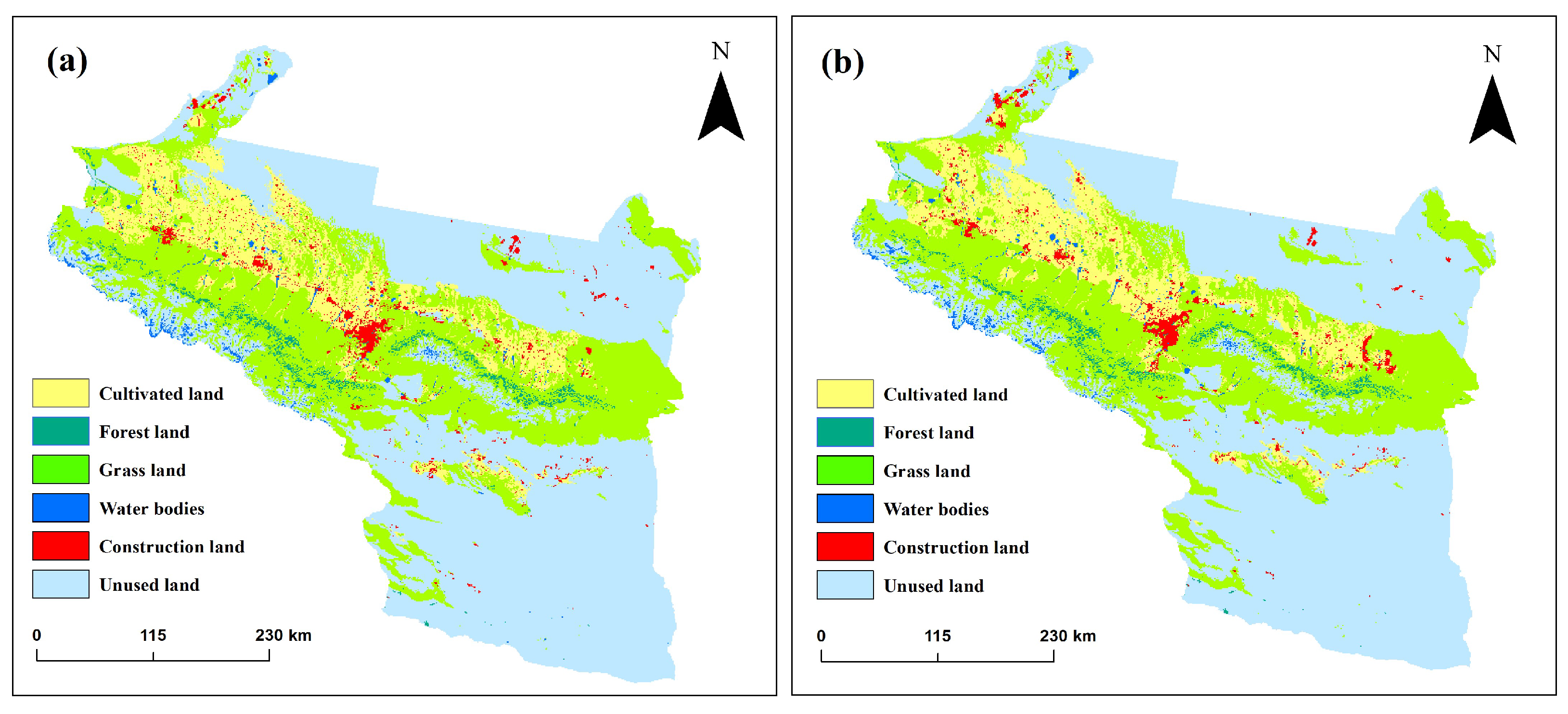
A simulation of the 2020 land use pattern was performed using 2000 and 2010 data as inputs. The outcome was then benchmarked against the actual 2020 map to validate the FLUS model’s accuracy for future projections in the UANSTM. Figure 4 serves to validate the simulation model by contrasting the projected land use distribution against the empirical data (2020) from the study area. The comparison revealed a high consistency between simulated and actual land use patterns, as reflected by the strong validation metrics (Kappa = 0.94, OA = 0.97; Table 3). The high overall performance was primarily driven by the forest and unused land classes, which achieved the highest accuracy (99.5%). In contrast, the construction land class had the lowest accuracy (58.5%), but its limited influence on the overall metrics due to a smaller sample size. These results confirm the FLUS model’s capability to accurately project future land use in the region, while also identifying construction land as a key priority for future model optimization.

2.7. Assessment of ESV

This study employed a parameter borrowing methodology for ESV assessment, integrating three established research frameworks. Building upon Costanza et al.’s foundational valuation principles [7], we specifically adopted the Chinese terrestrial ecosystem equivalent factor matrix developed by Xie et al.’s research team [14]. The comprehensive calculation framework for unit area ESV in the study region is expressed as follows:
E a = 1 7 i = 1 n m i p i q i M
where E a refers to the ESV per unit area (CNY/km2); i refers to the major crop types in the region; m i refers to the planting area of major crops; p i refers to the average market value of major crops (CNY/ton); q i is the yield per unit area of major crops (ton/km2); M refers to the total acreage of crop land.
The following formula is used to calculate the ESV for each type of land use as well as the overall ESV:
V C i , j = e i , j × E a
E S V i = j = 1 m A i × V C i , j
E S V j = i = 1 n A i × V C i , j
E S V = i = 1 n j = 1 m V C i , j × A i
where e i , j refers to the equivalent coefficient of each ES features for each land use type; V C i , j refers to the ESV for each ES feature of land use i in per unit area; A i refers to the acreage of land use i in the region; E S V i refers to the total ESV of land use i in the region; E S V j refers to the total ESV of ES feature j in the region; E S V refers to the total ESV of the region.

2.8. Spatial Autocorrelation Analysis

Spatial autocorrelation analysis captures spatial distribution patterns and quantifies the spatial dependence of geographic elements by incorporating global and local dimensions [39,40]. Global spatial autocorrelation analysis is a crucial method for examining regional spatial distribution patterns, primarily aimed at revealing the overall distribution characteristics of spatial elements within a study area. Due to its widespread application, Moran’s I is often the statistic of choice for assessing global spatial autocorrelation. It effectively captures the clustering or dispersion trends of regional spatial distributions by quantifying the degree of correlation among spatial elements. The Moran’s I statistic is computed according to the following formula:
I = n W 0 × i = 1 n j = 1 n w i j x i x ¯ x j x ¯ i = 1 n x i x ¯ 2
where I refers the Moran index, while n represents the total count of spatial elements. W 0 represents the total sum of spatial weights, w i j denotes the spatial weight between elements i and j , and x i and x j are the attribute values of the i and j spatial elements, respectively. The term x ¯ denotes the average of all spatial attribute values. The index I may assume values that fall within the interval of [−1, 1]. If I is greater than 0, this suggests a positive correlation among the spatial components; if I is less than 0, it implies a negative correlation; and if I equals 0, this indicates that there is no correlation between the spatial components.
Cold hotspot analysis is a method of local spatial autocorrelation that employs distance weights to identify clustering characteristics and their local correlation patterns within spatial data. The core functionality of this method is to discriminate between high-value and low-value clusters, achieved by analyzing the correlation between each spatial unit and its surrounding units. The calculation formula is as follows:
G i * = j = 1 n w i , j x j j = 1 n w i , j × S S i
where G i * represents the statistic value of element i , w i , j denotes the spatial weight between element i and j , and x j signifies the attribute value of the j spatial element. Furthermore, S is the cumulative sum of the attribute values of all elements, while S i refers to the cumulative sum of the attribute values of element i .

3. Results

3.1. LULC Change Analysis and Simulation Under Multiple Scenarios

The spatiotemporal dynamics of LULC in the UANSTM from 1990 to 2020 are presented in Figure 5 and Table 4. It can be observed that marked changes in land use area were recorded over this time frame, with unused land and grassland continuing to dominate the overall landscape. Spatially, over half of the area comprised unused land, predominantly in the north and south, and grassland, covering more than 30%, was mainly concentrated in the central region. Quantitatively, cultivated land witnessed an expansion of 27.18%, growing from 17,721 km2 to 22,538 km2, while construction land increased from 1926 km2 to 3388 km2, showing a 75.91% growth over the study period. Conversely, grassland area decreased from 63,502 km2 in 1990 to 59,027 km2 in 2020, while unused land area decreased from 106,292 km2 in 1990 to 104,690 km2 in 2020. In contrast, forest land and water bodies experienced relatively minor changes. Over the three-decade period from 1990 to 2020, forest cover experienced a reduction from 2900 km2 to 2596 km2, while water bodies expanded from 1693 km2 to 1741 km2, respectively.
Using the FLUS model, this study simulated future land use patterns across multiple scenarios for the year 2030, thereby exploring projected changes in land use (Figure 6 and Table 5). The projection results indicate that, under the NDS, both construction land and cultivated land are set to expand substantially, with increases of 1103 km2 and 1043 km2, respectively, relative to the 2020 baseline. This expansion coincides with a considerable reduction in unused land and grassland, which are projected to decline by 303 km2 and 1802 km2, respectively. The changes in water bodies and forest land are anticipated to be minimal. Under the CLPS, the primary changes in 2030 will be concentrated in construction land, cultivated land, grassland, and unused land. Compared to 2020, construction land and cultivated land are expected to increase by 1036 km2 and 1045 km2, respectively, with corresponding losses of 1802 km2 from grassland and 303 km2 from unused land. Substantial alterations are not anticipated for water bodies and forest land. A lower expansion rate for construction land is anticipated under the CLPS than under the NDS. Moreover, the CLPS is characterized by an increase in both cultivated land and water body areas. Restrictions on converting cultivated land to other uses primarily limit the potential for construction land development. The EPS projects a notable expansion of construction land and forest land by 365 km2 and 259 km2, respectively, by 2020. In contrast, cultivated land and unused land are forecast to contract by 452 km2 and 303 km2. Meanwhile, increases of 80 km2 in grassland and 50 km2 in water bodies are also anticipated. Simulation results reveal that the EPS effectively curtailed the considerable expansion of construction land while simultaneously achieving superior conservation of grassland and forest land compared to other scenarios.

3.2. Spatial-Temporal Changes in ESV

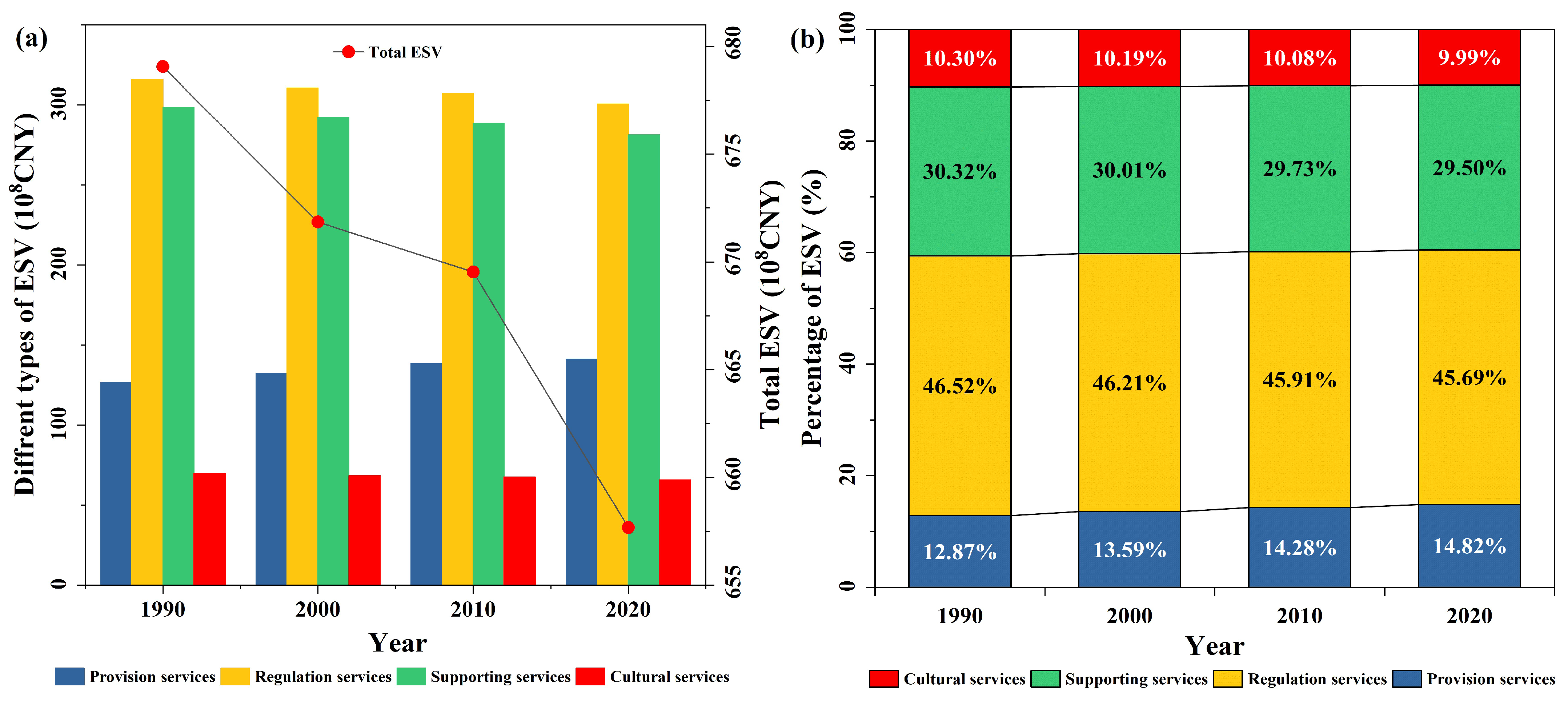
The total ESV of the UANSTM declined from 679.06 × 10⁸ CNY in 1990 to 657.67 × 10⁸ CNY in 2020, indicating a reduction of 3.15% (Figure 7 and Figure 8). Specifically, between 1990 and 2000, the total ESV experienced a sharp decline from 679.06 × 10⁸ CNY in 1990 to 671.84 × 10⁸ CNY in 2000, representing a decrease rate of 1.06%. Furthermore, from 2000 to 2010, there was a slower decline from 671.84 × 10⁸ CNY to 669.53 × 10⁸ CNY, with a decrease rate of 0.34%. In the period from 2010 to 2020, the decrease accelerated from 669.53 × 10⁸ CNY to 657.67 × 10⁸ CNY, resulting in a decrease rate of 1.77%. In the UANSTM, the changes in each type of ESV varied from 1990 to 2020. The values of regulating, supporting, and cultural services all exhibited a decreasing trend, while only provisioning services demonstrated an increasing trend. Regulating services represented the highest value, accounting for more than 45% of the total ecosystem service value, followed by supporting services representing more than 29%, provisioning services respresenting more than 12%, and cultural services at 10%.

3.3. Spatial Aggregation of ESV

The spatial distribution of ESV in the UANSTM was evaluated for clustering patterns using global spatial autocorrelation analysis. The methodological framework involved calculating Moran’s I index, followed by significance testing using permutation-based p-values (Table 6 and Figure 9). Regarding the calculation of the Moran’s I index, the spatial weight matrix was constructed using an inverse-distance method based on Euclidean distance. The analysis was conducted on a 1 km × 1 km grid. Edge effects were mitigated by ensuring a sufficient spatial extent to minimize boundary distortion. The analysis revealed consistently positive Moran’s I indices across four decadal intervals: 0.691 (1990), 0.697 (2000), 0.700 (2010), and 0.693 (2020), all statistically significant at the 99% confidence level (p < 0.01). Notably, the peak Moran’s I value of 0.700 observed in 2010 suggests optimal spatial clustering of ESVs during this period, indicating minimized spatial heterogeneity within the study area. Although subsequent measurements showed slight decreases (0.693 in 2020), the indices remained consistently elevated (range: 0.691–0.700), demonstrating remarkable temporal stability in ESV spatial distribution patterns. A noteworthy temporal pattern emerged from the longitudinal analysis: a sustained positive trend in Moran’s I values was observed over the 30-year study period, with a 0.29% increase from 1990 to 2020. This upward trajectory implies a progressive intensification of spatial aggregation and strengthened inter-correlations among ESV distribution patterns. Methodological precision was ensured through robust statistical validation, with all z-scores exceeding 2.58, confirming non-random spatial patterns. Collectively, these findings suggest that the study area maintains persistent spatial memory in ESV distribution, characterized by stable high-value clustering cores and self-reinforcing spatial correlation mechanisms.

3.4. Spatial Cold and Hot Spot Patterns of ESV

The spatial distribution of ESV hot spots and cold spots illustrates the varying levels of service provision across assessment units. Hotspots represent areas that exceed regional averages, while cold spots indicate areas with below-average performance. Non-significant areas exhibit minimal discrepancies between supply and demand. The classification system is statistically validated through hierarchical confidence levels (99%: core, 95%: priority, 90%: moderate), with areas rated below 90% confidence categorized as non-significant. As illustrated in Figure 10 and Table 7, the ESV exhibits pronounced spatial differentiation characteristics. Strong hotspot service area clusters predominantly form a spatially continuous belt that extends from the northwestern periphery to the eastern sector within the central core of the study area. In contrast, very strong cold spot service areas are located in the southern and northern regions of the study area. From a natural geographic standpoint, the central area is distinguished by high coverage of forests and grasslands, identifying it as a key ecosystem service supply area and a hub for ESV hotspots. Conversely, cold spots—located in the northern, southern, and scattered central areas—are largely composed of unused and construction land. In terms of land use, zones with greater vegetation cover generally correspond to higher ESV. Notably, forested and grassland areas provide superior soil and water conservation functions and biodiversity compared to arable land, thereby solidifying their status as ecological service hotspots. In contrast, the cold spot service areas are adversely affected by the development of construction land, which leads to irreversible damage to surface soil and vegetation. Consequently, this degradation directly results in diminished ESV for key regulatory services, including water balance, soil stability, and the maintenance of biological diversity, forming the basis for their classification as service cold spots.

3.5. ESV Analysis Under Multi-Scenarios

Based on the patterns of land use predicted for 2030 derived from FLUS model, this study further evaluates ESV of the UANSTM under different development scenarios. The prediction results reveal significant differences in ESV across various development scenarios for 2030 (Figure 11 and Table 8). Under the NDS, the ESV reaches 646.18 × 10⁸ CNY, reflecting a decrease of 11.49 × 10⁸ CNY compared to 2020. In the CLPS, the ESV is projected to be 647.79 × 10⁸ CNY, representing a decrease of 10.18 × 10⁸ CNY compared to 2020. Under the EPS, the ESV is anticipated to reach 662.20 × 10⁸ CNY, marking an increase of 4.53 × 10⁸ CNY from 2020. Analyzing the structure of ecosystem service types, regulatory services remain the primary contributor, followed by supporting services. Specifically, under the NDS and CLPS, while the value of provisioning services is projected to increase, the values of regulatory, supporting, and cultural services are expected to decline compared to 2020. In contrast, under the EPS, the value of provisioning services is expected to decrease, while the regulatory, supporting, and cultural services are projected to increase to varying degrees. The results indicate that implementing proactive ecological and environmental protection strategies can effectively reverse the declining trend in ESV and promote positive growth in the UANSTM. This highlights the critical role of an ecology-first development approach in maintaining regional ecosystem service functions.

4. Discussion

4.1. Changes in LULC and ESV in UANSTM

This paper quantifies the spatiotemporal variability of ESV within UANSTM from 1990 to 2020 using LULC data and projects future ESV for 2030 under multiple development scenarios. A key trend identified was the concurrent expansion of construction and cultivated land, accompanied by a considerable reduction in grassland extent over the study duration. Regarding ESV changes, the total ESV for UANSTM declined from 679.06 × 10⁸ CNY in 1990 to 657.67 × 10⁸ CNY in 2020, representing a reduction of 3.15%. We observe that this overall declining pattern is consistent across three ecosystem service types—regulating, supporting, and cultural services—while provisioning services exhibit continued growth. The decrease in ESV is associated with land use pattern changes, specifically the decrease in grassland and the expansion of construction land and cultivated land. Construction land generally provides lower-value ecosystem services [41]; consequently, urbanization and city expansion driving a rapid increase in construction land area between 1990 and 2020 constitute an important reason for the decline in total ESV between 1990 and 2020. Additionally, cultivated land expansion is one of the major factors contributing to the decline in ESV within the UANSTM. These findings align with other studies conducted in the arid and semi-arid regions of northwest China [42,43,44]. Although this expansion increased provisioning services, cropland’s contribution to the total ESV was significantly lower than that of grassland, forest land, and water bodies, which possess a higher value per unit area [45]. Furthermore, the expansion of cultivated land causes increased agricultural water consumption, which results in the development of surface and groundwater resources [46]. This leads to ecological problems including soil salinization, degradation, and landscape fragmentation, ultimately contributing to the decline in Total ESV [47].

4.2. From Patterns to Practice: Conservation Implications and Policy Recommendations of ESV Cold and Hot Spots

Our analysis indicates that the continuous hotspot belt precisely coincides with piedmont oasis zones and key water source conservation areas. These regions are not only rich in vegetation but also serve as essential ecological buffers, regulating water flows from the Tianshan Mountains to the arid plains. Consequently, their designation as hotspot areas highlights their irreplaceable role in regional water security, necessitating their prioritization as protected zones within spatial planning. The cold spots in the northern and southern regions, characterized by unused and construction land, signify not only current degradation but also represent key priorities for restoration. Targeting restoration efforts towards cold spots adjacent to existing hotspots could enhance ecological connectivity and foster larger, more resilient patches of high-value ecosystem service areas. Addressing the central challenge of accommodating development needs without degrading ESV in arid regions requires a strategic priority on scientific land-use management that explicitly weighs economic objectives against ecological imperatives [48]. To overcome the unique challenges facing urban agglomerations in arid regions, we propose the following recommendations for increasing regional ESV. First of all, our simulation projections indicate that the gains in ESV derived from the EPS are predominantly concentrated in identified hotspot zones and their surrounding areas. This finding underscores the critical importance of safeguarding these regions from a future scenario perspective. Therefore, it is recommended to establish an ‘Ecological Protection Redline’ specifically along the northwestern to eastern hotspot belt to legally safeguard these zones from conversion to other land uses. In addition, differentiated spatial strategies are imperative to elevate ESV in cold spots dominated by construction land and unused land. Recommendations include intensifying construction land use and expanding green spaces within urban areas, and initiating restoration of unused land through planting drought-tolerant vegetation for combined windbreak, sand fixation, and carbon sequestration benefits. Finally, the CLPS involves a clear trade-off: ensuring food supply may undermine regulating services like water catchment if natural lands are converted. A “smart” strategy should thus focus conservation on existing productive farmland and require water-saving agroecology in developable areas to mitigate impacts.

4.3. Limitations and Future Work

The assessment of ESV is a complex, profound and systematic undertaking. While this study evaluated spatiotemporal ESV evolution and its potential changes in in the future in UANSTM from a land-use dynamics perspective, we acknowledge that uncertainties persist. First of all, this study has assessed the spatiotemporal distribution of four key ecosystem service types within the UANSTM from both historical and future perspectives. However, the four ecosystem service functions examined in this study do not address all ecosystem services, including disease control, aesthetic value, and educational value, which were excluded due to data availability constraints. In future research, it is essential to comprehensively consider and evaluate all ecosystem service functions and explore their trade-off and synergistic relationships. A second limitation lies in the equivalent factor coefficient method’s exclusion of climate change effects on ecosystem services [49], which disrupt hydrological regimes and consequently drive ESV fluctuations. Coupling climate models with FLUS and ESV assessment models could deliver more robust future landscape simulations, thereby improving ESV valuation precision.

5. Conclusions

In this study, we assessed the spatiotemporal dynamics of ecosystem service value (ESV) in the Urban Agglomeration on the Northern Slope of the Tianshan Mountains (UANSTM) from 1990 to 2020 based on land use data and projected ESV changes under three scenarios for 2030 using the Future Land Use Simulation (FLUS) model. The results reveal substantial land use changes over the past three decades: while unused land (>50%) and grassland (>30%) remained dominant, cultivated land expanded markedly by 27.18%, and construction land increased dramatically by 75.91%. These changes were accompanied by declines in grassland and unused land, whereas forest and water bodies experienced minor fluctuations. Consequently, the total ESV decreased by 3.15%, from 679.06 × 10⁸ CNY in 1990 to 657.67 × 10⁸ CNY in 2020. Among ESV categories, regulating, supporting, and cultural services all declined, while only provisioning services increased. Regulating services constituted the largest share (>45%), followed by supporting services (>29%). Spatial analysis identified a distinct northwest–east hotspot belt characterized by high vegetation cover, which delivered key ecosystem services including conservation of soil and water. In contrast, cold spots clustered in the northern and southern regions, dominated by unused and construction land, where ecosystem functions were significantly degraded. These patterns, statistically significant at confidence levels of 90%, 95%, and 99%, highlight clear spatial priorities: the hotspot belt should be prioritized for conservation, while cold spots warrant targeted restoration. Scenario projections for 2030 show divergent ESV trajectories. Under the NDS and CLPS, ESV would further decline by 11.49 × 10⁸ CNY and 10.18 × 10⁸ CNY, respectively. In contrast, the EPS would reverse this trend, increasing ESV by 4.53 × 10⁸ CNY. These results underscore that an ecology-oriented development pathway is essential for sustaining regional ecosystem services. Despite these insights, key uncertainties remain, particularly regarding the integration of climate feedbacks, water allocation constraints, and socio-economic drivers into the assessment framework. Future models incorporating these factors will enhance the robustness of ESV estimations and provide more reliable support for spatial planning in this arid and ecologically sensitive region.

Author Contributions

Conceptualization, Y.M., A.N., Z.A. and M.H.; Formal analysis, Y.M.; Funding acquisition, A.N.; Methodology, Y.M.; Software, Y.M.; Supervision, A.N.; Validation, Y.M.; Visualization, Y.M. and M.H.; Writing—original draft, Y.M. and M.H.; Writing—review & editing, Y.M., A.N. and Z.A. All authors have read and agreed to the published version of the manuscript.

Funding

This research was funded by the Tianshan Talent Training Program of Xinjiang Uygur Autonomous Region (No. 2024TSYCCX0014) and the Natural Sciences Foundation of Xinjiang Uygur Autonomous Region (Grant No.: 2024D01C19).

Data Availability Statement

All original contributions of this study are included in the article itself, and further inquiries should be addressed to the corresponding author.

Acknowledgments

We sincerely appreciate the anonymous reviewers for their insightful suggestions, which have helped enhance the quality of this work.

Conflicts of Interest

The authors state that there are no conflicts of interest.

Abbreviations

The following abbreviations are used in this manuscript:
ESVEcosystem Service Value
FLUSFuture Land Use Simulation
UANSTMUrban Agglomeration on the Northern Slope of the Tianshan Mountains
NDSNatural Development Scenario
CLPSCultivated Land Protection Scenario
EPSEcological Protection Scenario
LULCLand Use and Land Cover
CLUE-SConversion of Land Use and its Effects at Small regional extent
PLUSPatch-generating Land Use Simulation
LCMLand Change Modeler
DEMDigital Elevation Model
NDVINormalized Difference Vegetation Index
GDPGross Domestic Product
NTLNighttime Light
CACellular Automata
ANNArtificial Neural Network

References

  1. Seto, K.; Güneralp, B.; Hutyra, L. Global forecasts of urban expansion to 2030 and direct impacts on biodiversity and carbon pools. Proc. Natl. Acad. Sci. USA 2012, 109, 16083–16088. [Google Scholar] [CrossRef] [PubMed]
  2. Polydoros, A.; Cartalis, C. Assessing the impact of urban expansion to the state of thermal environment of peri-urban areas using indices. Urban Clim. 2015, 14, 166–175. [Google Scholar] [CrossRef]
  3. Xiao, R.; Lin, M.; Fei, X.; Li, Y.; Zhang, Z.; Meng, Q. Exploring the interactive coercing relationship between urbanization and ecosystem service value in the Shanghai–Hangzhou Bay Metropolitan Region. J. Clean. Prod. 2020, 253, 119803. [Google Scholar] [CrossRef]
  4. Watson, R.T.; Scientist, C.; Bank, W.; Arico, S.; Bridgewater, P.; Tschirley, J.; Valentini, R.; Almeida, F.; Barnard, P.; Invasive, G. Ecosystems and Human Well Being; Millenium Ecosystem Assessment; World Resources Institute: Washington, DC, USA, 2005. [Google Scholar]
  5. Shifaw, E.; Sha, J.; Li, X.; Bao, Z.; Zhou, Z. An insight into land-cover changes and their impacts on ecosystem services before and after the implementation of a comprehensive experimental zone plan in Pingtan island, China. Land Use Policy 2019, 82, 631–642. [Google Scholar] [CrossRef]
  6. Verburg, P.H.; Neumann, K.; Nol, L. Challenges in using land use and land cover data for global change studies. Glob. Change Biol. 2011, 17, 974–989. [Google Scholar] [CrossRef]
  7. Costanza, R.; d’Arge, R.; de Groot, R.; Farber, S.; Grasso, M.; Hannon, B.; Limburg, K.; Naeem, S.; O’Neill, R.V.; Paruelo, J.; et al. The value of the world’s ecosystem services and natural capital. Nature 1997, 387, 253–260. [Google Scholar] [CrossRef]
  8. Xie, G.; Zhang, C.; Zhen, L.; Zhang, L. Dynamic changes in the value of China’s ecosystem services. Ecosyst. Serv. 2017, 26, 146–154. [Google Scholar] [CrossRef]
  9. Liu, S.; Costanza, R.; Farber, S.; Troy, A. Valuing Ecosystem Services: Theory, Practice, and the Need for a Transdisciplinary Synthesis; Wiley/Blackwell: Hoboken, NJ, USA, 2010. [Google Scholar]
  10. Kang, Z.; Ling, H.; Gong, Y.; Yan, J.; Han, F.; Shan, Q.; Zhang, G. The precise implementation of the ecological water transfer project effectively promotes the enhancement of desert riparian ecosystem service value in the mainstream of Tarim River. Ecol. Indic. 2024, 169, 112914. [Google Scholar] [CrossRef]
  11. Jiang, W.; Wu, T.; Fu, B. The value of ecosystem services in China: A systematic review for twenty years. Ecosyst. Serv. 2021, 52, 101365. [Google Scholar] [CrossRef]
  12. Kang, N.; Hou, L.; Huang, J.; Liu, H. Ecosystem services valuation in China: A meta-analysis. Sci. Total Environ. 2022, 809, 151122. [Google Scholar] [CrossRef] [PubMed]
  13. Yang, P.; Alifujiang, Y.; Jiang, Y.; Feng, J. Study on the evaluation of ecosystem service values of typical lakes in Xinjiang. J. Nat. Conserv. 2025, 86, 126906. [Google Scholar] [CrossRef]
  14. Xie, G.D.; Zhang, C.X.; Zhang, L.M.; Chen, W.H.; Li, S.M. Improvement of the Evaluation Method for Ecosystem Service Value Based on Per Unit Area. J. Nat. Resour. 2015, 30, 1243–1254. [Google Scholar]
  15. Britz, W.; Verburg, P.H.; Leip, A. Modelling of land cover and agricultural change in Europe: Combining the CLUE and CAPRI-Spat approaches. Agric. Ecosyst. Environ. 2011, 142, 40–50. [Google Scholar] [CrossRef]
  16. Samie, A.; Deng, X.; Jia, S.; Chen, D. Scenario-Based Simulation on Dynamics of Land-Use-Land-Cover Change in Punjab Province, Pakistan. Sustainability 2017, 9, 1285. [Google Scholar] [CrossRef]
  17. Veldkamp, A.; Lambin, E.F. Predicting land-use change. Agric. Ecosyst. Environ. 2001, 85, 1–6. [Google Scholar] [CrossRef]
  18. Loukika, K.N.; Keesara, V.R.; Buri, E.S.; Sridhar, V. Future prediction of scenario based land use land cover (LU&LC) using DynaCLUE model for a river basin. Ecol. Inform. 2023, 77, 102223. [Google Scholar] [CrossRef]
  19. De Rosa, M.; Knudsen, M.T.; Hermansen, J.E. A comparison of Land Use Change models: Challenges and future developments. J. Clean. Prod. 2016, 113, 183–193. [Google Scholar] [CrossRef]
  20. Shuai, Q.; Xue, J.; Dai, L.; Huang, Y.; Jin, D.; Chen, Z.; Li, M.; Shi, Z.; Chen, S. The effects of land use change on soil organic carbon stock in China: A meta-analysis with the empirical modeling approach. Geoderma Reg. 2024, 36, e00774. [Google Scholar] [CrossRef]
  21. Liang, Z.; Liang, X.; Jiang, X.; Li, T.; Guan, Q. Balancing simulation performance and computational intensity of CA models for large-scale land-use change simulations. Environ. Model. Softw. 2025, 185, 106293. [Google Scholar] [CrossRef]
  22. Duan, X.; Haseeb, M.; Tahir, Z.; Mahmood, S.A.; Tariq, A. Analyzing and predicting land use and land cover dynamics using multispectral high-resolution imagery and hybrid CA-Markov modeling. Land Use Policy 2025, 157, 107655. [Google Scholar] [CrossRef]
  23. Li, S.-H.; Lin, W. A hybrid landscape metric-enhanced cellular automata model (LE-CA) for land use/land cover change simulation: An application to coastal wetlands. Ecol. Model. 2025, 508, 111209. [Google Scholar] [CrossRef]
  24. Molinero-Parejo, R.; Aguilera-Benavente, F.; Gómez-Delgado, M.; Shurupov, N. Combining a land parcel cellular automata (LP-CA) model with participatory approaches in the simulation of disruptive future scenarios of urban land use change. Comput. Environ. Urban Syst. 2023, 99, 101895. [Google Scholar] [CrossRef]
  25. Kiziridis, D.A.; Mastrogianni, A.; Pleniou, M.; Tsiftsis, S.; Xystrakis, F.; Tsiripidis, I. Improving the predictive performance of CLUE-S by extending demand to land transitions: The trans-CLUE-S model. Ecol. Model. 2023, 478, 110307. [Google Scholar] [CrossRef]
  26. Liao, G.; He, P.; Gao, X.; Lin, Z.; Huang, C.; Zhou, W.; Deng, O.; Xu, C.; Deng, L. Land use optimization of rural production–living–ecological space at different scales based on the BP–ANN and CLUE–S models. Ecol. Indic. 2022, 137, 108710. [Google Scholar] [CrossRef]
  27. Luo, G.; Yin, C.; Chen, X.; Xu, W.; Lu, L. Combining system dynamic model and CLUE-S model to improve land use scenario analyses at regional scale: A case study of Sangong watershed in Xinjiang, China. Ecol. Complex. 2010, 7, 198–207. [Google Scholar] [CrossRef]
  28. Liu, J.; Kong, X.; Zhu, Y.; Zhang, B. A study on land use change simulation based on PLUS model and the U-net structure: A case study of Jilin Province. Ecol. Indic. 2025, 176, 113619. [Google Scholar] [CrossRef]
  29. Gao, X.; Hu, Y.; Zhang, Z.; Jiao, Y.; Ji, W.; Qian, Y.; He, Y.; Pei, L.; Yin, Y.; Hu, Y.; et al. Analysis of the spatiotemporal evolution of cultivated land in the Chaohu Basin based on the PLUS model and multi-scenario simulation. Sustain. Futures 2025, 10, 100945. [Google Scholar] [CrossRef]
  30. Zhu, Z.; Zhao, S.; Li, Q.; Shi, Z.; Wu, Y.; Wang, L. Spatiotemporal evolution and prediction of land use change and carbon storage in ionic rare earth mining areas based on the YOLOv11–SegFormer–InVEST–PLUS integrated model. Ecol. Indic. 2025, 178, 113983. [Google Scholar] [CrossRef]
  31. Huang, M.; Mamitimin, Y.; Abulizi, A.; Yimaer, R.; Tiemuerbieke, B.; Chen, H.; Tao, T.; Ma, Y. Integrated assessment of land use and carbon storage changes in the Tulufan-Hami Basin under the background of urbanization and climate change. Int. J. Appl. Earth Obs. Geoinf. 2024, 135, 104261. [Google Scholar] [CrossRef]
  32. Mamitimin, Y.; Simayi, Z.; Mamat, A.; Maimaiti, B.; Ma, Y. FLUS Based Modeling of the Urban LULC in Arid and Semi-Arid Region of Northwest China: A Case Study of Urumqi City. Sustainability 2023, 15, 4912. [Google Scholar] [CrossRef]
  33. Liu, P.; Hu, Y.; Jia, W. Land use optimization research based on FLUS model and ecosystem services–setting Jinan City as an example. Urban Clim. 2021, 40, 100984. [Google Scholar] [CrossRef]
  34. Mumtaz, F.; Li, J.; Liu, Q.; Arshad, A.; Dong, Y.; Liu, C.; Zhao, J.; Bashir, B.; Gu, C.; Wang, X.; et al. Spatio-temporal dynamics of land use transitions associated with human activities over Eurasian Steppe: Evidence from improved residual analysis. Sci. Total Environ. 2023, 905, 166940. [Google Scholar] [CrossRef]
  35. Chen, J.; Kasimu, A.; Tang, L.; Han, F.; Jumai, M. Ecosystem service trade-offs and synergies based on the mechanical equilibrium model: A case study of the urban agglomeration on the northern slope of the Tianshan Mountains. Ecol. Indic. 2025, 177, 113795. [Google Scholar] [CrossRef]
  36. Song, X.; Chen, F.; Sun, Y.; Ma, J.; Yang, Y.; Shi, G. Effects of land utilization transformation on ecosystem services in urban agglomeration on the northern slope of the Tianshan Mountains, China. Ecol. Indic. 2024, 162, 112046. [Google Scholar] [CrossRef]
  37. Yu, T.; Abulizi, A.; Xu, Z.; Jiang, J.; Akbar, A.; Ou, B.; Xu, F. Evolution of environmental quality and its response to human disturbances of the urban agglomeration in the northern slope of the Tianshan Mountains. Ecol. Indic. 2023, 153, 110481. [Google Scholar] [CrossRef]
  38. Liu, X.; Liang, X.; Li, X.; Xu, X.; Ou, J.; Chen, Y.; Li, S.; Wang, S.; Pei, F. A future land use simulation model (FLUS) for simulating multiple land use scenarios by coupling human and natural effects. Landsc. Urban Plan. 2017, 168, 94–116. [Google Scholar] [CrossRef]
  39. Zhu, M.; Yu, X.; Chen, K.; Tan, H.; Yuan, J. Spatiotemporal characteristics and driving factors of chemical oxygen demand emissions in China’s wastewater: An analysis based on spatial autocorrelation and geodetector. Ecol. Indic. 2024, 166, 112308. [Google Scholar] [CrossRef]
  40. Lanorte, A.; Danese, M.; Lasaponara, R.; Murgante, B. Multiscale mapping of burn area and severity using multisensor satellite data and spatial autocorrelation analysis. Int. J. Appl. Earth Obs. Geoinf. 2013, 20, 42–51. [Google Scholar] [CrossRef]
  41. Cheng, X.; Chen, L.; Sun, R.; Kong, P. Land use changes and socio-economic development strongly deteriorate river ecosystem health in one of the largest basins in China. Sci. Total Environ. 2018, 616–617, 376–385. [Google Scholar] [CrossRef]
  42. Abulizi, A.; Yang, Y.; Mamat, Z.; Luo, J.; Abdulslam, D.; Xu, Z.; Zayiti, A.; Ahat, A.; Halik, W. Land-Use Change and its Effects in Charchan Oasis, Xinjiang, China. Land Degrad. Dev. 2017, 28, 106–115. [Google Scholar] [CrossRef]
  43. Muyibul, Z.; Jianxin, X.; Muhtar, P.; Qingdong, S.; Run, Z. Spatiotemporal changes of land use/cover from 1995 to 2015 in an oasis in the middle reaches of the Keriya River, southern Tarim Basin, Northwest China. Catena 2018, 171, 416–425. [Google Scholar] [CrossRef]
  44. Wang, S.; Wu, B.; Yang, P. Assessing the changes in land use and ecosystem services in an oasis agricultural region of Yanqi Basin, Northwest China. Environ. Monit. Assess. 2014, 186, 8343–8357. [Google Scholar] [CrossRef] [PubMed]
  45. Arowolo, A.O.; Deng, X.; Olatunji, O.A.; Obayelu, A.E. Assessing changes in the value of ecosystem services in response to land-use/land-cover dynamics in Nigeria. Sci. Total Environ. 2018, 636, 597–609. [Google Scholar] [CrossRef] [PubMed]
  46. Disse, M. Sustainable land and water management of River Oases along the Tarim River. In Proceedings of the International Water Resources Management Conference of ICWRS, Prague, Czech Republic, 18–20 July 2017. [Google Scholar]
  47. Zhang, Z.; Xia, F.; Yang, D.; Huo, J.; Wang, G.; Chen, H. Spatiotemporal characteristics in ecosystem service value and its interaction with human activities in Xinjiang, China. Ecol. Indic. 2020, 110, 105826. [Google Scholar] [CrossRef]
  48. Li, X.; Wu, C. Sensitivity assessment and simulation of ecosystem services in response to land use change in arid regions: Empirical evidence from Xinjiang, China. Ecol. Indic. 2025, 171, 113150. [Google Scholar] [CrossRef]
  49. Xu, C.; Jiang, W.; Huang, Q.; Wang, Y. Ecosystem services response to rural-urban transitions in coastal and island cities: A comparison between Shenzhen and Hong Kong, China. J. Clean. Prod. 2020, 260, 121033. [Google Scholar] [CrossRef]
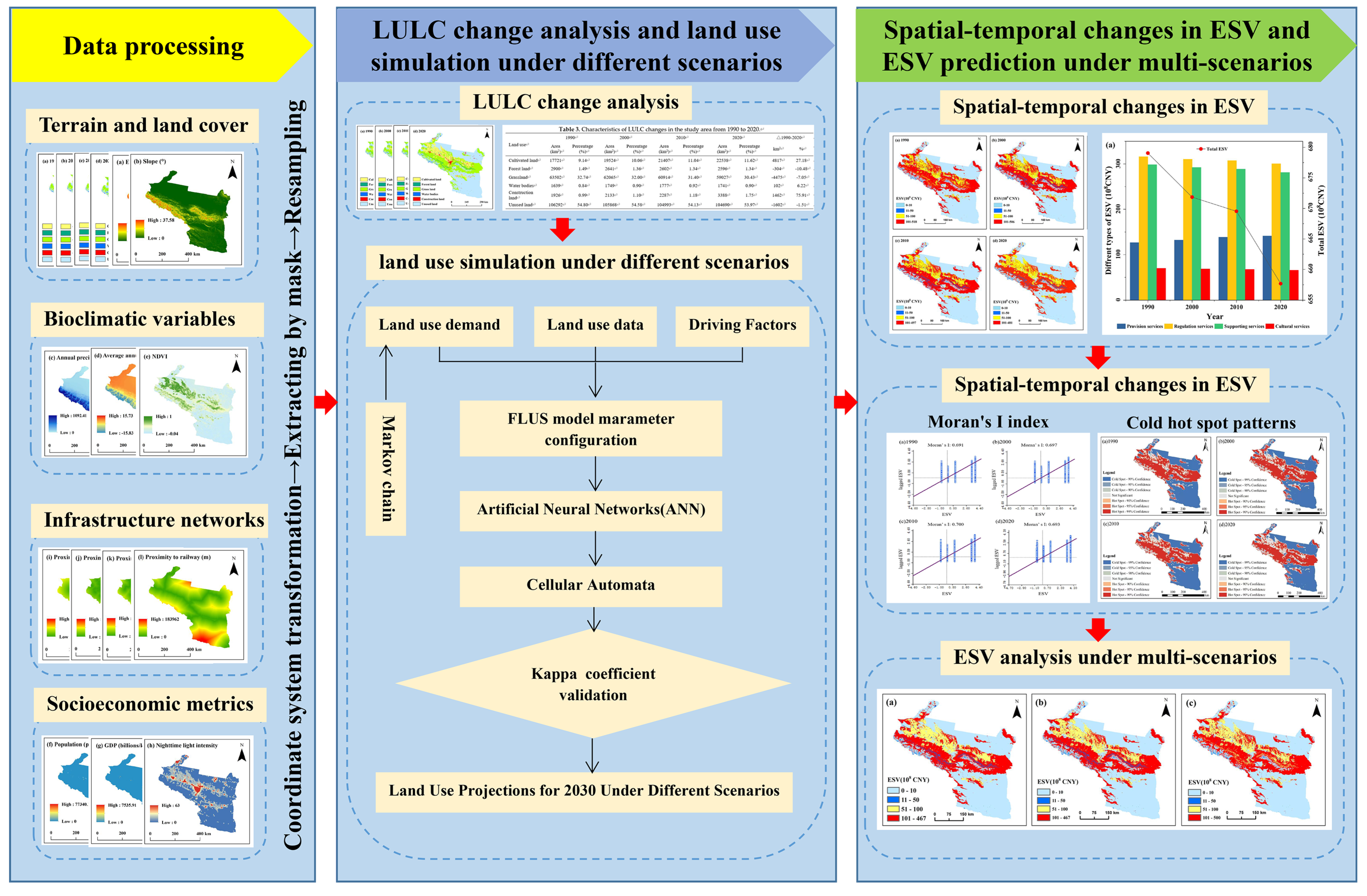
Figure 1. Research framework.
Urbansci 09 00433 g001
Figure 2. Geographical location (a) and topographic map (b) of the study area.
Urbansci 09 00433 g002
Figure 3. Driving factors affecting LULC.
Urbansci 09 00433 g003
Figure 4. LULC in 2020 ((a): actual; (b): simulated).
Urbansci 09 00433 g004
Figure 5. LULC spatial variation from 1990 to 2020 in UANSTM.
Urbansci 09 00433 g005
Figure 6. The projected LULC of UANSTM in 2030 for different scenarios ((a): NDS; (b): CLPS; (c): EPS).
Urbansci 09 00433 g006
Figure 7. Spatial dynamics of ESV (1990–2020) in UANSTM.
Urbansci 09 00433 g007
Figure 8. Change in ESV from 1990 to 2020 in UANSTM ((a): temporal dynamics of total and categorical ESV; (b): relative percentage change by ESV category).
Urbansci 09 00433 g008
Figure 9. Moran scatterplot of the ESV from 1990 to 2020 in UANSTM.
Urbansci 09 00433 g009
Figure 10. Distribution of ESV hot and cold spots from 1990 to 2020 in UANSTM.
Urbansci 09 00433 g010
Figure 11. Comparative analysis of projected ESV spatial patterns for 2030 across Scenarios ((a): NDS; (b): CLPS; (c): EPS).
Urbansci 09 00433 g011
Table 1. Summary of data sources utilized in this study.
Data CategoriesData NameData SourcesSpatial Resolution
Terrain and land useLand use dataResource and Environment Science and Data Center, Chinese Academy of Sciences (https://www.resdc.cn/)30 m
DEMGeospatial Data Cloud site, Computer Network Information Center, Chinese Academy of Sciences (https://www.gscloud.cn/)30 m
SlopeComputational generation30 m
Bioclimatic variablesAverage annual precipitationNational Centers for Environmental Information (https://www.ncei.noaa.gov/)1 km
Average annual temperature1 km
NDVIResource and Environment Science and Data Center, Chinese Academy of Sciences (https://www.resdc.cn/)1 km
Socioeconomic metricsPopulationResource and Environment Science and Data Center, Chinese Academy of Sciences (https://www.resdc.cn/)1 km
GDP1 km
NTL500 m
Crop planting area and total production dataStatistical Yearbook of Xinjiang, China-
Infrastructure networksTransportation network data and human settlement distributionNational Geographic Information Public Service Platform (https://www.tianditu.gov.cn/)-
Table 2. Land use conversion matrix.
ScenarioNDSCLPSEPS
CuFoGrWaCoUnCuFoGrWaCoUnCuFoGrWaCoUn
Cu111010100000111010
Fo111010111010010000
Gr111010111010011100
Wa000100000100000100
Co111110111110111110
Un111111111111111111
Note: Cu: Cultivated land, Fo: Forest land, Gr: Grassland, Wa: Water bodies, Co: Construction land, Un: Unused land.
Table 3. Confusion matrix.
Land UseCultivated LandForest LandGrass LandWater BodiesConstruction LandUnused Land
Cultivated land200011442725
Forest land12700000
Grass land1661560694433
Water bodies20418212
Construction land3609602013
Unused land501443410,460
Producer’s Accuracy0.900.990.960.920.571.00
User’s Accuracy0.901.000.960.950.600.99
Kappa Coefficient: 0.94, Overall Accuracy: 0.97
Table 4. Characteristics of LULC changes in the study area from 1990 to 2020.
Land Use1990200020102020△1990–2020
Area (km2)Percentage (%)Area (km2)Percentage (%)Area (km2)Percentage (%)Area (km2)Percentage (%)km2%
Cultivated land17,7219.1419,52410.0621,40711.0422,53811.62481727.18
Forest land29001.4926411.3626021.3425961.34−304−10.48
Grassland63,50232.7462,06532.0060,91431.4059,02730.43−4475−7.05
Water bodies16390.8417490.9017770.9217410.901026.22
Construction land19260.9921331.1022871.1833881.75146275.91
Unused land106,29254.80105,86854.58104,99354.13104,69053.97−1602−1.51
Table 5. Characteristics of LULC changes in 2030 for different scenarios.
Land UseArea of Land Use in 2030 (km2) △2020–2030 (km2 and %)
NDSCLPSEPSNDS%CLPS%EPS%
Cultivated land23,58123,58322,08610434.6310454.64−452−2.01
Forest land259025902855−6−0.23−6−0.232599.98
Grassland57,22557,22559,107−1802−3.05−1802−3.05800.14
Water bodies170617711792−35−2.01301.72512.93
Construction land449144243753110332.56103630.5836510.77
Unused land104,387104,387104,387−303−0.29−303−0.29−303−0.29
Table 6. Global Moran’s I of the ESV.
YearMoran’s IZ Scoresp Value
19900.6911146.21050.001
20000.69671175.49110.001
20100.7001167.63740.001
20200.69331153.32850.001
Table 7. Change in ESV hot and cold spots from 1990 to 2020 in UANSTM.
YearCold Spot-99% Confidence
(Area, km2)
%Cold Spot-95% Confidence
(Area, km2)
%Cold Spot-90% Confidence
(Area, km2)
%Hot Spot—90% Confidence
(Area, km2)
%Hot Spot—95% Confidence
(Area, km2)
%Hot Spot—99% Confidence
(Area, km2)
%
199089,73024.97338825.16181026.81256521.44581624.5465,02925.84
200089,99025.04341325.35162324.04281223.51617726.0663,50025.24
201089,81524.99329624.48158723.51314326.28613525.8862,42024.81
202089,84725.00336925.02173025.63344128.77557423.5260,68324.12
Table 8. Changes in ESV in 2020–2030 under different scenarios.
ESVESV in 2030 (108 CNY)ESV Change in 2020–2030 (108 CNY)
NDSCLPSEPSNDSCLPSEPS
PS99.1499.2696.661.681.80−0.80
RS293.81294.41303.12−6.66−6.062.65
SS189.26189.61195.86−4.78−4.431.82
CS63.9764.2066.55−1.72−1.490.86
Total646.18647.49662.20−11.49−10.184.53
Disclaimer/Publisher’s Note: The statements, opinions and data contained in all publications are solely those of the individual author(s) and contributor(s) and not of MDPI and/or the editor(s). MDPI and/or the editor(s) disclaim responsibility for any injury to people or property resulting from any ideas, methods, instructions or products referred to in the content.