Article

Non-Linear Impacts of Social and Ecological Drivers on Ecosystem Services: A Threshold Perspective

1
Land Consolidation and Rehabilitation Center, Ministry of Natural Resource, Beijing 100035, China
2
School of Resource and Environment Sciences, Wuhan University, Wuhan 430079, China
3
Department of Building and Real Estate, Research Institute of Sustainable Urban Development, The Hong Kong Polytechnic University, Hong Kong 999077, China
4
Saw Swee Hock School of Public Health, National University of Singapore, Singapore 117549, Singapore
5
School of Economics and Management, China University of Geosciences, Wuhan 430074, China
6
Laboratory of Digital Cartography and Land Information Application Engineering, Ministry of Natural Resources, Wuhan 430079, China
7
Hubei Luojia Laboratory, Wuhan University, Wuhan 430079, China
*
Author to whom correspondence should be addressed.
Urban Sci. 2025, 9(10), 390; https://doi.org/10.3390/urbansci9100390
Submission received: 26 July 2025 / Revised: 8 September 2025 / Accepted: 10 September 2025 / Published: 26 September 2025

Abstract

Exploring the impact of socio-ecological drivers on ecosystem services (ESs) is critical to ES conservation and restoration. Although a considerable amount of the literature has focused on this topic, few studies have investigated the non-linear impact thresholds of socio-ecological drivers on ESs from a global perspective. In this study, multisource geospatial data was integrated with ecological modeling to quantify six typical ESs in Wuhan, China. Dominant drivers were identified through random forests, and non-linear relationships and thresholds were analyzed by partial dependence analysis. The results revealed that elevator, distance from rivers, soil organic carbon content, aggregation index, and Shannon diversity index were the dominant drivers of most ESs. Moreover, three types of non-linear impact thresholds exist in the relationship between ESs and their socio-ecological drivers: “single threshold” effects; “monotonic impact” effects; and “complex curve” effects, including “S-shape”, “inverted U-shape” and “inverted S-shape” effects. Based on these findings, we proposed policy guidance to inform ecological protection and restoration aimed at enhancing ES provision and promoting sustainable development.

1. Introduction

Ecosystem services (ESs) represent the goods and services that humans obtain from ecosystems for their survival and development [1]. These services can be broadly categorized into four types: provision services (e.g., food production and timber supply), regulation services (e.g., air purification, water regulation, and carbon storage), supportive services (e.g., biodiversity), and cultural services (e.g., outdoor recreation and historical recognition). A global assessment report reveals that ESs are facing a general downward trend worldwide, manifested by a severe decline in wetlands, habitat degradation, biodiversity loss, etc. [2]. China is also confronting ES degradation due to over-exploitation, inappropriate use of natural resources, and a reduction in critical ecological areas, as revealed by National Survey and Assessment of Changes in Ecological Conditions (2015–2020) reports. In this context, rationally and scientifically planning, organizing, and managing ESs is crucial.
Since the concept of ESs was introduced, both theoretical understanding and practical applications have matured. Current ES research primarily focuses on the definition and classification [3], the assessment and mapping methodologies [4], the driving mechanisms [5], the interrelationships among different ESs [6], and the application of ESs in landscape planning [7]. Although significant progress has been made in ES assessment and mapping, the integration of ESs into landscape planning has progressed relatively slowly. Some scholars have made attempts, for instance, using ESs as a basis for constructing ecological security patterns [8], delineating ecological conservation redlines [9], identifying ecological conservation and restoration zones [10], and informing ecological compensation. Nevertheless, few studies have effectively applied ESs to guide the selection of specific ecological restoration measures. The core steps involve clearly identifying areas of low ES provision, determining the key factors influencing ESs, and understanding how these factors affect ESs. Therefore, exploring the intrinsic mechanisms driving ES formation and spatial patterning is a fundamental prerequisite for effective ES management and restoration.
Existing research commonly categorizes the drivers of ESs into two primary domains: natural conditions and socio-economic factors. Natural conditions—including climate, topography, and soil properties—establish the foundation for ES provision through direct biophysical constraints. Climate change, in particular, is projected to be the predominant driver of ES changes by the end of the 21st century [11]. Key socio-economic drivers include land use and land cover (LULC) change, urbanization, infrastructure development, forestry activities (plantation and reforestation), and other human interventions. These factors can directly or indirectly alter ESs [12]. As LULC change bridges socio-economic activities with ecosystem structure and function, it is widely recognized as a crucial driver of ESs [2,13]. While existing studies have examined the impacts of specific drivers, a comparative analysis of diverse drivers selected from a socio-ecological system perspective remains lacking.
Methodologically, prior research has employed diverse mathematical and statistical techniques to quantify the impacts of socio-ecological drivers on ESs. Linear regression approaches—notably ordinary least squares and correlation analysis—are frequently adopted for this purpose [14,15]. However, these methods typically focus on individual ESs while neglecting the multiple services co-produced by ecosystems. To overcome this drawback, Mouchet et al. [16] applied redundancy analysis (RDA) to simultaneously examine correlations between multiple ESs and their drivers. Nevertheless, RDA struggles with local multicollinearity among explanatory variables. Alternatively, Hu et al. [17] utilized the Geodetector model, which effectively eliminates multicollinearity but can only determine effect magnitude, not directionality. Collectively, these methods exhibit limitations in revealing complex non-linear relationships between bundled ESs and their socio-ecological drivers.
Recent studies increasingly employ machine learning methods to analyze drivers of ESs. For example, Kang et al. [18] and Geng et al. [19] applied random forests to quantify the relative contributions of anthropogenic and natural factors to ESs. Although RANDOM FOREST effectively captures complex non-linear relationships, it inadequately characterizes curve profiles and struggles to identify threshold effects—phenomena where a driver’s impact on ESs shifts abruptly beyond a critical value. Scholars have employed specialized models such as piecewise regression [20] and quantile regression [21] to detect these thresholds. However, these methods rely fundamentally on linear assumptions, limiting threshold identification to localized perspectives. In contrast, partial dependence analysis (PDA) offers a global framework for discerning impact thresholds and visualizing curvilinear driver–ES relationships [22]. Consequently, PDA represents a promising approach for advancing non-linear analyses in ES driver studies.
In this context, we employed machine learning to systematically investigate non-linear impacts and statistical thresholds of socio-ecological drivers on ESs. Our methodology comprised four key phases: (1) selection and quantification of six representative ES indicators; (2) identification of drivers through a coupled socio-ecological system; (3) application of RANDOM FOREST to assess driver impacts and identify dominant drivers; and (4) implementation of PDA to characterize non-linear response curves and detect impact thresholds for dominant drivers. This approach establishes an empirical basis for designing spatially targeted ecological restoration to enhance ES provision in the study region.

2. Data and Methods

2.1. Study Area

Wuhan City (Hubei Province, central China) encompasses 13 districts over 8569.15 km2. Plains constitute 39.9% of its terrain [23], while paddy, yellow-brown, fluvo-aquic, and red soils comprise > 98% of its soil cover. Dominant vegetation is mixed evergreen-deciduous broad-leaved forest [24], and significant fauna includes the Wuchang Bream, protected species like the White Stork and Finless Porpoise, and newly discovered biodiversity such as the elachura formosa. Known as the “City of a Hundred Lakes,” Wuhan’s river–lake network centered on the Yangtze River spans 2217.6 km2, covering 26.1% of the city’s area (Wuhan Municipal People’s Government). Nevertheless, urban expansion and infrastructure construction have resulted in the destruction of ecosystems, the loss of a substantial quantity of ecological land, and a major reduction in the region’s ability to supply numerous ESs. According to Zhu et al. [25], the lake area in Wuhan has reduced by almost 60% compared to the 1980s. Consequently, frequent urban flooding, severe soil erosion, and declining aquatic biodiversity in the Yangtze River are increasingly prevalent in Wuhan. Protecting ecosystems and enhancing their capacity to deliver vital services is therefore critical for safeguarding the ecological security of both the city and the Yangtze River. Figure 1 shows the geographical location and elevation of Wuhan City.

2.2. Data Description

The data used in this study comprises two main categories: natural geographic data and socio-economic data. The natural geographic data includes information on topography, soil, meteorology, and vegetation cover. The socio-economic data, on the other hand, includes data on administrative division, population density (POP), gross domestic product (GDP), land use and land cover (LULC), nighttime light index, and grain production. The benchmark year for the data was 2020, and all data was unified to the CGCS2000 Transverse Mercator projection coordinate system. The specific data sources are shown in Table 1.

2.3. Method Framework

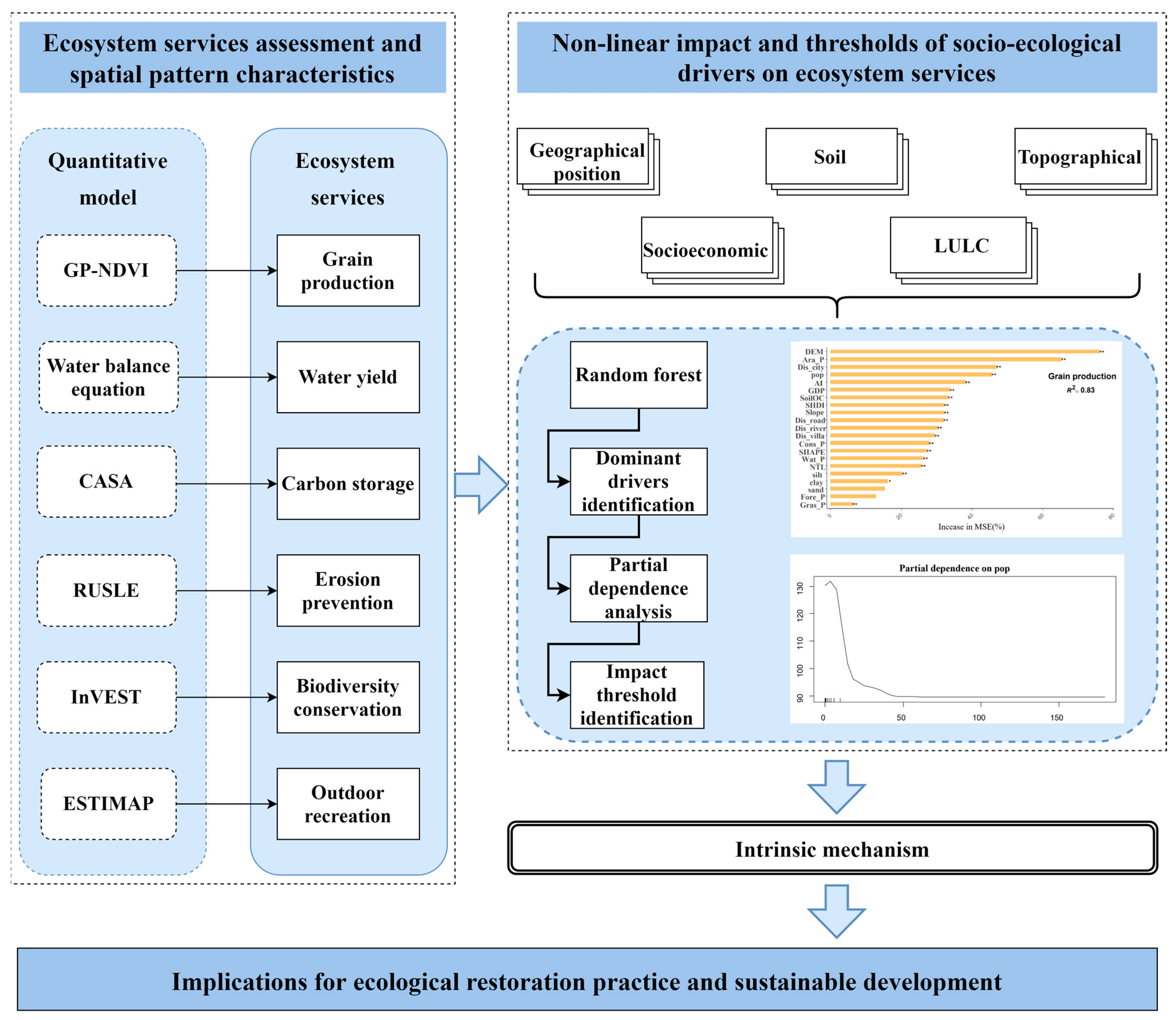
This study adopts a four-step analytical framework (Figure 2) to investigate non-linear impacts and thresholds of socio-ecological drivers on ESs: (1) Six ES indicators representing four major ES categories were quantified using various ecological models. (2) Socio-ecological drivers were selected across five socio-ecological dimensions. (3) Dominant socio-ecological drivers and their relative importance were identified via random forest. (4) Non-linear relationships and thresholds of dominant drivers on ESs were determined through partial dependence analysis. This approach aims to inform ES enhancement and regulation strategies.
All data were standardized to a 1 km grid spatial unit prior to analysis using ArcGIS’s Fishnet tool and Zonal Statistics functions. This resolution selection was based on the following: (1) It is the most accessible scale at which certain data, such as GDP and POP, can be obtained. (2) Analyzing the data at this scale allows for the reflection of the relationships between ESs and their drivers at a local level, while minimizing the computing burden at finer scales.

2.4. Selecting and Evaluating Ecosystem Services

Six ES indicators were selected as the study subject: grain production, water yield, carbon storage, erosion prevention, biodiversity conservation, and outdoor recreation. They were chosen because (1) they cover the supply services, regulating services, supporting services, and cultural services categories listed by MA (2005); (2) they are easily affected by various human activities; and (3) they can be conveniently assessed using existing models and methods, and the necessary data is readily available in the study area.
The six ES indicators were evaluated as follows: (1) Grain production was evaluated based on the relationship between grain production and NDVI index [26]. (2) Water yield service was assessed using a water balance equation, which considers that the amount of water produced by an ecosystem is influenced by precipitation and evapotranspiration [27]. (3) Carbon storage was calculated using NPP as a proxy variable based on the Carnegie–Ames–Stanford Approach (CASA) model, which calculates NPP as the product of photosynthesis active radiation absorbed by vegetation and an energy utilization efficiency. (4) Erosion prevention was evaluated using the revised universal soil loss equation (RUSLE) model [28]. (5) Biodiversity conservation was assessed through the habitat quality module of the InVEST model [29]. (6) Cultural services represent the non-material benefits that people derive from ecosystems, such as psychological enrichment and recreational enjoyment. We select outdoor recreation as a quantifiable proxy of cultural services, given its direct linkage to landscape accessibility and visitor engagement. Outdoor recreation was evaluated using the ESTIMAP-recreation method, which considers the degree of naturalness, natural protection, and presence of water as the major components contributing to the ability of a natural ecosystem to provide cultural service [4]. Under this methodology, outdoor recreation capacity exhibits an inverse relationship with anthropogenic landscape disturbance; protected areas are thus assigned high outdoor recreation capacity values, while water bodies contribute spatially extended recreational attractiveness to adjacent zones. For more information on the evaluation methods, please refer to the research of Zhang et al. [30].

2.5. Selecting Socio-Ecological Drivers on Ecosystem Services

ESs are influenced by various factors from natural and socio-economic aspects. Natural environment changes, such as topography and landforms, have an impact on the elements and structure of ecosystems, which in turn affects their capacity to provide various ESs. Specifically, topographic features—elevation, slope, and aspect—govern ES provision by regulating water drainage, shaping microclimates, and mediating habitat connectivity [31]. Land is the most important carrying basis of ecological process; thus, land use composition and landscape pattern also impact ESs like habitat quality, carbon sequestration services, and water conservation services [32,33]. Additionally, the physical and chemical properties of soil can regulate ESs by affecting biological growth and crop yields [34]. Furthermore, socio-economic development is often regarded as an indirect driver of ESs, which works by influencing human activities and environmental pollution [35]. Urbanization, accompanied by population growth and increased urban land use, transforms natural ecosystems into human-dominated or human-natural coupled ecosystems, which in turn influences a range of ESs [30]. Additionally, engineering projects such as infrastructural development, forestry plantation, and reforestation can also lead to changes in ESs directly or indirectly [12].
Based on the above considerations, 21 socio-ecological drivers were selected across five domains (terrain, soil, location, socio-economics, and land use) to analyze Ess’ driving mechanisms in Wuhan. The selection criteria included (1) relevance to local geographical conditions, (2) representation of key socio-ecological system components, and (3) data availability within the study area (Table 2). All data were standardized to a 1 km grid. Landscape metrics (Shape Index, Aggregation Index, and Shannon’s Diversity Index) were computed at the landscape level using Fragstats (https://www.fragstats.org/, accessed on 9 September 2025). Continuous variables (ES indicators, slope, and GDP) were aggregated by mean values via ArcGIS Zonal Statistics (https://pro.arcgis.com/en/pro-app/3.3/tool-reference/spatial-analyst/zonal-statistics.htm, accessed on 9 September 2025). Land use composition was calculated using ArcGIS Tabulate Area (https://pro.arcgis.com/en/pro-app/3.4/tool-reference/spatial-analyst/tabulate-area.htm, accessed on 9 September 2025). All the data was then imported into the R platform (https://www.r-project.org/, accessed on 9 September 2025) to conduct random forest modeling and partial dependence calculation using the RandomForest and rfPermute packages, respectively.

2.6. Quantifying Impacts and Thresholds of Socio-Ecological Drivers on Ecosystem Services

2.6.1. Identifying Dominant Socio-Ecological Drivers on Ecological Services

This study utilized a random forest model to quantify the degree of relative importance of various socio-ecological drivers on ESs and further identify the dominant drivers of ESs—defined as the top five drivers by importance ranking. Random forest is a non-parametric machine learning method that uses decision trees as base classifiers. Combining multiple independent decision trees and using the Bagging ensemble method, it obtains the final result [36].
There were mainly two important indicators to measure the importance of independent variables in random forest models: the increase in node purity (IncNodePurity) based on the Gimi index and the increase in mean squared error (%IncMSE) based on Out of Bag (OOB). The latter is a more commonly used metric, which utilizes the change in the mean squared error of OOB before and after the permutation of an independent variable to measure its degree of importance of it. The larger the %IncMSE, the higher the importance of the independent variable. The specific formula is as follows:
% I n c M S E i = j = 1 n ( e r r O O B 2 i j     e r r O O B 1 i j ) n
In the formula, % I n c M S E i is the increase in mean squared error of feature variable i . n is the number of occurrences of feature variable i in the forest. e r r O O B 1 i j is the error of OOB before randomly permuting the value of feature variable i . e r r O O B 2 i j is the error of OOB after randomly permuting the value of feature variable i . If the prediction error of OOB increases significantly after randomly permuting the value of feature variable   i , it indicates that the feature variable i has a great impact on the prediction results, i.e., the feature value has a high degree of importance. This study utilized the Random Forest package and the rfPermute package in R software to perform random forest modeling.

2.6.2. Quantifying Non-Linear Impacts and Thresholds of Dominant Socio-Ecological Drivers on Ecosystem Services

While random forest modeling effectively quantifies drivers’ importance, it fails to characterize intrinsic non-linear relationships between ESs and their drivers. To bridge this gap, this study employed partial dependence analysis to explore the non-linear impacts of dominant drivers on ESs and identify the corresponding impact thresholds. Partial dependency analysis is an explainable machine learning algorithm that can reveal the marginal effect of one or two features on the modeling outcome by marginalizing the influence of other features [37]. Compared to traditional regression models and mathematical statistical methods, partial dependency analysis can better explain the complex non-linear impacts of feature variables on dependent variables, visualize these relationships, and identify the impact thresholds, thus having the advantages of wide applicability and clear results. The specific calculation formula is as follows:
f ^ x s x s = 1 n i = 1 n f ^ ( x s , x c ( i ) )
In the formula, f ^ x s x s is the average impact of the targeted feature variable x s on the modeling outcome, x c is the other variables except for x s in the function, and n is the number of samples in the dataset. Partial dependence analysis was conducted in RStudio4.3.2, focusing exclusively on the top five drivers by importance ranking, as identified through random forest modeling.

3. Results

3.1. Spatial Distributions of Ecosystem Services

Spatial patterns of ESs in Wuhan are shown in Figure 3. Overall, except for soil conservation services, all the other ESs exhibited significant spatial differentiation, with low values gathered in the center and high values in the surroundings.
Specifically, the range of values for grain production service was 0–3.74 × 10⁷ kg. The high values were mostly found in the surrounding areas of city, where there was more clustered and contiguous basic arable land with good farming conditions. On the contrary, due to the scarcity of arable land resources, grain production services in urban central areas were correspondingly lower. The range of water yield service values was 1.96 × 10⁶–2.79 × 108 mm, showing the characteristic of “higher in the south than in the north, higher in the east than in the west, and higher in the surroundings than in the center”. The high-value areas for carbon storage service were mainly concentrated in the northwest Mulan Mountain area, the northeast Jiangjun Mountain area, and the southeast, while the low value areas were mainly located in the inner city. The value range of soil conservation service was 0–333.02 t/ha. The high value areas were mainly concentrated in the northern mountainous areas of Huangpi District, the Dabie Mountains in the northeast of Xinzhou District, and the southern and southwestern parts, while the service level in other areas was relatively low. High-value areas for biodiversity conservation services were mainly located around the city, accounting for more than 50% of the regional area, while low-level areas were mainly distributed in the central part of the city. The high-value areas for outdoor recreation service were mainly concentrated in the northwest, northeast, and south of the region, where natural ecosystems have a high cultural supply capacity due to their rich natural landscape resources and cultural relics. Owing to the presence of numerous parks and scenic spots within the urban area of Wuhan, there were also high-value areas for outdoor recreation service within and around the city. On the contrary, regions with the lowest outdoor recreation values were mainly concentrated in Jianghan District and Jiang’an District, which may be related to the high level of urbanization and industrialization in these areas, leading to a relative scarcity of natural resources.

3.2. Dominant Socio-Ecological Drivers on Ecosystem Services

The modeling results on the relative importance of various socio-ecological drivers on ESs are shown in Figure 4. The model ranks drivers based on their influence on ESs. Permutation tests assess the statistical significance of this ranking and the model’s overall goodness-of-fit. We can see that all the services have a fitting degree exceeding 80%, indicating that the model can fit the relationship between ESs and their drivers well. The dominant drivers of grain production services were DEM (elevation), Ara_P (proportion of arable land), Dis_city (distance from cities), POP (population density), and AI (aggregation index). The dominant drivers of water yield service were DEM (elevation), GDP (gross domestic product), Cons_P (proportion of construction land), SHDI (Shannon diversity index), and POP (population density). The dominant drivers of carbon storage service were AI (aggregation index), Dis_river (distance from rivers), Ara_P (proportion of arable land), Cons_P (proportion of construction land), and SHAPE (average shape index). The dominant drivers of soil conservation services are slope, DEM (elevation), Fore_P (proportion of forest land), Dis_city (distance from cities), and Dis_villa (distance from villages). The dominant drivers of biodiversity conservation services were AI (aggregation index), Ara_P (proportion of arable land), Fore_P (proportion of forest land), Cons_P (proportion of construction land), and SHAPE (average shape index). The dominant drivers of outdoor recreation service were Fore_P (proportion of forest land), Dis_river (distance from rivers), Dis_city (distance from cities), SHAPE (average shape index), and Ara_P (proportion of arable land).
Overall, Dis_river (distance from rivers), SoilOC (soil organic carbon content), SHDI (Shannon diversity index), and AI (aggregation index) had the most significant impacts on most ESs, followed by DEM (elevation), Fore_P (proportion of forest land), Cons_P (proportion of construction land), and Ara_P (proportion of arable land), while Gras_P (proportion of grassland), Clay (clay content), and Silt (silt content) appeared to have the least impact on the selected ESs.

3.3. Non-Linear Impacts and Thresholds of Dominant Socio-Ecological Drivers on Ecosystem Services

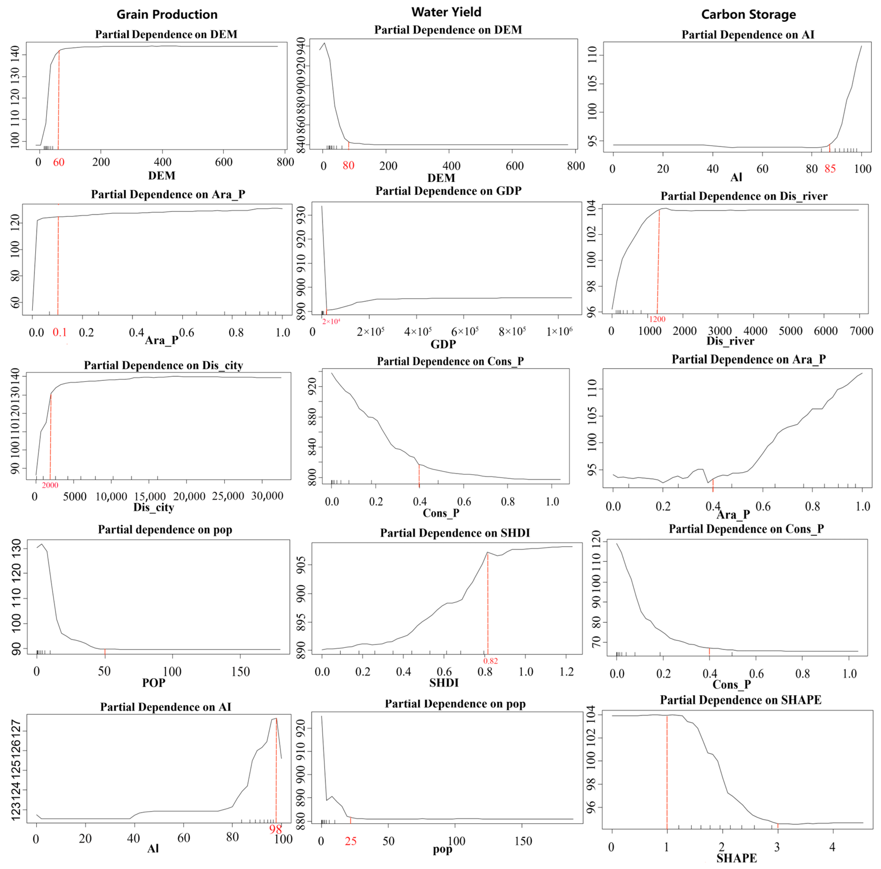
Figure 5 and Figure 6 present partial dependence plots, revealing three characteristic response patterns of ESs to dominant drivers: (1) single-threshold effects (predominant in most drivers), where ESs undergo abrupt changes when driver values exceed critical levels; (2) monotonic effects, with ESs consistently rising (monotonically increasing) or falling (monotonically decreasing) in response to driver variations without threshold behavior; and (3) complex non-linear effects (e.g., S-shaped, inverted S-shaped, and inverted U-shaped curves), typified by non-uniform response dynamics—S-shaped curves show gradual-then-accelerated ES shifts, inverted S-shapes exhibit rapid initial changes converging to stabilization, and inverted U-shapes peak at intermediate driver values before progressively declining.
Grain production service responds positively to increases in DEM (elevation), Ara_P (arable land proportion), and Dis_city (distance from cities), stabilizing beyond critical thresholds of 60 m, 10%, and 2000 m, respectively. Conversely, it declines with rising POP (population density) before stabilizing at low levels when POP exceeds 50 people/km2. AI (aggregation index) drives complex non-linear dynamics: service increases abruptly at AI = 80 but collapses sharply at AI = 98.
Water yield service had significant negative correlations with DEM (elevation), GDP (gross domestic product), Cons_P (proportion of construction land), and POP (population density), with thresholds of 80 m, 2 × 10⁴ million yuan, 0.4, and 25 people/km2, respectively. Beyond these thresholds, the decreasing trend of water yield services stabilized. In contrast, a positive correlation existed between water yield and SHDI (Shannon diversity index), with a threshold of 0.8.
The effects of AI (aggregation index) and Ara_P (arable land proportion) on carbon storage followed similar patterns: both services remained relatively low until thresholds of 85% (AI) and 40% (Ara_P) were reached, beyond which carbon storage increased dramatically. Carbon storage rose with increasing distance from rivers (Dis_river), plateauing when distance exceeded 1200 m. Conversely, higher Cons_P (construction land proportion) initially reduced carbon storage. After Cons_P surpassed 40%, the service stabilized at consistently low levels. The relationship between average shape index (SHAPE) and carbon storage exhibited an inverted S-shape: storage declined when SHAPE exceeded 1, with this trend stabilizing as SHAPE approached 3.
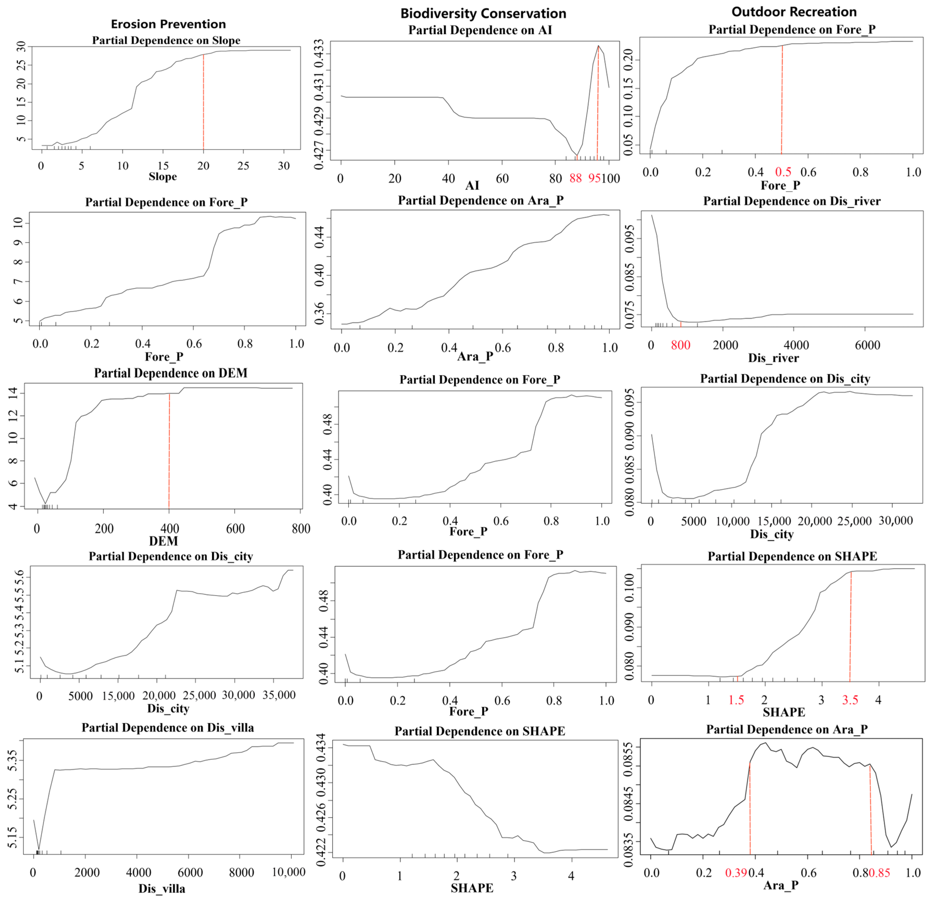
Erosion prevention services exhibited positive correlations with most dominant drivers, with thresholds of 20° and 400 m for Slope and DEM (elevation), respectively, and no significant thresholds for the remaining drivers. Biodiversity conservation services showed positive correlations with Ara_P (proportion of arable land) and Fore_P (proportion of forest land) but negative correlations with Cons_P (proportion of construction land) and SHAPE (average shape index).
Biodiversity conservation services displayed “monotonically increasing” correlations with Ara_P (proportion of arable land) and Fore_P (proportion of forest land). In contrast, its association with the AI (aggregation Index) exhibited complex non-linear dynamics: the service decreased incrementally until AI reached approximately 88 and then rose rapidly until AI approached 95, before undergoing an abrupt decline thereafter.
Outdoor recreation service had a positive correlation with Fore_P (proportion of forest land), with a threshold of 5%, and a negative connection with Dis_river (distance from rivers), with a threshold of 800 m. Furthermore, the service exhibited an “inverted S-shape” relationship with SHAPE (average shape index), staying relatively low when SHAPE is less than 1.5, then increasing rapidly until SHAPE reaches 3.5, and finally stabilizing at a relatively high level. The service exhibited an inverted U-shaped relationship with arable land proportion (Ara_P), maintaining high levels within the 39–85% range and low levels outside this interval. There was also a complex non-linear relationship between outdoor recreation service and Dis_city (distance from cities).

4. Discussion

4.1. Understanding the Non-Linear Impacts of Socio-Ecological Drivers on Ecosystem Services from a Threshold Perspective

Researchers and decision makers in ecological conservation and restoration are grappling with the question of what the primary factors are that determine ESs. However, finding a definite answer to this question is challenging, as it may vary depending on the research area [38], investigation method [21,39,40], and spatial scale of analysis [31,41]. Our study in Wuhan City found that natural conditions have a greater impact on ES distribution compared to human activities. The drivers of DEM, slope, Dis_river, and SoilOC were identified as the major determinants of most ESs. This suggests that while human activities can affect ESs, natural conditions remain the foundation of ecological structure and functions. Notably, this finding is inconsistent with that of Wang et al. [42], who found that ESs were more impacted by human disturbances in the Yellow River Basin. The difference may be attributed to factors such as climate conditions, water resources, and socio-economic development modes in the two study areas. Specifically, Wuhan belongs to the north subtropical monsoon humid climate, with abundant rainfall and water bodies covering the land surface, which has a favorable impact on various services such as food production, water yield, and carbon storage [43]. Although the Yellow River Basin also has abundant water, the availability and quality of its water resources face greater constraints, likely due to economic development and human activities [44]. Regarding socio-economic development mode, the Yellow River Basin may prioritize industrialization and urbanization, whereas Wuhan City places greater emphasis on ecological protection and sustainable development. While ESs in both regions are affected by human activities, the impact is more pronounced in the Yellow River Basin due to its historical agricultural development and recent industrialization. In addition, our research found that land use and land cover (LULC) factors, such as Fore_P and Cons_P, as well as the landscape pattern formed by different combinations of LULC types, were major determinants of ESs, consistent with the findings of Wen et al. [45] and Yee et al. [46]. This may be due to the fact that LULC change often leads to significant changes in the composition of ecosystems and their ability to provide various ESs.
The impact of socio-ecological drivers on ESs can be decomposed into three components—impact direction, impact magnitude, and threshold effect—as demonstrated by previous studies [47,48]. Despite the extensive research on the non-linear impact mechanism, there is a lack of studies summarizing the curve characteristics and threshold types of this impact. In our study, we categorized the non-linear impacts of socio-ecological drivers on ESs from a threshold perspective into three types: “single threshold”, “monotonic impact”, and “complex curve” effects.
The “single threshold” effect is a phenomenon that demonstrates when a driver’s value reaches a certain level, its impact on ESs becomes stable. Taking the effect of Dis_river on outdoor recreation service for an example, the service decreased with increasing distance from the rivers until the distance increased to 1000 m. This can be attributed to rivers being significant natural landscapes with great tourism and recreational appeal [4]. As the distance from the rivers increases, the convenience for people to engage in outdoor activities using the water (such as swimming, fishing, and boating) decreases, resulting in fewer people willing to participate in water-related activities beyond 1000 m.
The “monotonic impact” effect depicts a relationship that ESs are continuously promoted or inhibited as a specific driver increases, without exhibiting any threshold effect. This effect can be easily observed in the relationship between Cons_P and water yield, carbon storage, and biodiversity conservation services. These services steadily decrease as Cons_P increases, presenting a “monotonically diminishing” curve pattern. Similar findings have been reported in previous research [49,50,51]. The primary reason for this is that an increase in construction land can cause the natural surface to impermeable surface, preventing precipitation from effectively infiltrating the ground. This, in turn, leads to a rapid loss of precipitation in the form of surface runoff, reducing water yield services. Additionally, the transformation from natural surface to impermeable surface also results in a decrease in vegetation cover and creates physical barriers that impede species migration and gene flow. This increases ecological isolation, decreases carbon storage services, and endangers biodiversity.
The “complex curve” effect manifests a curve characteristic of positive and negative effects intersected or mixed with each other, that is, drivers have a positive impact on ESs within a certain range of values, while in another range of values, their impact on ESs is negative; meanwhile, these positive and negative effects are intersected. The “complex curve” effect could be embodied into “S-shape”, “inverted S-shape”, and “inverted U-shape” effects. Taking the “S-shape” effect of SHAPE on outdoor recreation service as an example, when SHDI remains at a relatively low value, as the SHDI increased, the service stabilizes at a low level; when the SHDI hits a certain value, the service increases sharply; when the SHDI reaches another value, the service stays at a high level again. This may be because a higher SHDI value signifies a more complex and heterogeneous landscape [52] and thus indicates more attractiveness for people to participate in outdoor recreation. When SHDI remains at a lower level, the capacity of landscape to attract people stays relatively low, but when SHDI reaches a certain threshold, an increase in landscape complexity would greatly increase the willingness of people to visit and recreate outdoor. However, when the SHDI reaches another high level, the capacity of landscape to provide outdoor recreation would not be continuously promoted because it has already attracted most people around.

4.2. Policy Implications for Ecological Restoration

Ecological restoration is a crucial activity that improves ecosystem functions and restore ecosystem health and stability by repairing ecosystems that are structurally disordered, functionally impaired, or even damaged [53]. Accurately identifying ecological restoration areas is a crucial issue in ecological restoration activities, and many studies have identified areas with low ES values, ecologically sensitive areas, and ecological inflection points as potential ecological restoration areas [14,54]. Once ecological restoration areas are identified, selecting appropriate ecological restoration measures becomes a challenging problem for urban planners. Previous studies have primarily selected restoration measures based on an analysis of the background conditions, major problems, and target tasks, without quantitatively analyzing the impact mechanisms and thresholds of drivers on ESs [55,56]. By quantitatively analyzing the impact mechanisms and thresholds of drivers on ESs, it is possible to select ecological restoration measures in a more scientifical and reasonable manner, thereby enhancing the capacity of ESs.
Based on our research, the dominant drivers and their impact directions varied across different ESs. When faced with the degradation of ESs caused by various socio-ecological drivers, managers can firstly identify areas of ES decline or low value and then take targeted restoration measures to address the dominant drivers according to the findings in Section 4.2 to influence the targeted ESs. For example, AI, Dis_river, Ara_P, Cons_P, and SHAPE were found to be the major determinants of carbon storage service. The proportion of Ara_P, Dis_river, and AI all increased the capacity of carbon storage service, while the Cons_P and SHAPE decreased it. Therefore, in areas where carbon storage degradation is severe, particularly in urban centers and at the edge of basic arable land protection zones, measures such as adding water sources, cultivating arable land, planting trees, and optimizing land use layout (e.g., increasing the degree of land-use agglomeration and regularizing land patches) can be taken to restore the carbon storage service. For degraded areas that provide multiple ESs, comprehensive steps should be undertaken to improve the overall capacity of ecosystems to provide various ESs.
However, our research demonstrated that the impacts of most socio-ecological drivers on ESs had significant threshold effects; that is, once the value of a driver exceeds a specific threshold, its impact on ESs would change dramatically. This is consistent with the findings of Peng et al. [20], Zhao et al. [57], and Wang et al. [58]. In order to “achieve greater returns with smaller inputs”, we should control ecological restoration efforts within a predetermined threshold. Water yield service, for instance, was found to rise with the area percentage of water bodies. However, this growth stabilized at a percentage of water area greater than 0.4. This implies that maintaining the water area share within 0.4 will maximize the impact of an increase in water yield service, while going above that will drastically lower the desired effect.

4.3. Limitations and Prospects

Compared to previous methods such as correlation analysis [59,60], Geodetector [61,62], and geographically weighted regression [63], the random forest utilized in this study has a significant advantage in dealing with complex socio-ecological data. It can effectively evaluate interactions among various drivers and quantify their relative importance on ESs. Furthermore, the partial dependency analysis can depict the curvilinear impacts of dominant drivers on ESs and identify the impact thresholds from a global perspective. Based on this, we were able to summarize three types of non-linear impacts of socio-ecological drivers on ESs from a threshold perspective, which is a novel contribution to the field. Moreover, compared to previous studies that have focused on administrative scales [58], the 1 km grid cell utilized in this study allows for a clearer demonstration of the interactions between ESs and their drivers in local space. This provides more detailed guidance for the selection of measures for ecological restoration.
This study has several limitations in addition to the aforementioned advancements. First, the analyses of mechanisms affecting ESs in this paper were conducted at a single scale, but scale effects exist in the driven mechanisms of ESs due to the intricate and hierarchical structure of ecosystems [64]. Ignoring these effects may bias the results, so further research at various scales is necessary to understand how stable the relationship is. Second, this work did not take human and policy factors into much account in the selection of socio-ecological drivers [65]. In the future, a more thorough understanding of the internal mechanism of ESs could be achieved by developing a better framework for drivers.

5. Conclusions

This study investigated the non-linear impacts of socio-ecological drivers on ESs from a threshold perspective. Key findings revealed significant spatial heterogeneity for most ESs in Wuhan (excluding erosion prevention service), manifesting as a distinct “low central, high peripheral” pattern. Among all the socio-ecological drivers, DEM, Dis_river, SoilOC, AI, and SHDI emerged as the most influential on ES provision, whereas grassland percentage and soil texture components (sand, silt, and clay) were the least important. Furthermore, threshold analysis identified three distinct types of non-linear relationships between ESs and their drivers: (1) “Single threshold” effects were predominated for most drivers. (2) Monotonic impacts (“monotonically increasing” or “monotonically decreasing”) were characterized for a minority of drivers. (3) Complex curve effects (e.g., “S-shape”, “inverted S-shape”, and “inverted U-shape”) were observed for the remaining drivers. In practice, decision-makers can implement targeted restoration measures to address key drivers, thereby enhancing the delivery of specific ESs. Furthermore, restoration efforts should be kept within optimal thresholds to maximize outcomes with minimal inputs. This study offers valuable insights for improving ES provision and supporting sustainable development strategies.

Author Contributions

Conceptualization, Y.Z. and Y.C.; methodology, S.L.; software, S.L.; validation, H.L. and Y.C.; formal analysis, S.L.; investigation, Y.Z.; resources, Y.Z. and Y.C.; data curation, H.L., F.K., and Y.Z.; writing—original draft preparation, Y.Z. and S.L.; writing—review and editing, P.Y. and Y.C.; visualization, S.L.; supervision, G.J. and Y.C.; project administration, Y.Z. and Y.C.; funding acquisition, Y.Z. and G.J. All authors have read and agreed to the published version of the manuscript.

Funding

This study was financially supported by the National Natural Science Foundation of China (No. 42101284 and No.71974070).

Data Availability Statement

The data presented in this study are available from the corresponding author on reasonable request. The data are not publicly available due to privacy policies.

Conflicts of Interest

The authors declare no conflicts of interest.

References

  1. Costanza, R.; D’Arge, R.; Groot, R.D.; Farber, S.; Grasso, M.; Hannon, B.; Limburg, K.; Naeem, S.; O’Neill, R.V.; Paruelo, J. The value of the world’s ecosystem services and natural capital. Ecol. Econ. 1997, 25, 3–15. [Google Scholar] [CrossRef]
  2. Bridgewater, P.; Schmeller, D.S. The Ninth Plenary of the Intergovernmental Platform on Biodiversity and Ecosystem Services (IPBES-9): Sustainable use, values, and business (as usual). Biodivers. Conserv. 2023, 32, 1–6. [Google Scholar] [CrossRef] [PubMed]
  3. Burkhard, B.; Kandziora, M.; Hou, Y.; Müller, F. Ecosystem service potentials, flows and demands-concepts for spatial localisation, indication and quantification. Landsc. Online 2014, 34, 1–32. [Google Scholar] [CrossRef]
  4. Baró, F.; Palomo, I.; Zulian, G.; Vizcaino, P.; Haase, D.; Gómez-Baggethun, E. Mapping ecosystem service capacity, flow and demand for landscape and urban planning: A case study in the Barcelona metropolitan region. Land Use Policy 2016, 57, 405–417. [Google Scholar] [CrossRef]
  5. Li, C.; Qiao, W.; Gao, B.; Chen, Y. Unveiling spatial heterogeneity of ecosystem services and their drivers in varied landform types: Insights from the Sichuan-Yunnan ecological barrier area. J. Clean. Prod. 2024, 442, 141158. [Google Scholar] [CrossRef]
  6. Shifaw, E.; Sha, J.; Li, X.; Bao, Z.; Ji, J.; Ji, Z.; Kassaye, A.Y.; Lai, S.; Yang, Y. Ecosystem services dynamics and their influencing factors: Synergies/ tradeoffs interactions and implications, the case of upper Blue Nile basin, Ethiopia. Sci. Total Environ. 2024, 938, 173524. [Google Scholar] [CrossRef]
  7. Mirghaed, F.A.; Mohammadzadeh, M.; Salmanmahiny, A.; Mirkarimi, S.H. Decision scenarios using ecosystem services for land allocation optimization across Gharehsoo watershed in northern Iran. Ecol. Indic. 2020, 117, 106645. [Google Scholar] [CrossRef]
  8. Peng, J.; Yang, Y.; Liu, Y.X.; Hu, Y.N.; Du, Y.Y.; Meersmans, J.; Qiu, S.J. Linking ecosystem services and circuit theory to identify ecological security patterns. Sci. Total Environ. 2018, 644, 781–790. [Google Scholar] [CrossRef]
  9. Deng, H.W.; Zhou, X.F.; Liao, Z.L. Ecological redline delineation based on the supply and demand of ecosystem services. Land Use Policy 2024, 140, 107109. [Google Scholar] [CrossRef]
  10. Kim, J.; Song, Y. Integrating ecosystem services and ecological connectivity to prioritize spatial conservation on Jeju Island, South Korea. Landsc. Urban Plan. 2023, 239, 104865. [Google Scholar] [CrossRef]
  11. Gissi, E.; Manea, E.; Mazaris, A.D.; Fraschetti, S.; Almpanidou, V.; Bevilacqua, S.; Coll, M.; Guarnieri, G.; Lloret-Lloret, E.; Pascual, M.; et al. A review of the combined effects of climate change and other local human stressors on the marine environment. Sci. Total Environ. 2021, 755, 142564. [Google Scholar] [CrossRef]
  12. Helseth, E.V.; Vedeld, P.; Framstad, E.; Gómez-Baggethun, E. Forest ecosystem services in Norway: Trends, condition, and drivers of change (1950–2020). Ecosyst. Serv. 2022, 58, 101491. [Google Scholar] [CrossRef]
  13. Guo, M.; Ma, S.; Wang, L.-J.; Lin, C. Impacts of future climate change and different management scenarios on water-related ecosystem services: A case study in the Jianghuai ecological economic Zone, China. Ecol. Indic. 2021, 127, 107732. [Google Scholar] [CrossRef]
  14. Hu, M.; Zhang, H.; Tang, J.; Yan, S. Zoning and Optimization Strategies of Land Spatial Ecological Restoration in Liangjiang New Area of Chongqing Based on the Supply–Demand Relationship of Ecosystem Services. Land 2023, 12, 1255. [Google Scholar] [CrossRef]
  15. Ngabire, M.; Wang, T.; Xue, X.; Liao, J.; Sahbeni, G.; Huang, C.; Duan, H.; Song, X. Soil salinization mapping across different sandy land-cover types in the Shiyang River Basin: A remote sensing and multiple linear regression approach. Remote Sens. Appl. Soc. Environ. 2022, 28, 100847. [Google Scholar] [CrossRef]
  16. Mouchet, M.A.; Paracchini, M.L.; Schulp, C.J.E.; Stürck, J.; Verkerk, P.J.; Verburg, P.H.; Lavorel, S. Bundles of ecosystem (dis)services and multifunctionality across European landscapes. Ecol. Indic. 2017, 73, 23–28. [Google Scholar] [CrossRef]
  17. Hu, B.; Kang, F.; Han, H.; Cheng, X.; Li, Z. Exploring drivers of ecosystem services variation from a geospatial perspective: Insights from China’s Shanxi Province. Ecol. Indic. 2021, 131, 108188. [Google Scholar] [CrossRef]
  18. Kang, J.; Li, C.; Zhang, B.; Zhang, J.; Li, M.; Hu, Y. How do natural and human factors influence ecosystem services changing? A case study in two most developed regions of China. Ecol. Indic. 2023, 146, 109891. [Google Scholar] [CrossRef]
  19. Geng, J.; Yuan, M.; Xu, S.; Bai, T.; Xiao, Y.; Li, X.; Xu, D. Urban Expansion Was the Main Driving Force for the Decline in Ecosystem Services in Hainan Island during 1980–2015. Int. J. Environ. Res. Public Health 2022, 19, 15665. [Google Scholar] [CrossRef] [PubMed]
  20. Peng, J.; Tian, L.; Liu, Y.; Zhao, M.; Hu, Y.; Wu, J. Ecosystem services response to urbanization in metropolitan areas: Thresholds identification. Sci. Total Environ. 2017, 607, 706–714. [Google Scholar] [CrossRef]
  21. Sun, X.; Tang, H.; Yang, P.; Hu, G.; Liu, Z.; Wu, J. Spatiotemporal patterns and drivers of ecosystem service supply and demand across the conterminous United States: A multiscale analysis. Sci. Total Environ. 2020, 703, 135005. [Google Scholar]
  22. Olaniyi, O.E.; Omowale, H.O. Evaluating the dynamics and eco-climatic predictors of forest conversion and restoration in Old Oyo National Park, Nigeria using geospatial and machine learning techniques. Model. Earth Syst. Environ. 2022, 8, 227–244. [Google Scholar]
  23. Lin, Y.; Lee, D. Changes in land use or land cover and ecosystem service values in Wuhan city, China, from 1996 to 2018. J. Chin. Archit. Urban. 2023, 5, 0427. [Google Scholar]
  24. Han, P.; Hu, H.; Zhou, J.; Wang, M.; Zhou, Z. Integrating key ecosystem services to study the spatio-temporal dynamics and determinants of ecosystem health in Wuhan’s central urban área. Ecol. Indic. 2024, 166, 112352. [Google Scholar]
  25. Zhu, J.; Ke, X.; Zhou, T.; He, L. Evaluation of ecological security of natural resources in Wuhan based on “contribution, vitality, organisational strength and resilience”. Bull. Soil Water Conserv. 2023, 43, 248–255. [Google Scholar]
  26. Cao, Y.; Li, G.; Tian, Y.; Fang, X.; Li, Y.; Tan, Y. Linking ecosystem services trade-offs, bundles and hotspot identification with cropland management in the coastal Hangzhou Bay area of China. Land Use Policy 2020, 97, 104689. [Google Scholar] [CrossRef]
  27. Jia, X.; Fu, B.; Feng, X.; Hou, G.; Liu, Y.; Wang, X. The tradeoff and synergy between ecosystem services in the Grain-for-Green areas in Northern Shaanxi, China. Ecol. Indic. 2014, 43, 103–113. [Google Scholar] [CrossRef]
  28. Rejani, R.; Rao, K.V.; Osman, M.; Rao, C.S.; Reddy, K.S.; Chary, G.R.; Pushpanjali; Samuel, J. Spatial and temporal estimation of soil loss for the sustainable management of a wet semi-arid watershed cluster. Environ. Monit. Assess. 2016, 188, 143. [Google Scholar] [CrossRef]
  29. Tallis, H.; Ricketts, T. InVEST 1.0 Beta User’s Guide: Integrated Valuation of Ecosystem Services and Tradeoffs; Woods Institute for the Environment, Stanford University: California, CA, USA, 2010. [Google Scholar]
  30. Zhang, Y.; Liu, Y.; Zhang, Y.; Liu, Y.; Zhang, G.; Chen, Y. On the spatial relationship between ecosystem services and urbanization: A case study in Wuhan, China. Sci. Total Environ. 2018, 637, 780–790. [Google Scholar]
  31. Ma, S.; Qiao, Y.-P.; Wang, L.-J.; Zhang, J.-C. Terrain gradient variations in ecosystem services of different vegetation types in mountainous regions: Vegetation resource conservation and sustainable development. For. Ecol. Manag. 2021, 482, 118856. [Google Scholar] [CrossRef]
  32. Clerici, N.; Cote-Navarro, F.; Escobedo, F.J.; Rubiano, K.; Villegas, J.C. Spatio-temporal and cumulative effects of land use-land cover and climate change on two ecosystem services in the Colombian Andes. Sci. Total Environ. 2019, 685, 1181–1192. [Google Scholar] [CrossRef]
  33. Liu, W.; Zhan, J.; Zhao, F.; Yan, H.; Zhang, F.; Wei, X. Impacts of urbanization-induced land-use changes on ecosystem services: A case study of the Pearl River Delta Metropolitan Region, China. Ecol. Indic. 2019, 98, 228–238. [Google Scholar] [CrossRef]
  34. Krawczynski, R.; Milne, E.; Banwart, S.A. Soil carbon, multiple benefits. J. Environ. Res. Dev. 2015, 13, 33–38. [Google Scholar]
  35. Reid, W.; Mooney, H.; Cropper, A.; Capistrano, D.; Carpenter, S.; Chopra, K. Millennium Ecosystem Assessment. Ecosystems and human well-being. Synthesis 2005, 34, 534. [Google Scholar]
  36. Breiman, L. Random Forests. Mach. Learn. 2001, 45, 5–32. [Google Scholar] [CrossRef]
  37. Parr, T.; Wilson, J.D. Partial dependence through stratification. Mach. Learn. Appl. 2021, 6, 100146. [Google Scholar] [CrossRef]
  38. Wang, Y.; Cai, Y.; Xie, Y.; Zhang, P.; Chen, L. Dissecting ecosystem services distribution and inequality of typical cities in China. J. Clean. Prod. 2023, 415, 137800. [Google Scholar] [CrossRef]
  39. Hou, W.; Hu, T.; Yang, L.; Liu, X.; Zheng, X.; Pan, H.; Zhang, X.; Xiao, S.; Deng, S. Matching ecosystem services supply and demand in China’s urban agglomerations for multiple-scale management. J. Clean. Prod. 2023, 420, 138351.1. [Google Scholar] [CrossRef]
  40. Shen, J.; Li, S.; Wang, H.; Wu, S.; Liang, Z.; Zhang, Y.; Wei, F.; Li, S.; Ma, L.; Wang, Y.; et al. Understanding the spatial relationships and drivers of ecosystem service supply-demand mismatches towards spatially-targeted management of social-ecological system. J. Clean. Prod. 2023, 406, 136882. [Google Scholar] [CrossRef]
  41. Xiong, C.; Ren, H.; Xu, D.; Gao, Y. Spatial scale effects on the value of ecosystem services in China’s terrestrial area. J. Environ. Manag. 2024, 366, 121745. [Google Scholar] [CrossRef]
  42. Wang, X.; Wang, B.; Cui, F. Exploring ecosystem services interactions in the dryland: Socio-ecological drivers and thresholds for better ecosystem management. Ecol. Indic. 2024, 159, 111699. [Google Scholar] [CrossRef]
  43. Cui, X.; Huang, L. Integrating ecosystem services and ecological risks for urban ecological zoning: A case study of Wuhan City, China. Hum. Ecol. Risk Assess. 2023, 29, 1299–1317. [Google Scholar] [CrossRef]
  44. Li, N.; Sun, P.; Zhang, J.; Mo, J.; Wang, K. Spatiotemporal evolution and driving factors of ecosystem services’ transformation in the Yellow River basin, China. Environ. Monit. Assess. 2024, 196, 252. [Google Scholar] [CrossRef]
  45. Wen, X.; Théau, J. Spatiotemporal analysis of water-related ecosystem services under ecological restoration scenarios: A case study in northern Shaanxi, China. Sci. Total Environ. 2020, 720, 137477. [Google Scholar] [CrossRef] [PubMed]
  46. Yee, S.H.; Paulukonis, E.; Simmons, C.; Russell, M.; Fulford, R.; Harwell, L.; Smith, L. Projecting effects of land use change on human well-being through changes in ecosystem services. Ecol. Model. 2021, 440, 109358. [Google Scholar] [CrossRef] [PubMed]
  47. He, L.; Xie, Z.; Wu, H.; Liu, Z.; Zheng, B.; Wan, W. Exploring the interrelations and driving factors among typical ecosystem services in the Yangtze river economic Belt, China. J. Environ. Manag. 2024, 351, 119794. [Google Scholar] [CrossRef]
  48. Huang, X.; Xie, Y.; Lei, F.; Cao, L.; Zeng, H. Analysis on spatio-temporal evolution and influencing factors of ecosystem service in the Changsha-Zhuzhou-Xiangtan urban agglomeration, China. Front. Environ. Sci. 2024, 11, 1334458. [Google Scholar] [CrossRef]
  49. Yi, J.; Dai, S.; Cheng, J.; Liu, K. How urban sprawl affects local and nearby ecosystem services in China. Reg. Environ. Change 2023, 23, 139. [Google Scholar] [CrossRef]
  50. Felipe-Lucia, M.; Soliveres, S.; Penone, C.; Fischer, M.; Ammer, C.; Boch, S.; Boeddinghaus, R.S.; Bonkowski, M.; Buscot, F.; Fiore-Donno, A.M.; et al. Land-use intensity alters networks between biodiversity, ecosystem functions, and services. Proc. Natl. Acad. Sci. USA 2020, 117, 28140–28149. [Google Scholar] [CrossRef]
  51. Wu, J.; Li, X.; Luo, Y.; Zhang, D. Spatiotemporal effects of urban sprawl on habitat quality in the Pearl River Delta from 1990 to 2018. Sci. Rep. 2021, 11, 13981. [Google Scholar] [CrossRef]
  52. Jiang, Y.; Ouyang, B.; Yan, Z. Multiscale Analysis for Identifying the Impact of Human and Natural Factors on Water-Related Ecosystem Services. Sustainability 2024, 16, 1738. [Google Scholar] [CrossRef]
  53. Fu, B.; Liu, Y.; Meadows, M.E. Ecological restoration for sustainable development in China. Natl. Sci. Rev. 2023, 10, nwad033. [Google Scholar] [CrossRef]
  54. Liu, Y.; Huang, J.; Lin, W. Zoning strategies for ecological restoration in the karst region of Guangdong province, China: A perspective from the “socio-ecological system”. Front. Environ. Sci. 2024, 12, 1369635. [Google Scholar] [CrossRef]
  55. Bian, H.; Li, M.; Deng, Y.; Zhang, Y.; Liu, Y.; Wang, Q.; Xie, S.; Wang, S.; Zhang, Z.; Wang, N. Identification of ecological restoration areas based on the ecological safety security assessment of wetland-hydrological ecological corridors: A case study of the Han River Basin in China. Ecol. Indic. 2024, 160, 111780. [Google Scholar] [CrossRef]
  56. Chen, W.; Gu, T.; Xiang, J.; Luo, T.; Zeng, J.; Yuan, Y. Ecological restoration zoning of territorial space in China: An ecosystem health perspective. J. Environ. Manag. 2024, 364, 121371. [Google Scholar] [CrossRef]
  57. Zhao, M.; Zhou, Q.; Luo, Y.; Li, Y.; Wang, Y.; Yuan, E. Threshold Effects between Ecosystem Services and Natural and Social Drivers in Karst Landscapes. Land 2024, 13, 691. [Google Scholar] [CrossRef]
  58. Wang, W.; Xu, J.; Luan, X.; Zhang, Z. Wetland ecosystem service values in Beijing significantly increased from 1984 to 2020: Trend changes, type evolution, and driving factor. Ecol. Indic. 2024, 166, 112235. [Google Scholar] [CrossRef]
  59. Bailey, R.G. Delineation of ecosystem regions. Environ. Manag. 1983, 7, 365–373. [Google Scholar] [CrossRef]
  60. Chen, X.; He, L.; Luo, F.; He, Z.; Bai, W.; Xiao, Y.; Wang, Z. Dynamic characteristics and impacts of ecosystem service values under land use change: A case study on the Zoigê plateau, China. Ecol. Inform. 2023, 78, 102350. [Google Scholar] [CrossRef]
  61. Sun, H.; Di, Z.; Sun, P.; Wang, X.; Liu, Z.; Zhang, W. Spatiotemporal Differentiation and Its Attribution of the Ecosystem Service Trade-Off/Synergy in the Yellow River Basin. Land 2024, 13, 369. [Google Scholar] [CrossRef]
  62. Wu, L.; Luo, Y.; Pang, S.; Wang, G.; Ma, X. Factor analysis of hydrologic services in water-controlled grassland ecosystems by InVEST model and geodetector. Environ. Sci. Pollut. Res. 2024, 31, 20409–20433. [Google Scholar] [CrossRef] [PubMed]
  63. Jia, K.; Huang, A.; Yin, X.; Yang, J.; Deng, L.; Lin, Z. Investigating the Impact of Urbanization on Water Ecosystem Services in the Dongjiang River Basin: A Spatial Analysis. Remote Sens. 2023, 15, 2265. [Google Scholar] [CrossRef]
  64. Zhang, X.; Han, R.; Yang, S.; Yang, Y.; Tang, X.; Qu, W. Identification of bundles and driving factors of ecosystem services at multiple scales in the eastern China region. Ecol. Indic. 2024, 158, 111378. [Google Scholar] [CrossRef]
  65. Chen, C.; Liu, Y. Spatiotemporal changes of ecosystem services value by incorporating planning policies: A case of the Pearl River Delta, China. Ecol. Model. 2021, 461, 109777. [Google Scholar] [CrossRef]
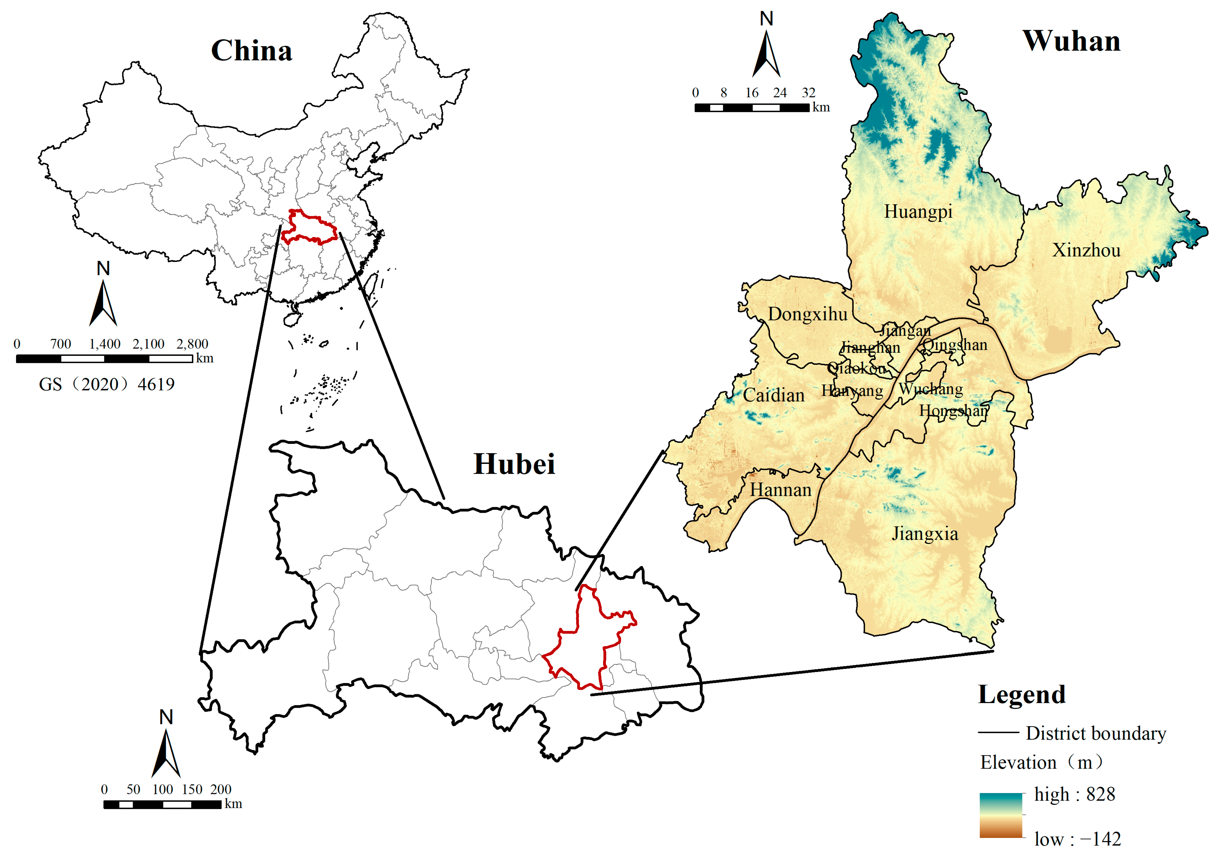
Figure 1. Location and elevation of Wuhan City.
Urbansci 09 00390 g001
Figure 2. Framework of the proposed method. *: p < 0.05; **: 0.05 ≤ p < 0.1.
Urbansci 09 00390 g002
Figure 3. Spatial patterns of ecosystem services in Wuhan.
Urbansci 09 00390 g003
Figure 4. Relative importances of socio-ecological drivers on ecosystem services. (*: p < 0.05; **: 0.05 ≤ p < 0.1).
Urbansci 09 00390 g004
Figure 5. Partial dependency plots on the impacts of dominant socio-ecological drivers on grain production (left), water yield (middle), and carbon storage (right) services.
Urbansci 09 00390 g005
Figure 6. Partial dependency plots on the impacts of dominant socio-ecological drivers on erosion prevention (left), biodiversity conservation (middle), and outdoor recreation services (right).
Urbansci 09 00390 g006
Table 1. Source of data utilized in this study.
CategoryDataDatesource
Physical geographic dataDigital Elevation Model
(DEM)
Geospatial Data Cloud GDEMV2 dataset (https://www.gscloud.cn/#page1/3, accessed on 28 January 2024)
Soil typeChina soil map based harmonised world soil data base (HWSD) (https://data.tpdc.ac.cn/zh-hans/, accessed on 30 January 2024)
PrecipitationNational Earth System Science Data Centre (http://www.geodata.cn/data/, accessed on 31 March 2024)
TemperatureNational Earth System Science Data Centre (http://www.geodata.cn/data/, accessed on 24 March 2024)
Solar radiationUnited States National Climatic Data Centre (https://www.ncei.noaa.gov/cdo-web/, accessed on 24 March 2024)
Leaf area indexNational Earth System Science Data Centre (http://www.geodata.cn/data/, accessed on 19 March 2024)
Normalized Difference Vegetation Index (NDVI)Geospatial Data Cloud Landsat 8, Resource and Environment Science and Data Centre (https://www.resdc.cn/Default.aspx, accessed on 24 March 2024)
VegetationResource and Environmental Science Data Platform (https://www.resdc.cn/Default.aspx, accessed on 23 March 2024)
Socio-economic dataAdministrative subdivisionResource and Environmental Science Data Platform (https://www.resdc.cn/Default.aspx, accessed on 24 January 2024)
Population density (POP)National Earth System Science Data Centre (http://www.geodata.cn/data/, accessed on 27 March 2024)
Gross domestic product
(GDP)
Geographic remote sensing ecological network platform (http://gisrs.cn/, accessed on 29 January 2024)
Night light dataNational Earth System Science Data Centre (http://www.geodata.cn/data/, accessed on 24 March 2024)
Land use/land coverResource and Environment Science and Data Centre (https://www.resdc.cn/Default.aspx, accessed on 26 January 2024)
China Land Cover DatasetNational Cryosphere Desert Data Centre (https://www.ncdc.ac.cn/portal/?lang=en&clear_cache=1, accessed on 28 January 2024)
Grain productionWuhan Statistical Yearbook (https://tjj.wuhan.gov.cn/tjfw/tjnj/, accessed on 27 January 2024)
Table 2. Indicators of socio-ecological drivers influencing ecosystem services.
ObjectiveCriteriaIndicatorEncoding
Indicator system for ESs impact factorsTopographicalElevationDEM
SlopeSlope
SoilClay contentClay
Silt contentSilt
Sand contentSand
Soil organic carbon contentSoilOC
Geographical positionDistance from citiesDis_city
Distance from villagesDis_villa
Distance from roadsDis_road
Distance from riversDis_river
Socio-economicPopulation densityPOP
Gross domestic productGDP
Nighttime Lighting IndexNTL
LULCProportion of arable landAra_P
Proportion of forest landFore_P
Proportion of grasslandGras_P
Proportion of construction landCons_P
Proportion of watersWat_P
Average shape indexSHAPE
Aggregation indexAI
Shannon diversity indexSHDI
Disclaimer/Publisher’s Note: The statements, opinions and data contained in all publications are solely those of the individual author(s) and contributor(s) and not of MDPI and/or the editor(s). MDPI and/or the editor(s) disclaim responsibility for any injury to people or property resulting from any ideas, methods, instructions or products referred to in the content.