Mitigation and Resilience of Local Climatic Zones to the Effects of Extreme Heat: Study on the City of Barcelona (Spain)

Abstract

Global warming is precipitating an amplification of severe meteorological occurrences such as prolonged dry spells and episodes of elevated temperatures. These phenomena are instigating substantial elevations in environmental warmth, with metropolitan regions bearing the brunt of these impacts. Currently, extreme heat is already impacting 30% of the global populace, and forecasts suggest that this figure will escalate to 74% in the forthcoming years. One of the objectives outlined in the United Nations 2030 agenda, specifically within Sustainable Development Goal 11 (SDG11), is the attainment of sustainable urban development. To achieve this, it is imperative to scrutinize and delve into urban environmental conditions in order to understand their dynamics comprehensively. This understanding serves as the foundation for implementing mitigation and resilience strategies against climate change, ultimately enhancing the well-being of city residents. In this context, the field of remote sensing and geographic information systems has made substantial advancements. Notably, the UrbClim model, developed by the European Space Agency, facilitates the assessment of environmental conditions within numerous European urban centers. This research, utilizing data from UrbClim, examines the evolution of the heat stress index (Hi) during extreme heat conditions in Barcelona during the summer of 2017. Leveraging Landsat 8 satellite imagery, we derived the following variables: the normalized difference vegetation index and the normalized building difference index. Our findings reveal that during extreme heat conditions, the Hi index experiences an escalation, with areas characterized by a higher population density and industrial zones displaying lower resistance in contrast to regions with a lower population density and rural areas, which exhibit greater resilience to Hi. This disparity can be attributed to higher vegetation coverage and reduced building density in the latter areas. In this way, Hi increases more quickly and intensely and decreases more slowly when using high temperatures compared to average temperatures. This is of utmost importance for the future planning of new urban developments.

1. Introduction

In recent decades, there has been a substantial rise in environmental temperatures, as confirmed by the Intergovernmental Panel on Climate Change (IPCC) report. This increase in temperature is expected to have numerous adverse effects on health and overall quality of life, particularly for urban dwellers [1,2]. One of the primary contributors to this phenomenon is the urbanization process, which significantly alters the landscape through the expansion of urban areas [3,4]. This transformation results in reduced evapotranspiration due to changes in land use and cover [5]. This reduction is primarily driven by the proliferation of impermeable materials like asphalt and concrete in urban construction projects. Several studies have indicated that urban areas experience higher temperatures compared to their rural counterparts, with urban green spaces consistently exhibiting lower temperatures [6,7,8]. It is anticipated that this trend will persist, given the United Nations Organization’s (UNO) recent projections of a 20% increase in the urban population by 2050 [9]. This demographic shift will lead to a significant expansion of global urban areas [10]. Furthermore, the phenomenon of urban heat island (UHI) exacerbates temperature increases in urban areas. UHI intensity is heightened by a variety of urban activities [11] and is further amplified by extreme weather events such as droughts and heat waves.

Today, it is estimated that between 25 and 30% of the population is affected by high temperatures, and the forecast is that it will reach 75% in the next 20 years [1]. Given this situation, it is necessary to carry out studies to identify which areas of the cities are more prone to high temperatures and therefore to severe thermal stress in order to adopt measures that protect citizens and improve their quality of life through the determination of guidelines and taking measures by planners and public entities. The heat stress index (Hi) is commonly used to measure heat exposure to urban dwellers [12,13,14] since it obtains adequate results with environmental conditions and only requires two parameters: ambient temperature and relative humidity of the air. In order to know and obtain these environmental variables, urban climate models such as the Muklimo of the German meteorological agency [15] or the UrbClim of the Copernicus climate change service [14,16,17] attached to the European Space Agency (ESA, Paris, France) are used. This consists of a simple energy balance model of the urban surface designed to target the spatial scale of a city but that is fast and comprehensive enough to obtain results with high levels of accuracy [16]. Its use in urban heat stress studies is widespread [14,18] since it allows to obtain the climatic variables at a resolution of 100 m.

Existing studies of heat stress in urban areas have reported that it presents a high spatiotemporal variability and is conditioned by climatic and morphological conditions. Thus, heat stress rates are higher during the summer months and are more intense in urban areas with high densities and scarce green areas [12,13,15,19,20]. Thus, the study of heat stress on the city of Madrid using the UrbClim model between 2008 and 2017 reported an important correlation between the different land use/land cover (LULC) and heat stress [18]. Studies on four cities (Kolkata, Chenai, Delhi, and Mumbai) in India [21] and on the city of Nagpur (India) [13] reported that in the face of an environmental situation of heat wave, heat stress in urban areas increases considerably. This increase is greater in areas with higher density and population as opposed to neighborhoods with lower density and population, where the increase in stress is lower. In studies that take into account the morphological conditions of cities [6,22,23], it is usually common to use the world-known classification of local climate zones (LCZ) [24]. Thus, heat stress studies on the cities of Nagpur (India) [13], Brno (Czech Republic) [15] and Antwerp, Brussels, and Ghent (Belgium) [14] reported that LCZs identified as 2, 3, 5, 8, 9, and 10 had higher heat stress, while LCZs 6, B, D, and G had lower heat stress due to the greater availability of green areas and fewer impervious areas. These studies that are based on average temperatures are adequate for determining the global effects of heat on the population but do not provide complete information on the periods in which cities exceed average temperatures. To this is added that, in recent years, warm days are increasing considerably. Thus, and according to data from the State Meteorological Agency (AEMET), the city of Barcelona presented, during the year 2017, 44 days where the temperature exceeded the 90th percentile and 94 days where it exceeded the 80th percentile [25]. Given this increase in days where temperatures are high, it is of great importance to carry out studies such as the one presented here where the Hi is evaluated not with average temperatures but with extreme temperatures to know the effects on the population and allow mitigation and resilience measures of future urban developments that improve people’s quality of life.

Our aim is to assess the thermal stress index within various land cover zones (LCZ) in the city of Barcelona, Spain, during the summer of 2017, encompassing periods of both average temperature conditions and extreme heat events (characterized by temperatures exceeding the 90th percentile). To achieve this, we employed the UrbClim model, incorporating climatic parameters such as ambient temperature and relative humidity. Additionally, we utilized Landsat 8 satellite imagery to derive essential metrics, including the normalized difference building index (NDBI) and the normalized difference vegetation index (NDVI). These indices enable us to quantify changes in land cover and vegetation density. Furthermore, we accessed data from the World Urban Database and Access Portal Tools (WUDAPT) atlas to categorize the diverse LCZ present in the city. Through this comprehensive analysis, we aimed to gain insights into how thermal stress varies across different LCZ in Barcelona during the specified time frame, shedding light on the impact of extreme heat events on urban environments.

Therefore, the questions that we propose to answer with this research are the following: (1) What temporal space variability does Hi present in the LCZs of Barcelona? (2) What is the variability of Hi when assessed with extreme heat temperatures (temperatures exceeding the 90th percentile compared to average temperatures)? (3) Is there any relationship between the heat stress index and the NDVI and NDBI indices in the different LCZ?

This research contributes significantly by providing insights into the evolution of the stress index during extreme heat conditions within the land cover zones (LCZs) of Barcelona. The primary objective is to inform and enhance future urban planning projects undertaken by public authorities. By prioritizing the creation of heat-resistant LCZs, we can facilitate the city’s transition into more resilient environments in the face of global warming. This proactive approach not only benefits the urban landscape but also holds the potential to significantly improve the health and overall quality of life for the city’s residents.

2. Materials and Methods

2.1. Study Area

The area under study is represented in Figure 1. The city of Barcelona is located at the following coordinates: latitude 2°00′14.98″; longitude 41°24′19.49″. Its average altitude above sea level is 12 m. It has an urban area of 101.35 km², and its population is 1,636,193. Following the Köppen–Geiger climate classification, its climate is of the Mediterranean climate type (Csa) [26]. The average temperature ranges between 5 °C in January and 28 °C in July, with minimums of 1 °C in winter and maximums of 31 °C in summer. The city has an approximate average of 3526 h of sunshine, which gives an average of 9.66 h a day.

2.2. Methodology

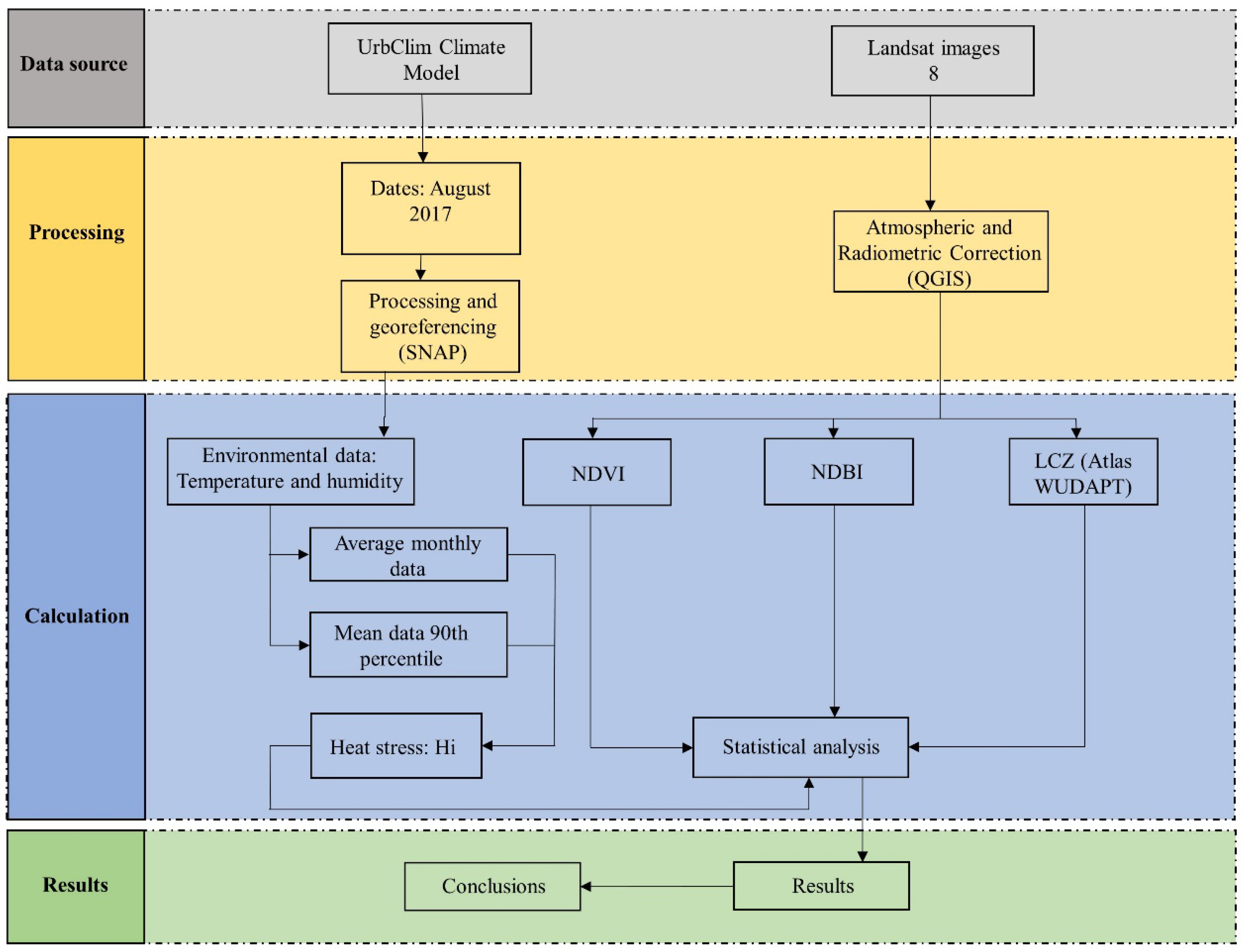
The methodology carried out for this research can be seen in Figure 2. Using Landsat 8 images, NDVI and NDBI indices were obtained at a resolution of 15 m. Next, the high-precision plane of the different LCZs of the WUDAPT atlas was downloaded. This database is supported by the values of observation and numerical modelling for the different thermal characteristics of cities [14,27]. Its use in soil identification studies using LCZ is widely documented [14,28,29]. The average values of relative humidity and ambient temperature for the month of August 2017 were obtained from the UrbClim model of the European Space Agency (ESA). The calculation of Hi was made with average temperatures and with temperatures exceeding the 90th percentile. With these data, the heat stress index in the different LCZ was determined and subsequently correlated with the rest of the indices through the help of statistical analysis using the STATA software, version 16. The ANOVA analysis and the data panel were used to determine and analyze the significant correlations of the variables.

2.3. Landsat 8 Imagery

The Landsat 8 imagery was obtained from the United States Geological Survey (USGS, Reston, VA, USA) for the month of August 2017. The Landsat satellite has ten bands with a resolution ranging from 100 to 15 m. However, a band resampling process was applied to the images with the help of the Sentinel Applications Platforms (SNAP, Brockmann Consult, Hamburg, Germany; Array Systems, Los Angeles, CA, USA) software using the bicubic methodology due to the high quality of the results obtained. It was taken into account that the cloudiness of the selected days was not more than 5% in order to increase the uptake of urban areas. After downloading, the images underwent an atmospheric correction process in OLI bands. For this reason, the process described by the authors [30,31] was followed using the dark object subtraction (DOS) algorithm with the help of the QGIS software, (OSGeo, Beaverton, OR, USA) [8,32]. NDVI is calculated using spectral bands according the Equation (1). With NDBI, we can determine the proportion of built-up areas compared to areas without buildings using the Equation (2) [33]:

$$NDVI=\frac{NIR-Red}{NIR+Red}$$

(1)

$$NDBI=\frac{SWIR-NIR}{SWIR+NIR}$$

(2)

2.4. LCZ Mapping

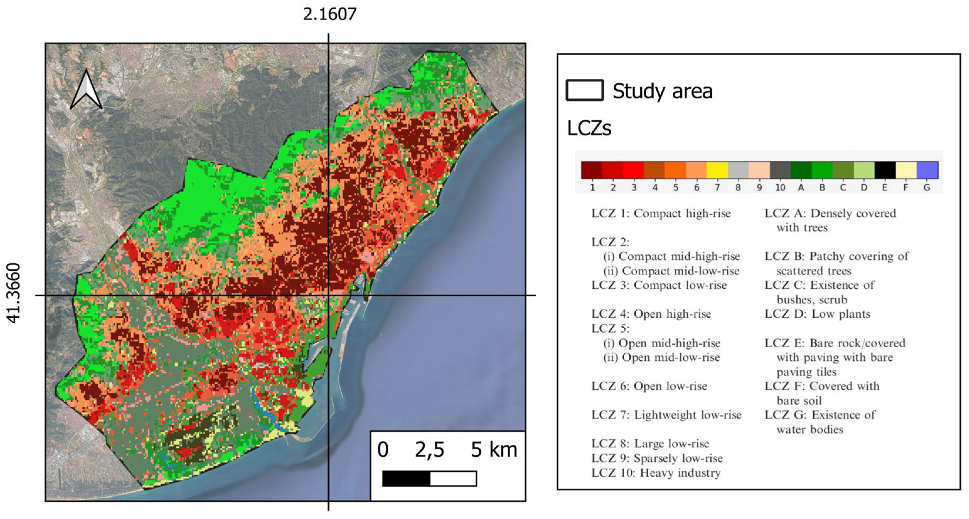
The LCZ map of the city of Barcelona (Figure 3) can be found within the WUDAPT atlas database [14,27] (https://LCZ-generator.rub.de/submissions (accessed on 25 September 2023)), which is based on the classification established by Steward and Oke [24].

The identification of the different LCZ allows cataloguing areas that have a specific thermal regime over time based on their situation and morphological characteristics [5]. Its use in landscape characterization studies is widely documented [28,29,34,35]. Figure 4 shows the surface area (%) occupied by each LCZ within the city of Barcelona. In this way, it can be observed how the LCZ with greater extension are 2, 5, D, and A, while those with less extension are LCZ G, 8, E, and 6.

The accuracy value reported by the WUDAPT atlas for the city is 0.69. However, a comparison of the different LCZs was made with Landsat and Google Street View satellite imagery. In general, the LCZs of the atlas are consistent with satellite images and Google Street View, presenting values that fall within the patterns defined by the authors Stewart and Oke [36].

2.5. Urbclim Model and Study Period

The environmental temperature and relative humidity data of the city on the established dates were obtained from the UrbClim model developed by ESA’s Copernicus programmed. This is based on a transfer scheme between the Land Surface Atmosphere and the geosphere called Land Surface Interaction Calculation (LAICA) that was later modified to include the surfaces of urban areas [16]. The use of the UrbClim model was validated through studies carried out in several European cities such as Madrid [17], Antwerp, Bruges, and Ghent [14].

In order to know the different periods under study, the temperature data of the AEMET were taken into account. Thus, in 2017, the month with the highest temperatures in the city of Barcelona was August. This month’s employment is motivated by the fact that it was the hottest month of the 2000–2017 series in the city. Within this month, temperatures had average values on days 10, 11, and 31 and exceeded the 90th percentile on days 2, 3, 4, 5, 17, 18, 23, 24, 25, 28, and 29. Therefore, data from these days were obtained for the study in a period of average temperatures and above the 90th percentile.

2.6. Heat Stress Index (Hi)

To obtain the heat stress index, the Hi formula developed in 1990 [36] and subsequently modified [37] according to Formula (3) was used:

$$\begin{array}{ll}\mathrm{H}\mathrm{e}\mathrm{a}\mathrm{t} \mathrm{I}\mathrm{n}\mathrm{d}\mathrm{e}\mathrm{x}\left(\mathrm{H}\mathrm{i}\right)& =-8.78469475556+(1.61139411\times T)+(2.33854883889\times H)\\ & -(0.14611605\times T\times H)-(0.012308094\times T^2)-(0.0164248277778\times H^2)\\ & +(0.002211732\times T^2\times H)+(0.00072546\times T\times H^2)-(0.000003582\times T^2\times H^2)\end{array}$$

(3)

where Hi is the heat stress index in °C, T is the air temperature in °C, and H is the relative humidity in %. Based on the results obtained, the effects on the population can be known based on

Table 1. Classification of heat indices and heat risk conditions.

Heat Index	Classification of Heat	Hi (°C)	General Effect on People
Hi-1	No Risk	<26.00	No risk to population group.
Hi-2	Very Warm	26.66–32.21	Fatigue possible with prolonged exposure and physical activity.
Hi-3	Hot	32.22–39.43	Sunstroke, heat cramps, or heat exhaustion LIKELY and heat stroke POSSIBLE with prolonged exposure and/or physical activity.
Hi-4	Very Hot	39.44–51.10	Sunstroke, heat cramps, or heat exhaustion POSSIBLE with prolonged exposure and/or physical activity.
Hi-5	Extremely Hot	>51.11	Heat/sunstroke HIGHLY LIKELY with continued exposure.

Source: [13].

[13].

3. Results

3.1. NDVI and NDBI Indices

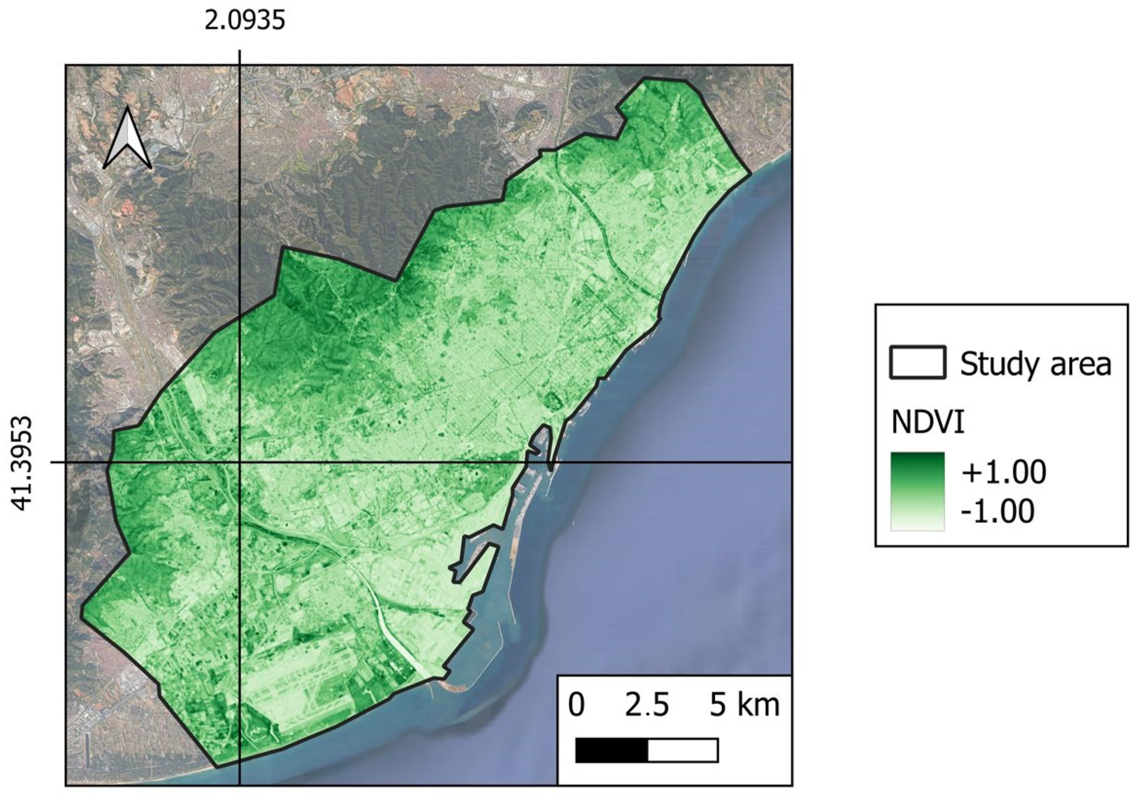
The examination of the NDVI and NDBI indices for the city of Barcelona during the month of August 2017 is depicted in Figure 5 and Figure 6. The computed average values for these indices across the city are as follows: NDVI (0.155) and NDBI (0.198). The NDVI value of 0.155 implies that the vegetation within the city can be characterized as consistent and suitable for the month of August. On the other hand, the NDBI value of 0.198 suggests that the urban landscape predominantly consists of compact areas with medium to high population density, contrasting with open areas featuring lower density.

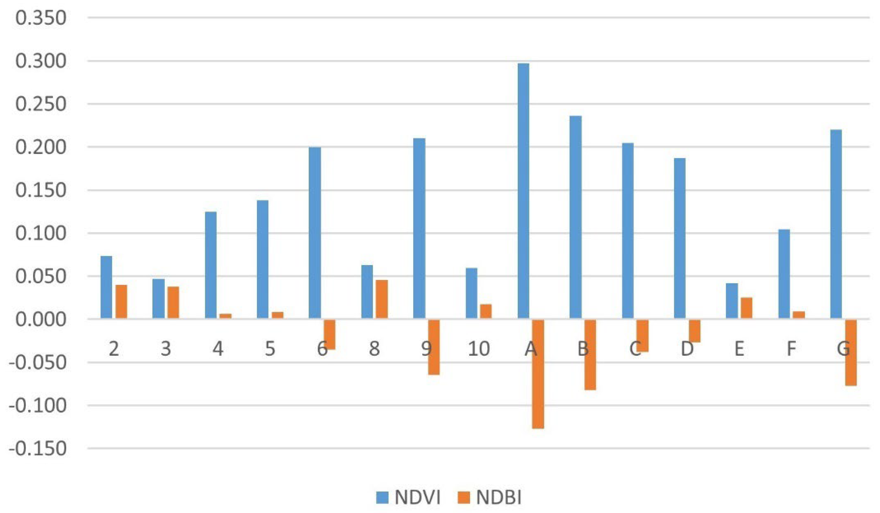
Figure 7 displays the average NDVI and NDBI values for each land cover zone (LCZ) within the city of Barcelona. The NDVI index demonstrates the highest values in rural zones, specifically LCZ-A (0.297), B (0.236), G (0.223), 9 (0.211), and C (0.205), while the lowest values are observed in urban, industrial, and compact areas, particularly LCZ-E (0.042), 3 (0.047), 8 (0.063), 10 (0.069), and 2 (0.073). Moreover, when considering urban areas exclusively, compact LCZs exhibit lower NDVI values (0.060) compared to open areas (0.131). These findings regarding vegetation highlight a denser presence of leafy greenery in rural and open areas, contrasting with the comparatively lower vegetation cover in industrial and compact urban zones within the city.

The most elevated NDBI values are observed in urban zones: LCZ-8 (0.1045), LCZ-2 (0.040), LCZ-3 (0.038), and LCZ-10 (0.018). Conversely, the lowest values are found in rural regions: LCZ-A (−0.127), LCZ-B (−0.082), LCZ-G (−0.077), and LCZ-9 (−0.064). Additionally, when considering urban areas exclusively, compact LCZs exhibit higher NDBI values (0.039) in contrast to open areas (0.008). These values indicate that urban regions have a more extensive and denser building presence compared to rural areas. Furthermore, within urban settings, compact and industrial areas tend to have a higher degree of building occupation than open areas.

Table 2. ANOVA test results for NDVI and NDBI indices.

	NDVI	NDBI
Difference of Square	0.0001 ***	0.0001 ***
R2	302.228	248.033

Robust standard errors: *** p < 0.001. R², linear regression coefficient.

shows the results of the statistical analysis–ANOVA for the indices (NDVI and NDBI). Both present distributions of values classified as non-normal within each LCZ but have statistically significant relationships greater than 99%.

3.2. Spatiotemporal Evaluation of Temperature

In Figure A1 and Figure A2 of the Appendix A, one can see the spatiotemporal analysis of the average ambient temperature per hour of the city of Barcelona with the average values and with the values above the 90th percentile. It is reported that the lowest temperatures in both environmental situations are located in rural areas or outside urban areas. These areas have higher values of the NDVI index and lower values of the NDBI index. On the contrary, the highest temperatures are located in urban areas. The average temperature of the city of Barcelona with normal values was 26.87 °C, while the average temperature when the values were above the 90th percentile was 30.07 °C, which reports an average increase of 11.90%. These values correspond to the weighted average of each value in the corresponding pixel.

It can be observed (Figure 8) how the average increases in temperatures were higher in the urban LCZ (2, 3, 4, 5, 6, 8, 9, and 10) with an average value of 11.06% compared to the rural LCZ (A, B, C, D, E, F, and G) where the average growth was 10.59%. It can also be seen how within the urban LCZ the growth was higher in the compact LCZ (2 and 3) (11.02%) compared to the open areas (4, 5, and 6) where the growth was 10.57%. This circumstance could be motivated by two important factors: the use of impermeable materials with high thermal absorption in the construction of urban areas and the low rates of surfaces destined to green areas that prevent the cooling of cities. Building materials such as asphalt, bricks, and concrete heat up during the day due to the solar radiation they receive, and after the sun sets, they release the heat absorbed during the day into the atmosphere. This sudden warming is what produces and intensifies the urban heat island (UHI) phenomenon [6,11,38]. On the other hand, the regular distribution of trees in streets and green areas in cities has been considered one of the most effective strategies to avoid environmental warming [39].

Table 3. ANOVA test results for temperatures.

Sources	Temperature
Difference of Square	0.0001 ***
R2	294.835

Robust standard errors: *** p < 0.001. R², linear regression coefficient.

shows the results of the temperature by LCZs. Both present distributions of values classified as non-normal within each LCZ but have statistically significant relationships greater than 99%.

To establish the relationships between temperature and the various indices (NDVI and NDBI), a statistical analysis technique known as the data panel was employed. Initially, the Pearson correlation coefficient was computed, and subsequent analysis was conducted. The results are presented in

Table 4. Pearson’s coefficient between temperature and NDVI and NDBI indices.

	Temperature	NDVI	NDBI
Temperatures	1
NDVI	−0.676	1
NDBI	0.593	−0.877	1

and

Table 5. Results between temperature and NDVI and NDBI indices.

	β	p	sd
NDVI	−9.461	0.000 ***	0.9623
NDBI	0.028	0.000 ***	1.2810
	R2 = 0.46	F = 209.52	Prob > chi2 = 0.00

β, coefficient. Robust standard errors: *** p < 0.001. sd, standard deviation; R², linear regression coefficient; F, statistical.

.

Table 4 indicates that temperature exhibits a positive correlation with the NDBI index (0.593) and a negative correlation with the NDVI index (−0.676). These findings suggest that as temperature increases, there is a tendency for higher values of the NDBI index, signifying greater urban density. Conversely, higher temperatures are associated with lower NDVI values, indicating reduced vegetation density.

The statistical analysis yielded significant and robust results, confirming the relationships identified earlier. Specifically, the results indicate a statistically significant and positive relationship above the 99% confidence level between the ambient temperature variable and the NDBI variable. In contrast, there is a negative relationship above the 99% confidence level with the NDVI variable. The statistical model’s goodness of fit is exceptionally high, with a significance level exceeding 99%, as evidenced by the Prob > Chi² value of 0.000. These analytical findings provide strong empirical support for the previously established relationships.

3.3. Spatiotemporal Evaluation of Humidity

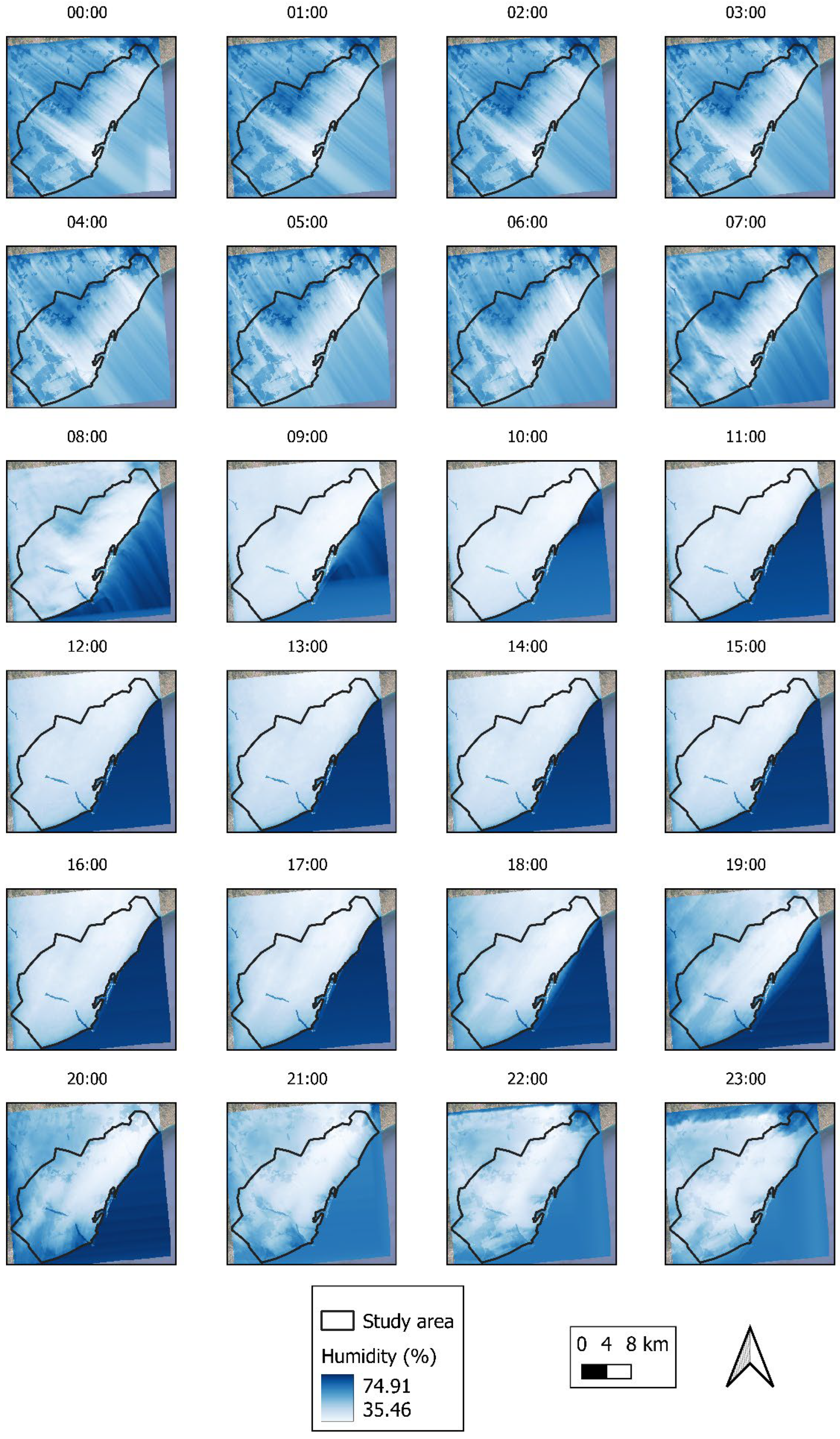
Figure A3 and Figure A4 of Appendix A show the spatiotemporal analysis of the average hourly humidity of the city of Barcelona in the two environmental situations studied. It is observed that the highest humidity values in both situations are concentrated in rural areas (higher values of the NDVI indices), while the lowest values are located in urban areas (higher values of the NDBI indices). The average humidity of the city of Barcelona under normal environmental conditions was 64.87%, while the average humidity when the temperature values were above the 90th percentile was 53.17%. These values demonstrate a decrease of 17.78%.

The analysis reveals noteworthy patterns in humidity distribution across different land cover zones (LCZs) in the study area (Figure 9). Specifically, humidity levels are notably higher in rural LCZs (A, B, C, D, E, F, and G) compared to urban LCZs (2, 3, 4, 5, 6, and 8). Additionally, it is evident that the reduction in humidity when the temperature rises is less pronounced in rural LCZs (−15.62%) as opposed to urban LCZs (−18.69%). This variation can be attributed to the phenomenon of evapotranspiration from plant elements. During periods of elevated temperatures, these elements release moisture into the atmosphere, contributing to an environmental cooling effect [40]. Moreover, within urban areas, compact LCZs (2 and 3) exhibit relatively smaller declines in humidity (−19.05%) compared to open LCZs (4, 5, and 6) (−19.43%). This difference may be attributed to the fact that open areas have higher values in the NDVI indices, indicating more extensive green spaces with vegetation. These green areas enhance ambient humidity through the process of evapotranspiration, mitigating the decrease in humidity during temperature spikes.

Table 6. ANOVA test results for humidity.

Sources	Humidity
Difference of Square	0.0001 ***
R2	295.147

Robust standard errors: *** p < 0.001. R², linear regression coefficient.

shows the results of the humidity by LCZs. Both present distributions of values classified as non-normal within each LCZ but have statistically significant relationships greater than 99%.

3.4. Heat Stress Index (Hi)

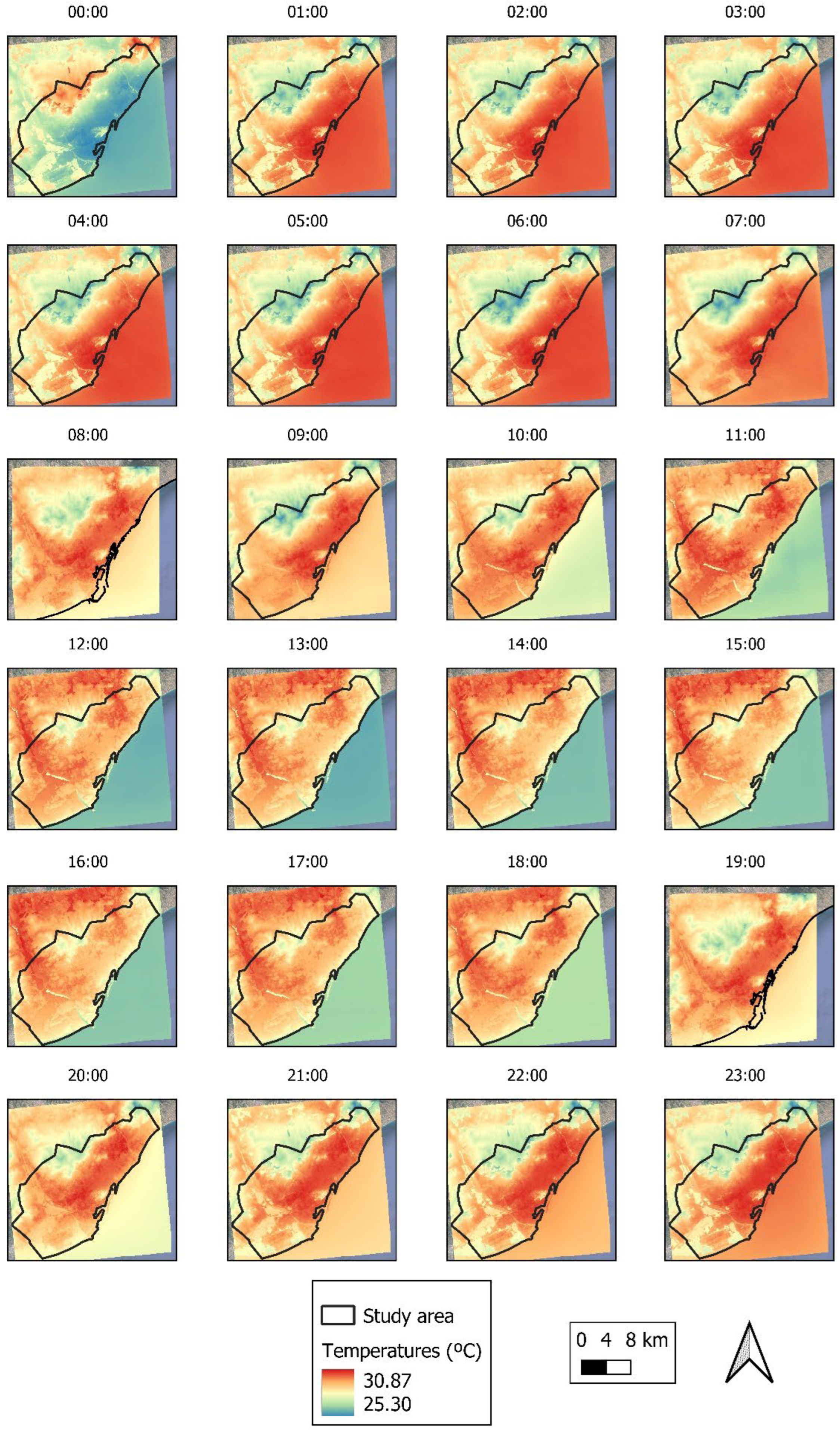
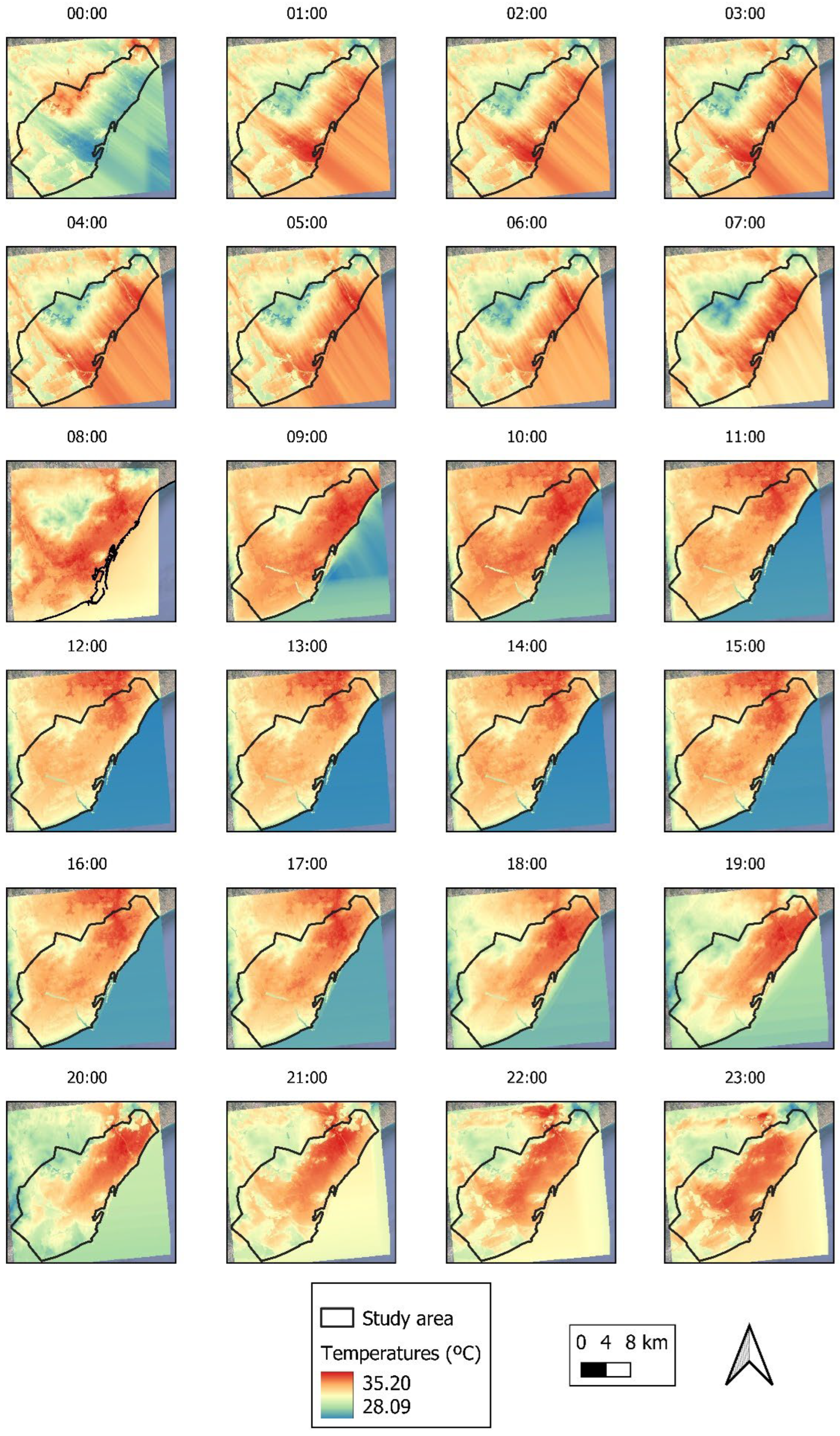
In Figure A5 and Figure A6 of Appendix A, one can see the spatial temporal analysis of the average Hi by hours of the city of Barcelona in the two environmental situations investigated. It can be seen how the lowest values of Hi in both situations are concentrated in areas outside urban or rural areas (lower values of the NDBI indices), while the highest values are located in urban areas and within them in the city center (lower values of the NDVI indices). During the days with average temperature values, the Hi was 26.87 °C, while the days with temperatures above the 90th percentile take a value of 31.22 °C. This represents an average increase of 16.19%.

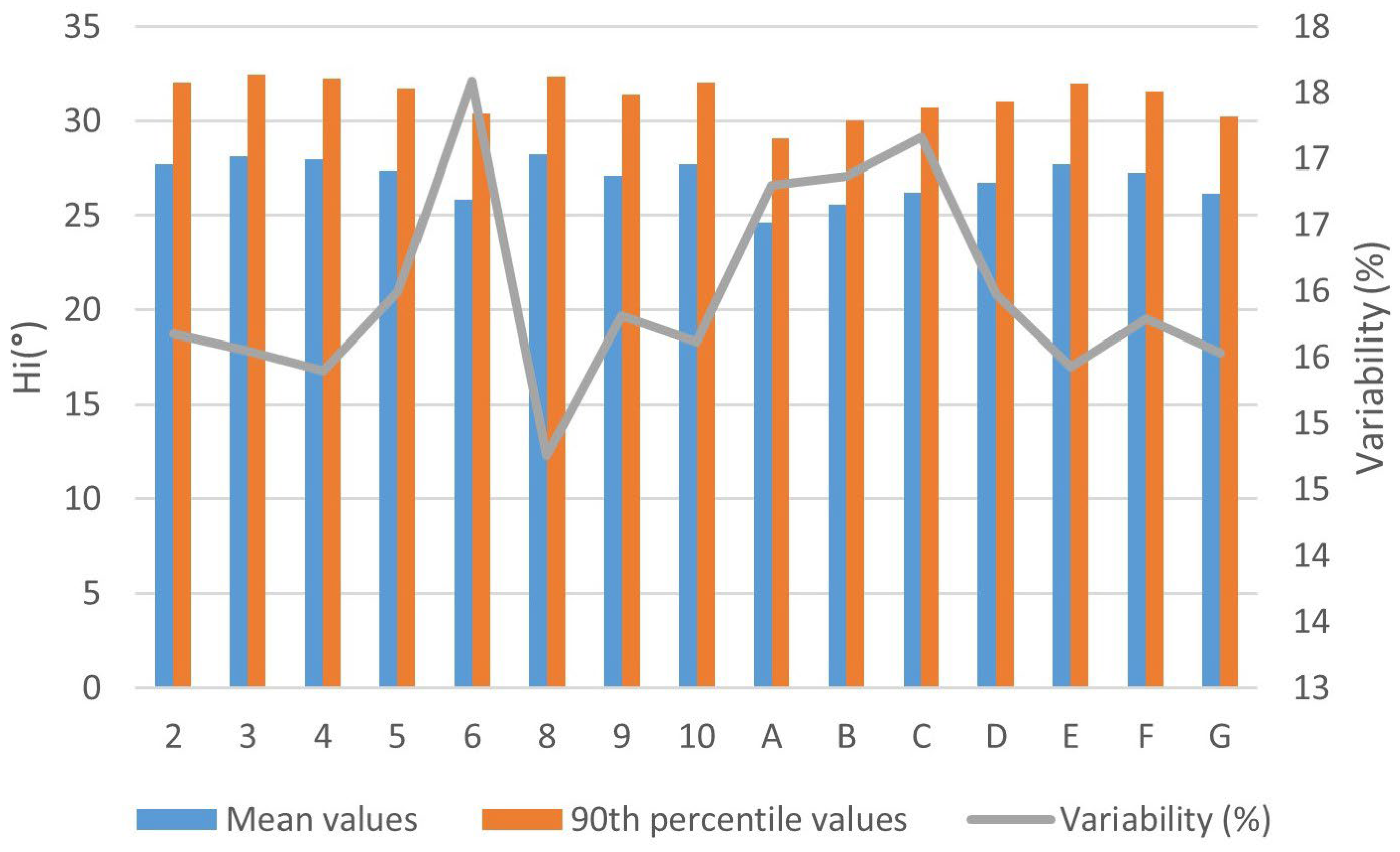
The analysis reveals that the highest Hi values (Figure 10), in both situations considered, are concentrated in urban areas (characterized by higher NDBI values), whereas the lowest Hi values are situated in rural areas or on the outskirts of the city (associated with higher NDVI values). Furthermore, it is evident that the most substantial increases in Hi occur in urban land cover zones (LCZs 2, 3, 4, 5, 6, 8, 9, and 10), while, conversely, the increases are more modest in rural LCZs (A, B, C, D, E, F, and G). In specific terms, the city of Barcelona has witnessed an average Hi growth of 15.80% in urban LCZs, whereas the growth in rural LCZs has been slightly lower at 14.20%. This demonstrates that the urban areas have experienced a relatively higher increase in heat stress compared to the rural areas, reflecting the impact of urbanization and its associated factors on thermal stress levels.

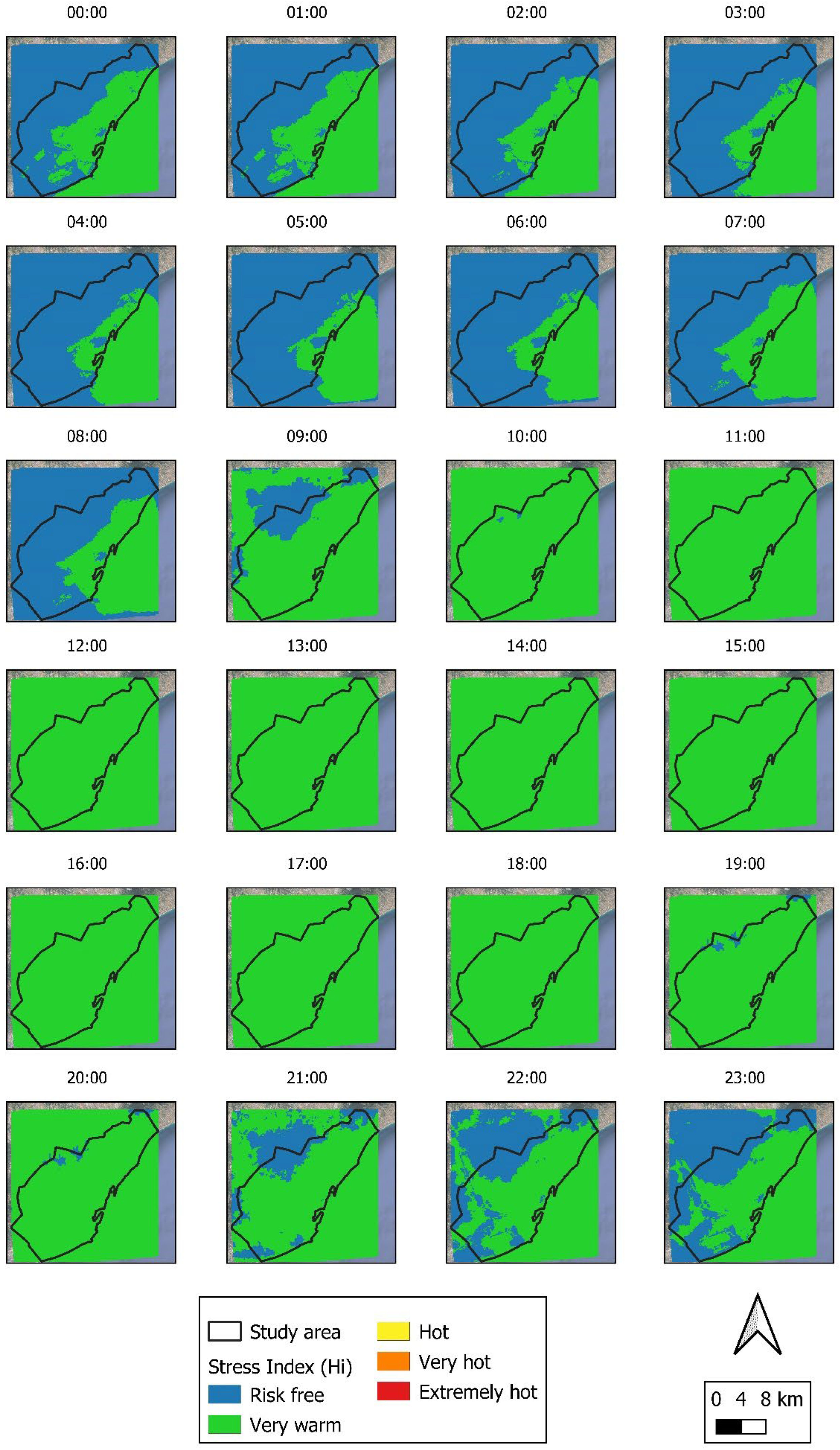
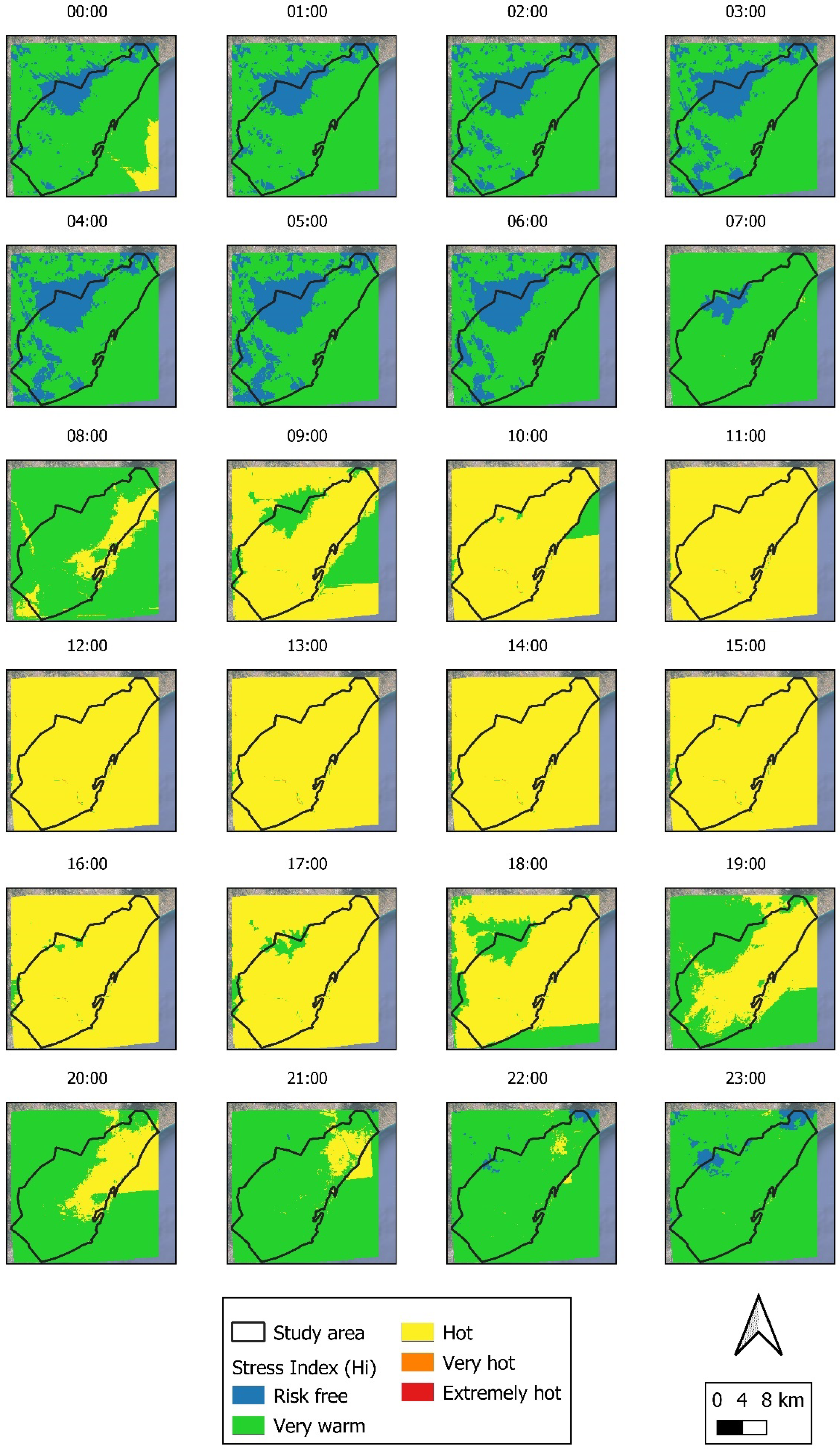
Figure A7 and Figure A8 of Appendix A show the rating of the Hi index as a function of the effects on the population (Table 1) under normal environmental conditions and when the values were above the 90th percentile. It can be observed how in normal environmental conditions and during daytime hours, the city of Barcelona presents an index rated as very warm that is minimized to the rating of without risk during the night hours. In conditions above the 90th percentile, there is a strengthening of the Hi stress index in such a way that during the night hours, the areas classified without risk are transformed to very warm areas, and during the daytime hours, the areas classified as very warm become classified as hot.

Figure 11 shows the result of Hi under both environmental conditions for each LCZ. In a situation of average temperatures, the open zones (3 and 4) and zones without coverage (E) heat up quickly before the reception of the first rays of sun. On the contrary, and when it gets dark, rural areas cool quickly compared to urban areas that maintain high temperatures until dawn. In a situation of temperatures above the 90th percentile, all LCZs warm up quickly, but open and rural LCZs cool more quickly once the sun goes down.

Table 7. ANOVA test results for Hi.

Sources	Hi
Difference of Square	0.0001 ***
R2	294.835

Robust standard errors: *** p < 0.001. R², linear regression coefficient.

displays the Hi results categorized by LCZs. In both cases, the distributions of values within each LCZ are characterized as non-normal. However, there are statistically significant relationships exceeding 99% between different LCZs, both during normal environmental conditions and heatwave periods.

Table 8. Pearson’s coefficient between Hi and NDVI, NDBI, and LCZ indices at normal temperatures.

	Hi	NDVI	NDBI	LCZ
Hi	1
NDVI	−0.675	1
NDBI	0.592	−0.877	1
LCZ	−0.471	0.422	−0.414	1

and

Table 9. Data Panel results between Hi and NDVI, NDBI, and LCZ indices at normal temperatures.

	β	p	sd
NDVI	−8.643	0.000 ***	0.9623
NDBI	0.842	0.000 ***	1.2810
LCZ	−0.063	0.000 ***	0.0097
	R2 = 0.49	F = 163.78	Prob > chi2 = 0.00

β, coefficient. Robust standard errors: *** p < 0.001. sd, standard deviation; R², linear regression coefficient; F, statistical.

present the outcomes of the statistical analysis. Table 8 highlights the positive correlation between Hi and the NDBI index (0.592), signifying that higher building density, as indicated by NDBI, corresponds to elevated Hi values. Conversely, Hi exhibits a negative correlation with the NDVI (−0.655) and LCZ (−0.471) indices. This indicates that regions with more abundant vegetation cover (reflected in NDVI) and areas categorized as non-urban (LCZ) tend to have lower Hi values, underscoring the cooling effect of vegetation and the mitigating impact of non-urban land cover on heat stress.

The results report a positive relationship of more than 99% with the NDBI variable and a negative relationship with the NDVI and LCZ variables.

The process of statistical analysis is repeated in the periods of heat wave suffered in the city of Barcelona.

Table 10. Pearson’s coefficient between Hi and NDVI, NDBI, and LCZ indices with warm temperatures.

	Hi	NDVI	NDBI	LCZ
Hi	1
NDVI	−0.693	1
NDBI	0.610	−0.867	1
LCZ	−0.481	0.411	−0.403	1

shows how the Hi again presents a positive correlation with the NDBI index (0.610) and a negative correlation with the NDVI (−0.693) and LCZ (−0.481) indices. The variables investigated have a higher correlation in conditions of temperatures above the 90th percentile than in average temperatures. Therefore, the relationships between the variables are stronger when temperatures increase.

Table 11. Data panel results between Hi and NDVI, NDBI, and LCZ indices with warm temperatures.

	β	p	sd
NDVI	−8.422	0.000 ***	0.929
NDBI	0.962	0.000 ***	1.221
LCZ	−0.066	0.000 ***	0.010
	R2 = 0.22	F = 10.15	Prob > chi2 = 0.00

β, coefficient. Robust standard errors: *** p < 0.001. sd, standard deviation; R², linear regression coefficient; F, statistical.

shows the results of the statistical analysis in ambient conditions above the 90th percentile repeat the previous results.

4. Discussion

The analysis of the NDVI and NDBI indices in relation to land cover and urban morphology reveals distinct patterns within the study area. Firstly, it is evident that the NDVI index, which is associated with vegetation, exhibits higher values in rural areas (LCZ-A, B, C, D, E, F, and G) and open urban areas (LCZ-4, 5, and 6). Conversely, industrial and compact urban areas (LCZ-2, 3, and 10) display lower NDVI values. This indicates that rural and open urban areas have more extensive vegetation cover, while industrial and compact urban zones have less greenery. On the other hand, the NDBI index, linked to building density, showcases higher values in urban areas (LCZ-2, 3, 5, 6, and 10) compared to rural areas (LCZ-A, B, C, D, E, F, and G), where NDBI values are lower. Moreover, among urban LCZs, the NDBI values are higher in compact zones (2 and 3) as opposed to open areas (4, 5, 6, 8, and 9), where NDBI values are lower. This trend highlights the correlation between building density and NDBI values. In areas with higher building density, NDBI values are elevated, while in areas with lower building density, NDBI values are lower. These observations collectively define the urban morphology of each city and LCZ under investigation, reflecting the extent of vegetation and building density within these regions. These results are in line with other studies conducted by other authors [6,41,42,43,44,45] in other cities and territories allowing to validate the data obtained in this research. These studies report results that mainly relate low NDVI values with high NDBI index values in compact areas of cities. Conversely, high NDVI values are related to low NDBI values in rural areas.

The analysis revealed a significant increase in temperatures during warm periods. Interestingly, when examining both periods under investigation, it becomes apparent that urban areas tend to have lower temperatures during the morning hours compared to rural areas. However, as the day progresses, urban temperatures surpass those in rural areas. Several factors contribute to this pattern. Firstly, during the morning hours, urban areas receive less solar radiation compared to rural areas. This can be attributed to several factors. First, the presence of trees and buildings in urban areas casts shadows, reducing the amount of direct sunlight reaching the ground. Second, urban areas often consist of heterogeneous surfaces with high thermal absorption properties. These surfaces contribute to lower morning temperatures, as they absorb less heat from the sun. Lastly, the presence of vegetation in urban areas has a cooling effect on the environment during the morning, while areas lacking greenery experience warming rates. The shadows created by trees and buildings in cities, particularly in compact urban areas, play a pivotal role in preventing the rapid heating of surfaces when solar radiation is limited during the morning hours. This phenomenon contributes to the observed temperature variations between urban and rural areas throughout the day. This prevents these heated walls from subsequently releasing high doses of heat into the atmosphere and altering the temperature of the area [43,46,47]. On the contrary, the temperature during the night hours is higher in urban areas as opposed to rural areas, where it is lower. This is motivated by the fact that once the sun goes down, urban areas tend to cool slowly since heat is conserved, while rural areas cool quickly. The more compact an area is, the more surface area of walls it has, and the more heat is retained in them. The use of waterproof construction materials with high thermal absorption inside cities causes them, after the sun goes down, to release the heat absorbed during the day [39,43,48]. Within urban areas, the temperature is higher in compact and industrial areas (LCZ-2, 3, and 10) than in open areas (LCZ-4, 5, and 6). This circumstance is again influenced in the configuration presented by the LCZ-4, 5, and 6, with buildings located at great distances and large green spaces with vegetation. Numerous studies have shown that vegetation has a cooling effect in urban areas [49,50,51], ranging from 1 to 3 °C. Our results are in line with the results reported by other authors [14,15,17] who used the UrbClim climate model in their studies of other European cities.

The analysis underscores a significant decrease in humidity levels during periods of elevated temperatures. However, consistently across both periods studied, humidity values are higher in rural areas when compared to urban areas, where humidity levels are notably lower. Specifically, the lowest humidity values are observed in compact and industrial areas (LCZ 2, 3, 10, and 6). As previously noted, these areas exhibit lower NDVI and PV indices and higher values in the NDBI and UI indices. Concurrently, they also experience higher temperatures. This observed correlation can be attributed to the presence of vegetation and its evapotranspiration process. The amount of vegetation surface directly influences the magnitude of evapotranspiration. In areas with more extensive plant cover, the evapotranspiration process is more pronounced. Consequently, this leads to higher ambient humidity levels and lower temperatures. In summary, the amount of vegetation available within the different LCZs plays a crucial role in influencing humidity levels and, consequently, temperature variations within these areas. This circumstance is corroborated by the study carried out on four cities in the Tennessee region (TN, USA), where it was reported that trees minimize the heat effect due to increased environmental humidity [19]. This circumstance denotes that our results are in line with the research carried out by other authors [14,15,17] who used the UrbClim climate model in their studies of other European cities.

An important variability of Hi was evidenced in the different LCZs of the city both with average temperatures and with temperatures above the 90th percentile. Thus, and during the first periods, heat stress during the day can be qualified as very warm between 12:00 and 19:00 h in all LCZs. On the contrary, and during the nights and at dawn (22:00 and 09:00 h), the heat stress index can be qualified as without risk. It has been corroborated how rural LCZs with vegetation increase in Hi more slowly during the morning hours (10:00 and 11:00 h), while in the afternoons, it is reduced more quickly there than in urban areas. During periods of ambient temperatures above the 90th percentile, a significant intensification of Hi is reported in the different LCZ, especially between 9:00 and 19:00 h, where a hot Hi is reported. In the mornings, Hi intensifies rapidly in all LCZs, but in the afternoons, it decreases in intensity more rapidly in rural areas. In this sense, compact and industrial LCZs (LCZ-2, 3, and 10) have higher Hi values and maintain intensity for longer than open areas (LCZ-4, 5, and 6) that minimize the value in less time. This is because the built-up areas of the city have a higher percentage of impermeable materials that absorb heat more quickly compared to rural areas. At night, this heat is released into the atmosphere, maintaining high values of Hi and needing more time to minimize its effects. This trend was observed and reported in studies on the cities of Kolkata, Chenai, Delhi, Mumbai, and Nagpur (India), where the studies related the areas with the largest built-up area and less vegetation cover with the hottest areas and with higher Hi [13,21]. In turn, our results are in line with the research carried out by other authors [14,15,17]. The regression model reported statistically significant and negative relationships between Hi and NDVI and LCZ indices and positive relationships with the NDBI variable, evidencing what was reported analytically. In turn, these relationships intensify under conditions of temperature increases, signifying the importance of green areas as a measure to mitigate the effects of Hi on the population. Therefore, our results report a greater and faster growth of the HI index and a subsequent slower decrease compared to studies that used average temperatures [14,15,16].

5. Conclusions

This study assessed the heat stress index (Hi) in Barcelona during August 2017, utilizing data from ESA’s UrbClim climate model both under conditions of average temperatures and during periods when temperatures exceeded the 90th percentile. To enhance the evaluation and facilitate the extrapolation of results to other cities, the well-established classification of land areas based on land cover zones (LCZ) was employed.

The findings indicate that a significant portion of Barcelona’s population experienced an average heat stress index classified as “very warm” during the daytime and “without risk” during the nights in the presence of average temperatures. However, these values increased notably on days when temperatures exceeded the 90th percentile, categorizing the daytime Hi as “hot” and the nights as “very warm”.

Furthermore, the analysis revealed substantial temporal and spatial variability in Hi, with considerable increases during intense heat episodes. A positive correlation was established between Hi and the NDBI index, while a negative correlation was observed with the NDVI and LCZ indices. Hi values were notably higher in compact and industrial LCZs (LCZ-2, 3, and 10) compared to open and rural LCZs (LCZ-4, 5, 6, D, B, and G), which exhibited lower Hi values and greater resilience to extreme heat events. This underscores that areas with higher percentages of impervious surfaces and fewer green spaces are more susceptible to experiencing higher levels of heat stress. Moreover, these areas tend to heat up faster and retain heat for longer periods.

Based on these results, it is recommended that urban planning for new areas prioritize open spaces with substantial green areas over compact, high-density developments with limited green spaces. Additionally, to increase greenery in existing compact areas, the use of green facades and green roofs is proposed. Such measures can significantly enhance the resilience of urban areas to extreme heat events, ultimately improving the quality of life for city residents.

Regarding the limitations of this study, it is necessary to review the need to obtain more updated data regarding humidity and temperature values. Remember that the last five summers have been classified by ESA’s Copernicus as the five warmest of the centuries. Therefore, and as future lines of research, it is necessary to update the data presented here with the values of recent summers in order to improve the predictions presented here and improve people’s quality of life.

References

1. Mora, C.; Dousset, B.; Caldwell, I.R.; Powell, F.E.; Geronimo, R.C.; Bielecki, C.R.; Counsell, C.W.W.; Dietrich, B.S.; Johnston, E.T.; Louis, L.V.; et al. Global risk of deadly heat. Nat. Clim. Change 2017, 7, 501–506. [Google Scholar] [CrossRef]
2. IPCC. The Fifth Report of the Intergovernmental Panel on Climate Change (IPCC). 2013. Available online: https://www.ipcc.ch/report/ar5/wg1/ (accessed on 25 September 2023).
3. Li, J.; Song, C.; Cao, L.; Zhu, F.; Meng, X.; Wu, J. Impacts of landscape structure on surface urban heat islands: A case study of Shanghai, China. Remote Sens. Environ. 2011, 115, 3249–3263. [Google Scholar] [CrossRef]
4. Song, J.; Chen, W.; Zhang, J.; Huang, K.; Hou, B.; Prishchepov, A.V. Effects of building density on land surface temperature in China: Spatial patterns and determinants. Landsc. Urban Plan. 2020, 198, 103794. [Google Scholar] [CrossRef]
5. Stewart, I.D.; Oke, T.R. Local climate zones for urban temperature studies. Bull. Am. Meteorol. Soc. 2012, 93, 1879–1900. [Google Scholar] [CrossRef]
6. Hidalgo García, D.; Arco Díaz, J. Modeling of the Urban Heat Island on local climatic zones of a city using Sentinel 3 images: Urban determining factors. Urban Clim. 2021, 37, 100840. [Google Scholar] [CrossRef]
7. Hua, L.; Zhang, X.; Nie, Q.; Sun, F.; Tang, L. The impacts of the expansion of urban impervious surfaces on urban heat islands in a coastal city in China. Sustainability 2020, 12, 475. [Google Scholar] [CrossRef]
8. García, D.H.; Díaz, J.A. Space–time analysis of the earth’s surface temperature, surface urban heat island and urban hotspot: Relationships with variation of the thermal field in Andalusia (Spain). Urban Ecosyst. 2023, 26, 525–546. [Google Scholar] [CrossRef]
9. UNO. 68% of the World Population Projected to Live in Urban Areas by 2050, Says UN. 2018. Available online: https://www.un.org/development/desa/en/news/population/2018-revision-of-world-urbanization-prospects.html (accessed on 25 September 2023).
10. Schneider, A.; Friedl, M.A.; Potere, D. Mapping global urban areas using MODIS 500-m data: New methods and datasets based on “urban ecoregions”. Remote Sens. Environ. 2010, 114, 1733–1746. [Google Scholar] [CrossRef]
11. Santamouris, M. Recent progress on urban overheating and heat island research. Integrated assessment of the energy, environmental, vulnerability and health impact. Synergies with the global climate change. Energy Build. 2020, 207, 109482. [Google Scholar] [CrossRef]
12. Jacobs, C.; Singh, T.; Gorti, G.; Iftikhar, U.; Saeed, S.; Syed, A.; Abbas, F.; Ahmad, B.; Bhadwal, S.; Siderius, C. Patterns of outdoor exposure to heat in three South Asian cities. Sci. Total Environ. 2019, 674, 264–278. [Google Scholar] [CrossRef]
13. Kotharkar, R.; Ghosh, A.; Kotharkar, V. Estimating summertime heat stress in a tropical Indian city using Local Climate Zone (LCZ) framework. Urban Clim. 2021, 36, 100784. [Google Scholar] [CrossRef]
14. Verdonck, M.L.; Demuzere, M.; Hooyberghs, H.; Beck, C.; Cyrys, J.; Schneider, A.; Dewulf, R.; Van Coillie, F. The potential of local climate zones maps as a heat stress assessment tool, supported by simulated air temperature data. Landsc. Urban Plan. 2018, 178, 183–197. [Google Scholar] [CrossRef]
15. Geletič, J.; Lehnert, M.; Savić, S.; Milošević, D. Modelled spatiotemporal variability of outdoor thermal comfort in local climate zones of the city of Brno, Czech Republic. Sci. Total Environ. 2018, 624, 385–395. [Google Scholar] [CrossRef] [PubMed]
16. De Ridder, K.; Lauwaet, D.; Maiheu, B. UrbClim—A fast urban boundary layer climate model. Urban Clim. 2015, 12, 21–48. [Google Scholar] [CrossRef]
17. Martí Ezpeleta, A.; Royé, D. Intensidad y duración del estrés térmico en verano en el área urbana de Madrid. Geographicalia 2021, 73, 95–113. [Google Scholar] [CrossRef]
18. Royé, D.; Sera, F.; Tobías, A.; Lowe, R.; Gasparrini, A.; Pascal, M.; De’Donato, F.; Nunes, B.; Teixeira, J.P. Effects of Hot Nights on Mortality in Southern Europe. Epidemiology 2021, 32, 487–498. [Google Scholar] [CrossRef]
19. Hass, A.L.; Ellis, K.N.; Mason, L.R.; Hathaway, J.M.; Howe, D.A. Heat and humidity in the city: Neighborhood heat index variability in a mid-sized city in the Southeastern United States. Int. J. Environ. Res. Public Health 2016, 13, 117. [Google Scholar] [CrossRef]
20. Pani, S.K.; Lin, N.H.; RavindraBabu, S. Association of COVID-19 pandemic with meteorological parameters over Singapore. Sci. Total Environ. 2020, 740, 140112. [Google Scholar] [CrossRef]
21. Kumar, P.; Rai, A.; Upadhyaya, A.; Chakraborty, A. Analysis of heat stress and heat wave in the four metropolitan cities of India in recent period. Sci. Total Environ. 2021, 818, 151788. [Google Scholar] [CrossRef]
22. Ngarambe, J.; Nganyiyimana, J.; Kim, I.; Santamouris, M.; Young Yun, G. Synergies between urban heat island and heat waves in Seoul: The role of wind speed and land use characteristics. PLoS ONE 2020, 15, e0243571. [Google Scholar] [CrossRef]
23. Wang, J.; Ouyang, W. Attenuating the surface Urban Heat Island within the Local Thermal Zones through land surface modification. J. Environ. Manag. 2017, 187, 239–252. [Google Scholar] [CrossRef]
24. Stewart, I.; Oke, T. Classifying urban climate field sites by “local climate zones”: The case of nagano, japan. In Proceedings of the Seventh International Conference on Urban Climate, Yokohama, Japan, 29 June–3 July 2009; pp. 1–5. [Google Scholar]
25. AEMET. El Observatorio de Izaña Confirma la Entrada del ser Humano en Territorio Inexplorado: 415 ppm de CO2. 2020. Available online: http://www.aemet.es/es/noticias/2019/05/415_ppm_umbral_dioxido_de_carbono_izana (accessed on 25 September 2023).
26. de Castro, M.; Gallardo, C.; Jylha, K.; Tuomenvirta, H. The use of a climate-type classification for assessing climate change effects in Europe from an ensemble of nine regional climate models. Clim. Change 2007, 81, 329–341. [Google Scholar] [CrossRef]
27. Demuzere, M.; Kittner, J.; Martilli, A.; Mills, G.; Moede, C.; Stewart, I.D.; Van Vliet, J.; Bechtel, B. A global map of local climate zones to support earth system modelling and urban-scale environmental science. Earth Syst. Sci. Data 2022, 14, 3835–3873. [Google Scholar] [CrossRef]
28. Anjos, M.; Targino, A.C.; Krecl, P.; Oukawa, G.Y.; Braga, R.F. Analysis of the urban heat island under different synoptic patterns using local climate zones. Build. Environ. 2020, 185, 107268. [Google Scholar] [CrossRef]
29. Emmanuel, R.; Krüger, E. Urban heat island and its impact on climate change resilience in a shrinking city: The case of Glasgow, UK. Build. Environ. 2012, 53, 137–149. [Google Scholar] [CrossRef]
30. Chavez, P.S. An improved dark-object subtraction technique for atmospheric scattering correction of multispectral data. Remote Sens. Environ. 1988, 24, 459–479. [Google Scholar] [CrossRef]
31. Zhang, Y.; Chen, L.; Wang, Y.; Chen, L.; Yao, F.; Wu, P.; Wang, B.; Li, Y.; Zhou, T.; Zhang, T. Research on the contribution of urban land surface moisture to the alleviation effect of urban land surface heat based on landsat 8 data. Remote Sens. 2015, 7, 10737–10762. [Google Scholar] [CrossRef]
32. Congedo, L. Semi-Automatic Classification Plugin Documentation Release 4.8.0.1. Release 2016, 4, 29. [Google Scholar] [CrossRef]
33. Zha, Y.; Gao, J.; Ni, S. Use of normalized difference built-up index in automatically mapping urban areas from TM imagery. Int. J. Remote Sens. 2003, 24, 583–594. [Google Scholar] [CrossRef]
34. Equere, V.; Mirzaei, P.A.; Riffat, S. Definition of a new morphological parameter to improve prediction of urban heat island. Sustain. Cities Soc. 2020, 56, 102021. [Google Scholar] [CrossRef]
35. Khamchiangta, D.; Dhakal, S. Physical and non-physical factors driving urban heat island: Case of Bangkok Metropolitan Administration, Thailand. J. Environ. Manag. 2019, 248, 109285. [Google Scholar] [CrossRef] [PubMed]
36. Rothfusz, L.P.; Headquarters, N.S.R. The Heat Index Equation (or, More Than You Ever Wanted to Know about Heat Index). Fort Worth, Texas: National Oceanic and Atmospheric Administration, National Weather Service, Office of Meteorology. 1990; pp. 23–90. Available online: https://www.weather.gov/media/ffc/ta_htindx.PDF (accessed on 25 September 2023).
37. Brooke Anderson, G.; Bell, M.L.; Peng, R.D. Methods to calculate the heat index as an exposure metric in environmental health research. Environ. Health Perspect. 2013, 121, 1111–1119. [Google Scholar] [CrossRef] [PubMed]
38. Dwivedi, A.; Mohan, B.K. Impact of green roof on micro climate to reduce Urban Heat Island. Remote Sens. Appl. Soc. Environ. 2018, 10, 56–69. [Google Scholar] [CrossRef]
39. Saaroni, H.; Amorim, J.H.; Hiemstra, J.A.; Pearlmutter, D. Urban Green Infrastructure as a tool for urban heat mitigation: Survey of research methodologies and findings across different climatic regions. Urban Clim. 2018, 24, 94–110. [Google Scholar] [CrossRef]
40. Gago, E.J.; Roldan, J.; Pacheco-Torres, R.; Ordóñez, J. The city and urban heat islands: A review of strategies to mitigate adverse effects. Renew. Sustain. Energy Rev. 2013, 25, 749–758. [Google Scholar] [CrossRef]
41. Wang, T.; Shi, J.; Ma, Y.; Husi, L.; Comyn-Platt, E.; Ji, D.; Zhao, T.; Xiong, C. Recovering Land Surface Temperature Under Cloudy Skies Considering the Solar-Cloud-Satellite Geometry: Application to MODIS and Landsat-8 Data. J. Geophys. Res. Atmos. 2019, 124, 3401–3416. [Google Scholar] [CrossRef]
42. Diallo-Dudek, J.; Lacaze, B.; Comby, J. Land surface temperature in the urban area of Lyon metropolis: A comparative study of remote sensing data and MesoNH model simulation. In Proceedings of the 2015 Joint Urban Remote Sensing Event (JURSE), Lausanne, Switzerland, 30 March–1 April 2015; pp. 2–5. [Google Scholar] [CrossRef]
43. Yang, C.; Yan, F.; Zhang, S. Comparison of land surface and air temperatures for quantifying summer and winter urban heat island in a snow climate city. J. Environ. Manag. 2020, 265, 110563. [Google Scholar] [CrossRef]
44. Kafy, A.-A.; Abdullah-Al-Faisal; Rahman, M.S.; Islam, M.; Al Rakib, A.; Islam, M.A.; Khan, M.H.H.; Sikdar, M.S.; Sarker, M.H.S.; Mawa, J.; et al. Prediction of seasonal urban thermal field variance index using machine learning algorithms in Cumilla, Bangladesh. Sustain. Cities Soc. 2021, 64, 102542. [Google Scholar] [CrossRef]
45. Avdan, U.; Jovanovska, G. Algorithm for automated mapping of land surface temperature using LANDSAT 8 satellite data. J. Sens. 2016, 2016, 1480307. [Google Scholar] [CrossRef]
46. Lemus-Canovas, M.; Martin-Vide, J.; Moreno-Garcia, M.C.; Lopez-Bustins, J.A. Estimating Barcelona’s metropolitan daytime hot and cold poles using Landsat-8 Land Surface Temperature. Sci. Total Environ. 2020, 699, 134307. [Google Scholar] [CrossRef]
47. Li, T.; Meng, Q. A mixture emissivity analysis method for urban land surface temperature retrieval from Landsat 8 data. Landsc. Urban Plan. 2018, 179, 63–71. [Google Scholar] [CrossRef]
48. Wu, P.; Yin, Z.; Yang, H.; Wu, Y.; Ma, X. Reconstructing geostationary satellite land surface temperature imagery based on a multiscale feature connected convolutional neural network. Remote Sens. 2019, 11, 300. [Google Scholar] [CrossRef]
49. Du, J.; Xiang, X.; Zhao, B.; Zhou, H. Impact of urban expansion on land surface temperature in Fuzhou, China using Landsat imagery. Sustain. Cities Soc. 2020, 61, 102346. [Google Scholar] [CrossRef]
50. Lin, W.; Yu, T.; Chang, X.; Wu, W.; Zhang, Y. Calculating cooling extents of green parks using remote sensing: Method and test. Landsc. Urban Plan. 2015, 134, 66–75. [Google Scholar] [CrossRef]
51. Qiu, G.Y.; Zou, Z.; Li, X.; Li, H.; Guo, Q.; Yan, C.; Tan, S. Experimental studies on the effects of green space and evapotranspiration on urban heat island in a subtropical megacity in China. Habitat Int. 2017, 68, 30–42. [Google Scholar] [CrossRef]
Figure 1. Study area, Barcelona, Spain.
Urbansci 07 00102 g001
Figure 2. Methodology.
Urbansci 07 00102 g002
Figure 3. LCZ of the city of Barcelona. WUDAPT atlas (https://LCZ-generator.rub.de/submissions) (accessed on 25 September 2023).
Urbansci 07 00102 g003
Figure 4. % of surface area of each LCZ of the city.
Urbansci 07 00102 g004
Figure 5. NDVI index of the city of Barcelona.
Urbansci 07 00102 g005
Figure 6. NDBI index of the city of Barcelona.
Urbansci 07 00102 g006
Figure 7. Indices NDVI and NDBI of the city of Barcelona by LCZ.
Urbansci 07 00102 g007
Figure 8. Temperature evolution values per LCZ.
Urbansci 07 00102 g008
Figure 9. Humidity evolution values per LCZ.
Urbansci 07 00102 g009
Figure 10. Hi evolution (a) average values and (b) values per LCZ.
Urbansci 07 00102 g010
Figure 11. Hi index under normal ambient conditions by LCZ.
Urbansci 07 00102 g011